
TL;DR
This paper introduces the FRKC2 class of explicit, parallelizable Runge-Kutta-Chebyshev methods for large PDE systems, achieving high stability and accuracy with potential for extension to higher orders.
Contribution
It presents a new factorized scheme that is easy to implement, highly stable, and suitable for large-scale parallel computations, with discussions on extending to fourth-order accuracy.
Findings
Preserves 7 digits of accuracy at 16-digit precision.
Achieves acceleration factors over 6000 compared to standard methods.
Offers stability domains comparable or larger than existing schemes.
Abstract
The second-order extended stability Factorized Runge-Kutta-Chebyshev (FRKC2) class of explicit schemes for the integration of large systems of PDEs with diffusive terms is presented. FRKC2 schemes are straightforward to implement through ordered sequences of forward Euler steps with complex stepsizes, and easily parallelised for large scale problems on distributed architectures. Preserving 7 digits for accuracy at 16 digit precision, the schemes are theoretically capable of maintaining internal stability at acceleration factors in excess of 6000 with respect to standard explicit Runge-Kutta methods. The stability domains have approximately the same extents as those of RKC schemes, and are a third longer than those of RKL2 schemes. Extension of FRKC methods to fourth-order, by both complex splitting and Butcher composition techniques, is discussed. A publicly available implementation…
Click any figure to enlarge with its caption.
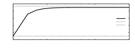 Figure 1
 Figure 0
 Figure 1
 Figure 10
 Figure 11
 Figure 12
 Figure 13
 Figure 14
 Figure 15
 Figure 16
 Figure 17
 Figure 18
 Figure 19
 Figure 2
 Figure 20
 Figure 21
 Figure 22
 Figure 23
 Figure 24
 Figure 25
 Figure 26
 Figure 27
 Figure 28
 Figure 29
 Figure 3
 Figure 30
 Figure 31
 Figure 32
 Figure 33
 Figure 34
 Figure 35
 Figure 36
 Figure 37
 Figure 38
 Figure 39
 Figure 4
 Figure 40
 Figure 41
 Figure 42
 Figure 43
| 0 | ||||||
|---|---|---|---|---|---|---|
Peer Reviews
No public reviews on file for this paper yet. If you reviewed it on a platform where reviews are public (OpenReview, ICLR, NeurIPS, ICML), you can paste yours below so the community can read it here.
Videos
No videos yet. Explain this paper in a talk, walkthrough, or lecture? Add one.
Factorized Runge–Kutta–Chebyshev Methods
Stephen O’Sullivan
School of Mathematical Sciences, Dublin Institute of Technology, Kevin Street, Dublin 8, Ireland
Abstract.
The second-order extended stability Factorized Runge–Kutta–Chebyshev (FRKC2) class of explicit schemes for the integration of large systems of PDEs with diffusive terms is presented. FRKC2 schemes are straightforward to implement through ordered sequences of forward Euler steps with complex stepsizes, and easily parallelised for large scale problems on distributed architectures. Preserving 7 digits for accuracy at 16 digit precision, the schemes are theoretically capable of maintaining internal stability at acceleration factors in excess of 6000 with respect to standard explicit Runge-Kutta methods. The stability domains have approximately the same extents as those of RKC schemes, and are a third longer than those of RKL2 schemes. Extension of FRKC methods to fourth-order, by both complex splitting and Butcher composition techniques, is discussed.
A publicly available implementation of the FRKC2 class of schemes may be obtained from maths.dit.ie/frkc
1. Introduction
Factorized Runge–Kutta–Chebyshev (FRKC) methods are well suited to the numerical integration of problems where diffusion limits the efficiency of standard explicit techniques. In general, such systems of PDEs may be presented as semi-discrete ordinary differential equations of the form
[TABLE]
Here, the associated Jacobian is assumed to have negative eigenvalues lying close to the real axis, a good approximation for many systems of interest in astrophysical contexts.
The main use of extended stability Runge–Kutta (ESRK) methods is to fill the gap between unconditionally stable but operationally complex implicit methods, and simply implemented explicit schemes which suffer from stability constraints for stiff problems. ESRK methods are particularly useful for problems involving diffusion, where the work required by standard explicit techniques goes as the inverse square of the mesh spacing, while for extended stability methods it goes as the inverse mesh spacing. ESRK explicit schemes may be broadly divided into factorized and recursive types.
Factorized ESRK methods are particularly straightforward to implement at second-order, consisting solely of forward Euler steps. At orders above two, splitting methods or, alternatively, additional finishing stages are required for nonlinear problems. First considered by [23, 9, 8], factorized ESRK methods fell out of common usage for some time, until revived in 1996 as SuperTimeStepping [4] at first-order, and later extended to second-order applications in astrophysical simulations by means of Richardson extrapolation [21, 22]. DUMKA methods exist at third- and fourth-order [16].
The perennial problem with the factorized formalism has been that, when a very large number of stages is used, the internal amplification factors can easily drown numerical precision. Factorized methods have, as a result, largely taken a back seat to recursive methods which manage internal stability by mapping the three-term recurrence relations for orthogonal polynomials to the stability polynomials [25]. Recursive methods have been developed up to fourth-order [27, 24, 3, 2, 15, 17, 18].
In the following, a formulation of factorized methods is presented which has high internal stability, and is more straightforward to implement than recursive methods, and demonstrates comparable efficiency.
2. FRKC stability polynomials
Stability polynomials form the backbone of ESRK numerical schemes and encapsulate the linear stability properties. Linearising a system of semi-discrete ODEs
[TABLE]
the FRKC stability polynomial [20] is obtained by seeking a polynomial of degree which yields a forward Euler scheme of order for linear problems through its roots via
[TABLE]
The -th stability polynomial of order , with , determined via , must match the first terms in the Taylor expansion of the evolution operator
[TABLE]
Equivalently, the linear order conditions may be expressed as constraints on the derivatives of the stability polynomial evaluated at zero:
[TABLE]
In addition, stability requires that the polynomial is bounded according to
[TABLE]
The objective is to determine a closed form for the polynomial such that the extent of the stability domain along the negative real axis is as great as possible.
It is shown in [20] that the FRKC stability polynomial of rank , and degree , is a sum of Chebyshev polynomials of the first kind given by
[TABLE]
where is the Chebyshev polynomial of the first kind of degree , and the coefficients are determined through the linear order conditions given by Equation 5. The resultant scheme follows immediately from the roots of the polynomial, , with coefficients given by
[TABLE]
The dependency of on is presented in Figure 1 at second-order (). While the optimal value for is [26], where is the conventional second order Runge–Kutta stability limit, values of 0.330, 0.333, and 0.25 are obtained for FRKC2, RKC [25], and RKL2 [18] respectively.
2.1. Damping
Along the real axis on the interior of the stability domain of the stability polynomial, there are points which are marginally stable, as shown in Figure 2. This is remedied by introducing the damping parameter via
[TABLE]
and again enforcing the order conditions given by Equation 5 via Newton-Raphson iteration over the parameters , which consist of distinct values, each repeated times. As a result, the marginally stable maxima in along the real axis are scaled by at the expense of reducing the extent of the stability domain along the real axis by approximately .
The damping process may also be used to make the scheme applicable to problems with small hyperbolic components, with Péclet numbers Pe\,\raisebox{-1.72218pt}{\stackrel{{\scriptstyle<}}{{\scriptstyle\sim}}}\,10. For the case , illustrated in Figure 2, there is a 25% loss in the extent of the stability domain observed.
2.2. Internal stability
Internal instability may be caused when the product of any of the possible sub-sequences of steps act to generate large values which drown out numerical precision. Following the idea of Lebedev [14, 13], but with a more effective approach, the timesteps are ordered to approximately minimise , where
[TABLE]
is the maximum over the internal amplification factors defined by
[TABLE]
While the optimal value of is approximately , for the purposes of constructing a stabilization algorithm, a practical upper bound of is chosen. In order to maintain this bound, the estimated maximum amplification factor is held to a minimum while runs from 1 to , where
[TABLE]
The amplification factors are defined by , where are uniformly distributed values over the reduced range , with . Initially, , however, in a limited number of cases, the process is repeated with incremented until the required bound is satisfied. In this work, the mean value of for the second-order schemes was found to be 1.5. Figure 3 shows the realised values of obtained via the stabilization algorithm for second-order schemes. Preserving 7 digits for accuracy, a scheme consisting of stages is therefore theoretically viable in a numerical integration carried out to 16 digit precision.
2.3. Convex Monotone Property
The convex monotone property (CMP) is of relevance to problems with spatially varying diffusion coefficients [18]. Figure 4 shows solutions obtained for a problem considered in [18] describing two materials placed into contact with differing temperatures and diffusion coefficients. For Chebyshev polynomial-based schemes such as RKC and FRKC2, noise in the solutions associated with failure to meet the CMP is evident if the schemes are forced to take steps with a uniform number of stages. Figures 4(a) and 4(b) illustrate this for the cases and respectively. The RKL2 scheme maintains the CMP naturally with the result that the solution is smooth (Figure 4(c)). As shown in Figure 4(d), for FRKC2 with an identical number of function evaluations as used for Figure 4(b), but with an error-control procedure (discussed further in Section 3), the noise is also absent.
3. FRKC2 schemes
A system is assumed such that the associated Jacobian has an eigenvalue of maximum magnitude . Then, given a numerical solution at some time index , stages (for ) are evaluated such that and a second-order accurate solution is obtained a time later. The intermediate stages of the scheme are determined via the Euler steps
[TABLE]
Error control is straightforward since a first-order solution is available at no additional cost in function evaluations. This first-order solution is obtained by considering only the real parts of and . Setting ,
[TABLE]
The error, scaled to a specified tolerance , is estimated using
[TABLE]
If , the step is rejected and retried with scaled by . Otherwise, a predictive controller is used to determine the subsequent timestep calibrated to the required tolerance via
[TABLE]
using values of and from previous timesteps. is a safety factor chosen with a value 0.8 here. The reader is referred to [11] for further details of error control procedures.
3.1. FRKC2 public code
A freely available C implementation of the second-order FRKC2 schemes may be accessed at maths.dit.ie/frkc. The files frkc2core.c and frkc2user.c provide the code for internal calculations required by the FRKC2 scheme and the code specific to the particular problem respectively. For a given value of , up to 257, the extent of the stability domain along the real axis, , and the maximum realised internal amplification factor (see also Figure 3) are given on line of frkc2arks.dat. The real and imaginary parts of are recorded on lines and respectively.
The default problem provided in frkc2user.c is a two-species reaction diffusion Brusselator
[TABLE]
which possesses a spectral radius of approximately for a mesh. The initial state is a perturbation of the equilibrium solution [19]which is given by , . Figure 5 shows the number of steps required to attain a given error in the solution for FRKC2, ROCK2 [1], and RKC. It is evident that, for a given precision, there is little difference in the number of steps required by FRKC2 and ROCK2. At higher degrees of acceleration (fewer steps), the difference between the three schemes is negligible.
4. FRKC4 scheme
4.1. Complex splitting
Above second-order, nonlinear order conditions are present which require additional consideration. One approach, given a semi-linear parabolic (reaction-diffusion) equation of the form , is to split the nonlinear part , which is typically easily integrated, from the linear diffusion terms . For orders above two, this requires complex timesteps [6, 5] and may be prescribed in the form
[TABLE]
Figure 6 shows the split FRKC4s scheme is competitive with ROCK4 [2]. However, in support of the splitting approach, it may be noted that ROCK4 suffers significantly from internal stability issues arising from the finishing stages required for the nonlinear order conditions (discussed further in Section 4.2) which effectively limits the scheme to about 150 stages.
4.2. Butcher composition
An alternative to complex splitting is Butcher composition. At fourth-order, as illustrated in Table 1, forward Euler steps are adopted from the FRKC stability polynomial with as the scheme , and appropriate finishing stages for the scheme are subsequently derived.
According to a theorem of Hairer & Wanner [10], given the B-series , , the composite scheme is determined via
[TABLE]
where rooted trees are used to represent derivatives in Taylor series. The first summation in Equation 19 is over all different labelings of , is the subtree formed by the first indices, and is the difference set of subtrees formed by the remaining indices. The eight order conditions at fourth order are then given by
[TABLE]
Hence, for given scheme , imposing the required order conditions on yields equations for , which are in turn easily solved for . The reader is referred to [10] for further details.
Figure 6 shows a comparison of the FRKC4 scheme based on composition methods with other schemes. The reference solution is provided by a fifth-order implicit preconditioned BDF solver from the CVODE numerical package [7]. The number of steps required for a given precision is comparable for ROCK4 and FRKC4 and somewhat greater than the split FRKC4s scheme. This difference may be ascribed to a loss of precision due to the accumulation of errors over the finishing stages [12].
5. Conclusions
FRKC extended stability Runge–Kutta (ESRK) schemes are shown to well-suited to the integration of large-scale problems governed by systems of PDEs where the explicit timescale is constrained by diffusion. An implementation of the FRKC2 second-order schemes, publicly available at maths.dit.ie/frkc, is presented. The fourth-order FRKC4 schemes are also presented with nonlinear order conditions addressed via both splitting and composition methods. These schemes are shown to be competitive with alternative ESRK methods.
5.1. Acknowledgments
I am grateful to organisers of Astronum2016 for the invitation to present this work in Monterey and to an anonymous referee for helpful comments.
6. References
The reference list from the paper itself. Each links out to its DOI / PubMed record.
- 1[1] Assyr Abdulle. Chebyshev methods based on orthogonal polynomials . Ph D thesis, 2001.
- 2[2] Assyr Abdulle. Fourth order Chebyshev methods with recurrence relation. SIAM Journal on Scientific Computing , 23(6):2041–2054, 2002.
- 3[3] Assyr Abdulle and Alexei A Medovikov. Second order Chebyshev methods based on orthogonal polynomials. Numerische Mathematik , 90(1):1–18, 2001.
- 4[4] V. Alexiades, G. Amiez, and P.A. Gremaud. Super-time-stepping acceleration of explicit schemes for parabolic problems. Communications in numerical methods in engineering , 12(1):31–42, 1996.
- 5[5] Sergio Blanes, Fernando Casas, Philippe Chartier, and Ander Murua. Optimized high-order splitting methods for some classes of parabolic equations. Mathematics of Computation , 82(283):1559–1576, 2013.
- 6[6] F. Castella, P. Chartier, S. Descombes, and G. Vilmart. Splitting methods with complex times for parabolic equations. BIT Numerical Mathematics , 49:487–508, 2009.
- 7[7] Scott D Cohen and Alan C Hindmarsh. CVODE, a stiff/nonstiff ODE solver in C. Computers in physics , 10(2):138–143, 1996.
- 8[8] W Gentzsch and A Schluter. On one-step methods with cyclic stepsize changes for solving parabolic differential equations. Z. Angew. Math. Mech , 58:T 415–T 416, 1978.