Noise sensitivity of functionals of fractional Brownian motion driven stochastic differential equations: Results and perspectives
Alexandre Richard, Denis Talay

TL;DR
This paper investigates how the probability distributions of functionals of solutions to fractional Brownian motion driven stochastic differential equations change as the Hurst parameter approaches 1/2, extending Gaussian density estimates uniformly.
Contribution
It introduces a novel sensitivity analysis method for SDEs driven by fractional Brownian motion, focusing on the limit as H approaches 1/2, with uniform Gaussian estimates.
Findings
Extended Gaussian density estimates uniformly in time and Hurst parameter.
Analyzed the sensitivity of first passage times as H approaches 1/2.
Provided new perspectives on fractional Brownian motion driven SDEs.
Abstract
We present an innovating sensitivity analysis for stochastic differential equations: We study the sensitivity, when the Hurst parameter~ of the driving fractional Brownian motion tends to the pure Brownian value, of probability distributions of smooth functionals of the trajectories of the solutions and of the Laplace transform of the first passage time of at a given threshold. Our technique requires to extend already known Gaussian estimates on the density of to estimates with constants which are uniform w.r.t. in in the whole half-line and when tends to~.
Click any figure to enlarge with its caption.
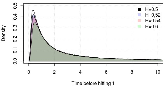 Figure 1
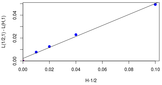 Figure 2
| – | – | – | – | |||||
| Error (%) | Error (%) | ||||
|---|---|---|---|---|---|
| Error (%) | Error (%) | ||||
|---|---|---|---|---|---|
Peer Reviews
No public reviews on file for this paper yet. If you reviewed it on a platform where reviews are public (OpenReview, ICLR, NeurIPS, ICML), you can paste yours below so the community can read it here.
Videos
No videos yet. Explain this paper in a talk, walkthrough, or lecture? Add one.
Taxonomy
TopicsStochastic processes and financial applications · Financial Risk and Volatility Modeling · Complex Systems and Time Series Analysis
Noise sensitivity of functionals of fractional Brownian motion
driven stochastic differential equations: Results and perspectives
Alexandre Richard
CMAP, École Polytechnique, Route de Saclay, 91128 Palaiseau, France
Denis Talay
INRIA Sophia-Antipolis, 2004 route des Lucioles, F-06902 Sophia-Antipolis, France
(March 3, 2024)
Abstract
We present an innovating sensitivity analysis for stochastic differential equations: We study the sensitivity, when the Hurst parameter of the driving fractional Brownian motion tends to the pure Brownian value, of probability distributions of smooth functionals of the trajectories of the solutions and of the Laplace transform of the first passage time of at a given threshold. Our technique requires to extend already known Gaussian estimates on the density of to estimates with constants which are uniform w.r.t. in in the whole half-line and when tends to .
Key words: Fractional Brownian motion, Malliavin calculus, first hitting time.
1 Introduction
Recent statistical studies show memory effects in biological, financial, physical data: see e.g. [18] for a statistical evidence in climatology and [6] for a financial model and citations therein for evidence in finance. For such data the Markov structure of Lévy driven stochastic differential equations makes such models questionable. It seems worth proposing new models driven by noises with long-range memory such as fractional Brownian motions.
In practice the accurate estimation of the Hurst parameter of the noise is difficult (see e.g. [4]) and therefore one needs to develop sensitivity analysis w.r.t. of probability distributions of smooth and non smooth functionals of the solutions to stochastic differential equations. Similar ideas were developed in [11] for symmetric integrals of the fractional Brownian motion.
Here we review and illustrate by numerical experiments our theoretical results obtained in [17] for two extreme situations in terms of Malliavin regularity: on the one hand, expectations of smooth functions of the solution at a fixed time; on the other hand, Laplace transforms of first passage times at prescribed thresholds. Our motivation to consider first passage times comes from their many use in various applications: default risk in mathematical finance or spike trains in neuroscience (spike trains are sequences of times at which the membrane potential of neurons reach limit thresholds and then are reset to a resting value, are essential to describe the neuronal activity), stochastic numerics (see e.g. [3, Sec.3]) and physics (see e.g. [13]). Long-range dependence leads to analytical and numerical difficulties: see e.g. [10].
Our theoretical estimates and numerical results tend to show that the Markov Brownian model is a good proxy model as long as the Hurst parameter remains close to . This robustness property, even for probability distributions of singular functionals (in the sense of Malliavin calculus) of the paths such as first hitting times, is an important information for modeling and simulation purposes: when statistical or calibration procedures lead to estimated values of close to , then it is reasonable to work with Brownian SDEs, which allows to analyze the model by means of PDE techniques and stochastic calculus for semimartingales, and to simulate it by means of standard stochastic simulation methods.
Our main results
The fractional Brownian motion with Hurst parameter is the centred Gaussian process with covariance
[TABLE]
Given , we consider the process solution to the following stochastic differential equation driven by :
[TABLE]
where the last integral is a pathwise Stieltjes integral in the sense of [19]. For the process solves the following SDE in the classical Stratonovich sense:
[TABLE]
Below we use the following set of hypotheses:
- (H1)
There exists such that ; 2. (H2)
; 3. (H3)
The function satisfies a strong ellipticity condition: such that .
Our first theorem is elementary. It describes the sensitivity w.r.t. around the critical Brownian parameter of time marginal probability distributions of .
Theorem 1.1**.**
Let , and let and be as before. Suppose that and satisfy (H1) and (H3), and is bounded and Hölder continuous of order for some . Then, for any there exists such that
[TABLE]
Our next theorem concerns the first passage time at threshold 1 of issued from : . The probability distribution of the first passage time of a fractional Brownian motion is not explictly known. [14] obtained the asymptotic behaviour of its tail distribution function and [7] obtained an upper bound on the Laplace transform of . The recent work of [8] proposes an asymptotic expansion (in terms of ) of the density of formally obtained by perturbation analysis techniques.
Theorem 1.2**.**
Suppose that and satisfy Hypotheses (H2) and (H3) and let . There exist constants , (both depending on and only), and such that: for all and , there exists such that
[TABLE]
where . In the pure fBm case (where and ) the result holds with and .
To prove the preceding theorem we need accurate estimates on the density of with constants which are uniform w.r.t. small and long times and w.r.t. in . Our next theorem improves estimates in [2, 5]. Our contributions consists in getting constants which are uniform w.r.t. in the whole half-line and when tends to .
Theorem 1.3**.**
Assume that and satisfy the conditions (H2) and (H3). Then for every , the density of satisfies: there exists such that, for all and ,
[TABLE]
Note that Theorems 1.1, 1.2 and 1.3 are proved in [17], including extensions to . We do not address the proof of Theorem 1.3 here.
We sketch the proofs of Theorems 1.1 and 1.2 in Section 2. In Section 3 we consider a case which was not tackled in [17], that is, the case . Finally, in Section 4 we show numerical experiment results which illustrate Theorem 1.2 and suggest that the rate is sub-optimal.
2 Sketch of the proofs
2.1 Reminders on Malliavin calculus
We denote by and the classical derivative and Skorokhod operators of Malliavin calculus w.r.t. Brownian motion on the time interval (see e.g. [15]). In the fractional Brownian motion framework the Malliavin derivative is defined as an operator on the smooth random variables with values in the Hilbert space defined as the completion of the space of step functions on with the following scalar product:
[TABLE]
where .
The domain of in () is denoted by and is the closure of the space of smooth random variables with respect to the norm:
[TABLE]
Equivalently, and are defined as and for (cf. [15, p.288]), where for any the operator is defined as follows: for any with suitable integrability properties,
[TABLE]
with
[TABLE]
We denote by the sup norm and the Hölder norm for functions on the interval . Under Assumption (H3), there exists a transformation called the Lamperti transform, such that is mapped to the solution of (1;H) with coefficients and . Since is one-to-one, we assume in the rest of this paper that is uniformly . See [17] for details on the Lamperti transform in this framework.
Let be the solution to (1;H). There exist modifications of the processes and such that for any it a.s. holds that
[TABLE]
These inequalities are simple consequences of the definition of , assumptions (H1) and (H3), and the equality: (see Section 3 in [17] for more details).
2.2 Sketch of the proof of Theorem 1.1
Proving Theorem 1.1 is easy. A first technique consists in using pathwise estimates on with and defined on the same probability space. A second technique, which we present here in order to introduce the reader to the method of proof for Theorem 1.2, consists in differentiating where
[TABLE]
which leads to
[TABLE]
As solves a parabolic PDE driven by the generator of and as the Skorokhod integral has zero mean we get
[TABLE]
It then remains to use the estimates (2.1).
2.3 Sketch of the proof of Theorem 1.2
We now sketch the proof of Theorem 1.2. We will soon limit ourselves to the pure fBm case ( and ) in order to show the main ideas used in the proof and avoid too many technicalities. For now, our previous remark on the Lamperti transform implies that can be chosen uniformly equal to .
Our Laplace transforms sensititivity analysis is based on a PDE representation of first hitting time Laplace transforms in the case .
For it is well known that
[TABLE]
where the function is the classical solution with bounded continuous first and second derivatives to
[TABLE]
For any the process \mathbf{1}_{[0,t]}u_{\lambda}^{\prime}(B^{H}_{\scalebox{0.4}{\bullet}})\ e^{-\lambda{\scalebox{0.4}{\bullet}}} is in . One thus can apply Itô’s formula to (see [17, Section 2] and [15]). As satisfies (2.2), for any we get
[TABLE]
where the last term corresponds to the Itô term. Using and the ODE (2.2) satisfied by , we get
[TABLE]
where . Observe that the last term vanishes for close to , since is an approximation of the identity and converges to [math] as . This argument is made rigorous in [17].
We now limit ourselves to the pure fBm case ( and ) to make the rest of the computations more understandable, although the differences will be essentially technical. Given that now, , the previous equality becomes
[TABLE]
Evaluate the previous equation at , take expectations and let tend to infinity. For any it comes:
[TABLE]
Proposition 2.1**.**
Let be the function of defined by if and if . There exists a constant such that
[TABLE]
where is the function defined in Theorem 1.2.
Sketch of proof.
From Fubini’s theorem, we get
[TABLE]
The inequalities
[TABLE]
and
[TABLE]
lead to the desired result. ∎
Note that this proof adapts to diffusions, but that the density of is now needed, which is the purpose of Theorem 1.3.
Compared to the proof of Theorem 1.1, an important difficulty appears when estimating : as the optional stopping theorem does not hold for Skorokhod integrals of the fBm one has to carefully estimate expectations of stopped Skorokhod integrals and obtain estimates which decrease infinitely fast when goes to infinity. We obtained the following result.
Proposition 2.2**.**
[TABLE]
Proof.
Proposition 13 of [16] shows that
[TABLE]
Thus satisfies
[TABLE]
Define the field and the process by
[TABLE]
and
[TABLE]
For any real-valued function with one has
[TABLE]
Therefore
[TABLE]
Suppose for a while that we have proven: there exists such that for all and all , there exist constants such that
[TABLE]
We would then get:
[TABLE]
which is the desired result (2.5).
In order to estimate the left-hand side of Inequality (2.7) we aim to apply Garsia-Rodemich-Rumsey’s lemma (see below). However, it seems hard to get the desired estimate by estimating moments of increments of , in particular because is not smooth in the Malliavin sense. We thus proceed by localization and construct a continuous process which is smooth on the event and is close to 0 on the complementary event. To this end we introduce the following new notations.
For some small to be fixed set
[TABLE]
and
[TABLE]
where is a smooth function taking values in such that , and .
The crucial property of is the following: For all and , a.s. This is a consequence of the local property of ([15, p.47]). Therefore, for any ,
[TABLE]
Recall the Garsia-Rodemich-Rumsey lemma: if is a continuous process, then for and such that , one has
[TABLE]
provided the right-hand side in each line is finite. In order to apply (2.3), we thus need to estimate moments of . Note that Lemmas 2.3 and Lemmas 2.4 (below) both give bounds on the moments of in terms of a power of . Thus has a continuous modification, by Kolmogorov’s continuity criterion, and the GRR lemma will be applicable to .
We can easily obtain bounds on the norm in terms of . This observation leads us to notice that
[TABLE]
We then combine Lemmas 2.3 and 2.4 below to obtain: For every ,
[TABLE]
Choosing and we thus get
[TABLE]
from which Inequality (2.7) follows. ∎
It now remains to prove the above estimates on and : These estimates are provided by Lemmas 2.3 and 2.4 below whose proofs are very technical.
Lemma 2.3**.**
There exists such that: for all , for all and for all , there exist such that
[TABLE]
where the function is defined as in Theorem 1.2.
Lemma 2.4**.**
There exists such that: For all and , there exist such that
[TABLE]
3 Discussion on the fBm case with
We believe that Theorem 1.2 also holds true for . One of the main issues consists in getting accurate enough bounds on the right-hand side of Inequality (2.6).
For and () we have
[TABLE]
We here limit ourselves to examine the second summand on the r.h.s and we denote it by . The two other terms (corresponding to and ) are easier to study.
Compared to Subsection 2.3 we localize the Skorokhod integral in a slightly different manner by using instead of , where denotes the running supremum of the fBm up to time . Hence
[TABLE]
Set and
[TABLE]
Proceeding as from Eq.(2.8) to Eq.(2.3) we get for some and (chosen later):
[TABLE]
We then use the proposition 3.2.1 in [15] to bound :
[TABLE]
The Malliavin derivative of the supremum of the fBm is obtained for example in [7]. Denoting by the first time at which reaches on the interval we have . It follows that . Since , we are led to study the three following terms (for ):
- (i)
. 2. (ii)
3. (iii)
We do not know any accurate estimate on the joint law of either (S^{H}_{\scalebox{0.4}{\bullet}},B^{H}_{\scalebox{0.4}{\bullet}}) or (S^{H}_{\scalebox{0.4}{\bullet}},\vartheta_{\scalebox{0.4}{\bullet}}). We thus can only use the rough bounds for (ii) and for (iii). Then one is in a position to use the following refinement of Molchan’s asymptotic [14] obtained by Aurzada [1]: for some constant . However, when plugged into (3.2) and then into (3), these bounds lead us to an upper bound for which diverges when .
Hence the preceding rough bounds on (ii) and (iii) must be improved. In the Brownian motion case, the joint laws of and are known (see e.g. [12, p.96–102]). In particular, for the term (iii) leads to
[TABLE]
instead of the bound when one uses the previous rough method.
From numerical simulations and an incomplete mathematical analysis using arguments developed by [14] and [1] we believe that Inequality (3.3) remains true for . If so, the bound on would become
[TABLE]
which, in view of and , can now be bounded as .
4 Optimal rate of convergence in Theorem 1.2:
Comparison with numerical results
In this section, we numerically approximate the quantity , where is the first time a fractional Brownian motion started from [math] hits .
As already recalled this Laplace transform is explictely known in the Brownian case: , . Our simulations suggest that the convergence of towards is faster than what we were able to prove. We also show numerical experiments which concern the convergence of hitting time densities.
Although several numerical schemes permit to decrease the weak error when estimating , none seem to be available in the fractional Brownian motion case. We thus propose a heuristic extension of the bridge correction of Gobet [9] (valid in the Markov case) and compare this procedure to the standard Euler scheme.
Convergence of to \mathbb{E}\big{[}e^{-\lambda\tau_{\frac{1}{2}}}\big{]}.
Let us fix a time horizon and points on each trajectory. Let be the time step. Denote by the number of Monte-Carlo samples. For each , we simulate , from which we obtain . We then approximate as follows:
[TABLE]
The bias due to the time discretization implies .
In view of Theorem 1.2 we have
[TABLE]
with . We approximate by for several values of close to and then perform a linear regression analysis around . The slope of the regression line provides a hint on the optimal value of .
Notice that the global error results from the discretization error and the statistical error . The chosen number of simulations is such that , for some numerical constant .
The numerical results are presented in Table 1 for several values of and of the parameter . These results suggest that is linear w.r.t. . For each we thus perform a linear regression on these quantities (without the above transformation). The regression line is plotted in Fig. 1.
Our numerical results suggest that Theorem 1.2 is not optimal but the optimal convergence rate seems hard to get. An even more difficult result to obtain concerns the convergence rate of the density of the first hitting time of fBm to the density of the first hitting time of Brownian motion. We analyze it numerically: See Fig. 2.
Brownian bridge correction. We apply the following rule (which is only heuristic when ): at each time step, if the threshold has not yet been hit and if and , we sample a uniform random variable on and compare it to
[TABLE]
If then decide . Otherwise let the algorithm continue. We denote by the corresponding Laplace transform. This algorithm is an adaptation to a non-Markovian framework of the algorithm of [9], which is rigorously proven when . In particular is exactly the probability that a Brownian motion conditioned by its values at time and crosses in the time interval .
Table 2 shows the corresponding results for the simple estimator and the Brownian Bridge estimator with in the Brownian case (we kept ). Consistently with theoretical results, Table 2 shows that the estimator allows to substantially reduce the number of discretization steps (thus the computational time) to get a desired accuracy. The figure also shows a reasonable choice of which we actually keep when tackling the fractional Brownian motion case.
The exact value is unknown. Our reference value is the lower bound . The parameter used in Table 3 allows to conjecture that the Brownian bridge correction is useful even in the non-Markovian case. Although the approximation errors of the estimators and are similar when compared to , we recommend to use the latter because we have whereas .
Appendix: tables
The reference list from the paper itself. Each links out to its DOI / PubMed record.
- 1[1] F. Aurzada. On the one-sided exit problem for fractional Brownian motion. Electron. Commun. Probab. , 16 :392–404, 2011.
- 2[2] F. Baudoin, C. Ouyang and S. Tindel. Upper bounds for the density of solutions to stochastic differential equations driven by fractional Brownian motions. Ann. Inst. Henri Poincaré Probab. Stat. , 50 (1):111–135, 2014.
- 3[3] F. Bernardin, M. Bossy, C. Chauvin, J.-F. Jabir and A. Rousseau. Stochastic Lagrangian method for downscaling problems in meteorology. M 2AN Math. Model. Numer. Anal. , 44 (5):885–920, 2010.
- 4[4] C. Berzin, A. Latour and J.R. León. Inference on the Hurst Parameter and the Variance of Diffusions Driven by Fractional Brownian Motion . Springer, 2014.
- 5[5] M. Besalú, A. Kohatsu-Higa and S. Tindel. Gaussian type lower bounds for the density of solutions of SD Es driven by fractional Brownian motions. Ann. Probab. , 44 (1):399–443, 2016.
- 6[6] F. Comte, L. Coutin and É. Renault. Affine fractional stochastic volatility models. Ann. Finance , 8 :337–378, 2012.
- 7[7] L. Decreusefond and D. Nualart. Hitting times for Gaussian processes. Ann. Probab. , 36 (1):319–330, 2008.
- 8[8] M. Delorme and K. J. Wiese. Maximum of a fractional Brownian motion: analytic results from perturbation theory. Phys. Rev. Lett. , 115 :210601, Nov 2015.