Globally convergent Jacobi-type algorithms for simultaneous orthogonal symmetric tensor diagonalization
Jianze Li, Konstantin Usevich, Pierre Comon

TL;DR
This paper introduces and proves the global convergence of new Jacobi-type algorithms for the simultaneous orthogonal diagonalization of symmetric tensors and matrices, advancing tensor decomposition methods.
Contribution
It extends Jacobi algorithms to symmetric tensors and establishes their global convergence, including a new algorithm for smooth functions.
Findings
Proved global convergence for existing Jacobi algorithm on matrices and third-order tensors.
Developed a new Jacobi-based algorithm with proven convergence for smooth functions.
Enhanced tensor diagonalization techniques for symmetric tensors.
Abstract
In this paper, we consider a family of Jacobi-type algorithms for simultaneous orthogonal diagonalization problem of symmetric tensors. For the Jacobi-based algorithm of [SIAM J. Matrix Anal. Appl., 2(34):651--672, 2013], we prove its global convergence for simultaneous orthogonal diagonalization of symmetric matrices and 3rd-order tensors. We also propose a new Jacobi-based algorithm in the general setting and prove its global convergence for sufficiently smooth functions.
Click any figure to enlarge with its caption.
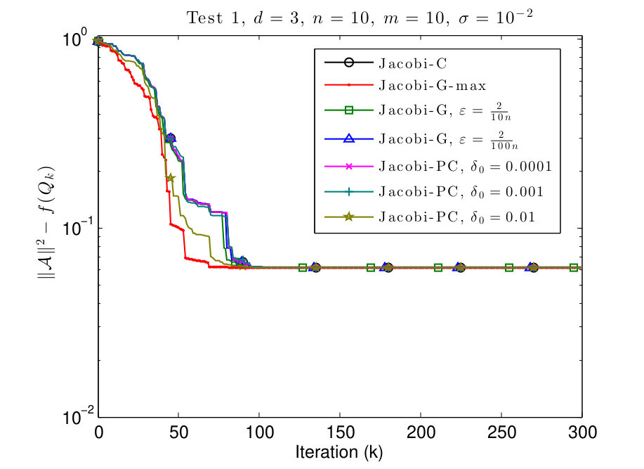 Figure 1
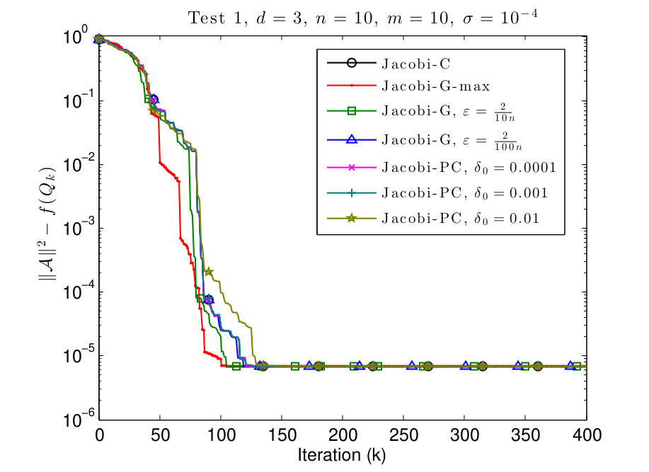 Figure 2
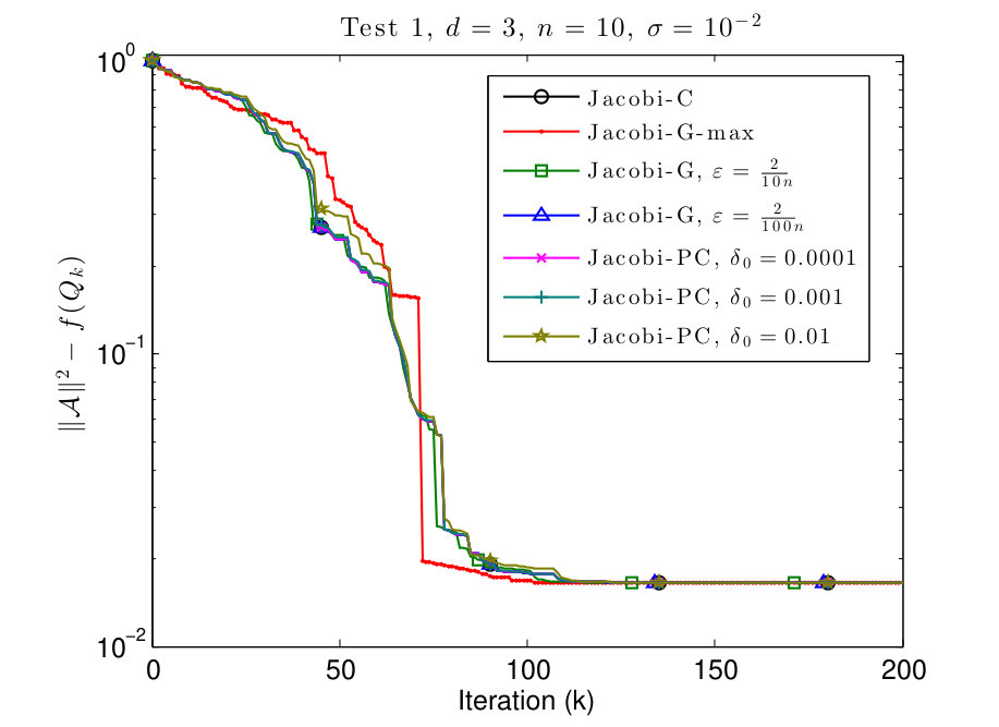 Figure 3
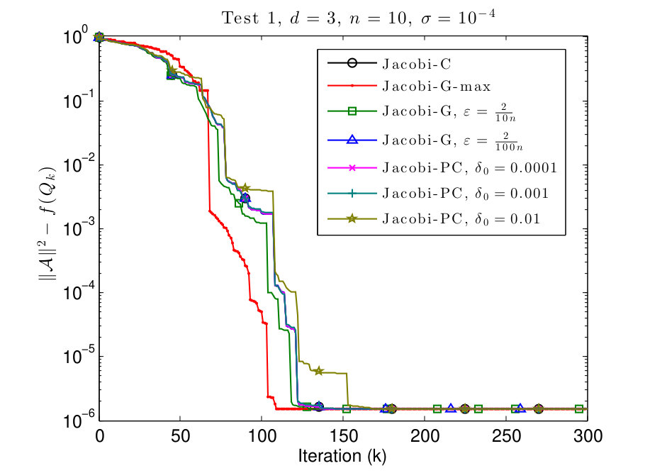 Figure 4
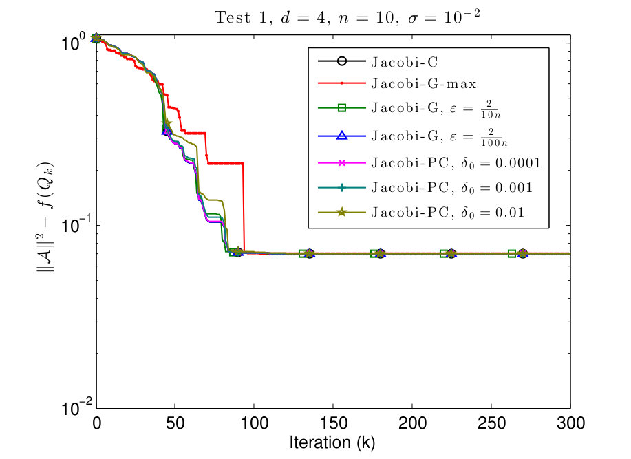 Figure 5
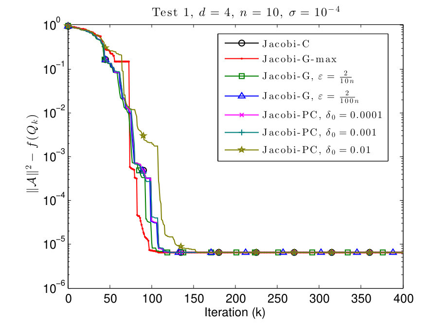 Figure 6
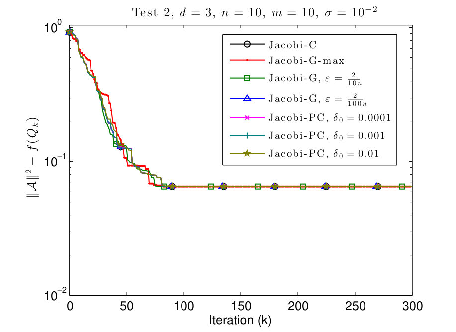 Figure 7
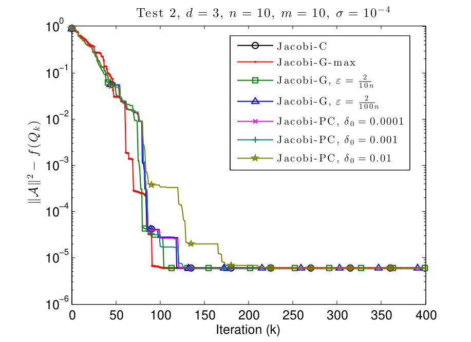 Figure 8
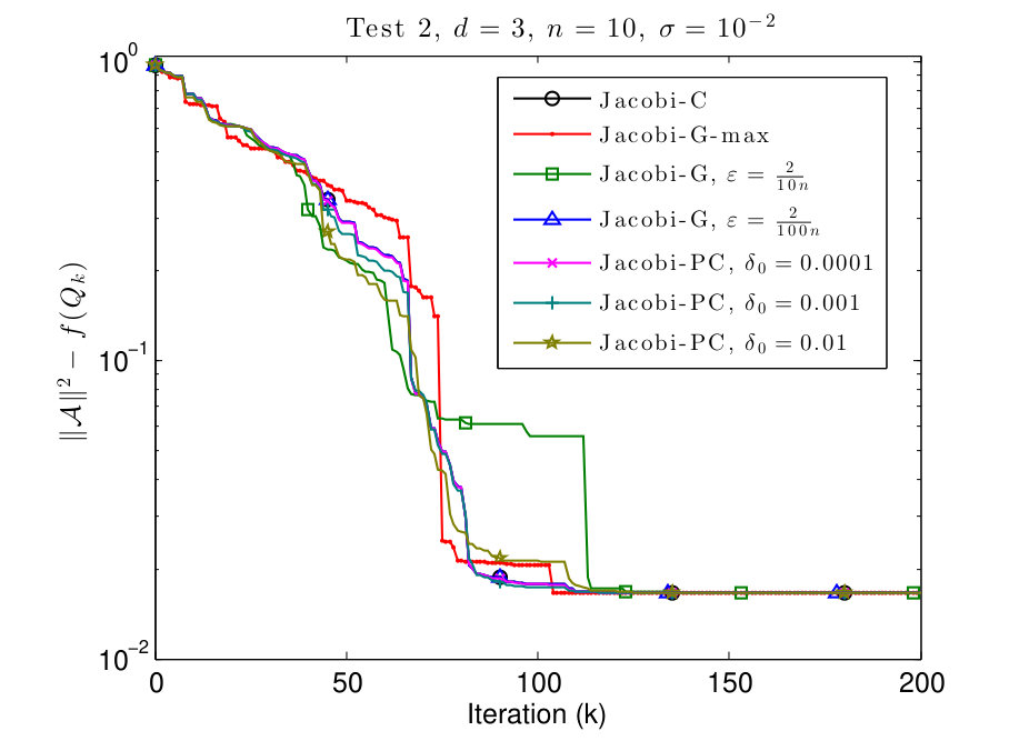 Figure 9
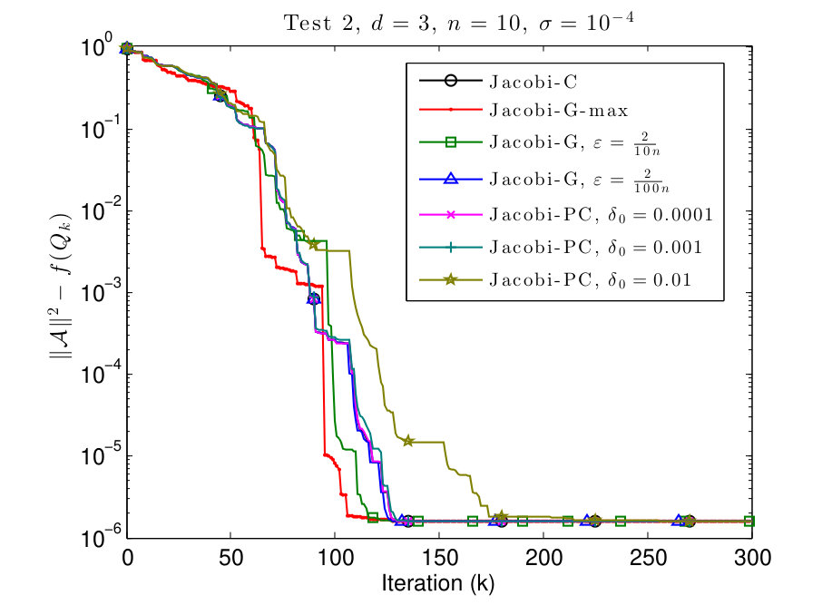 Figure 10
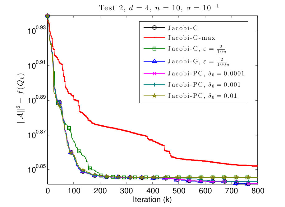 Figure 11
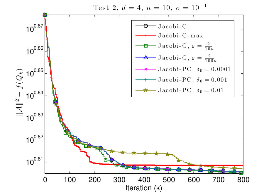 Figure 12
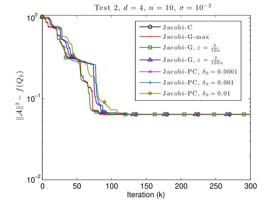 Figure 13
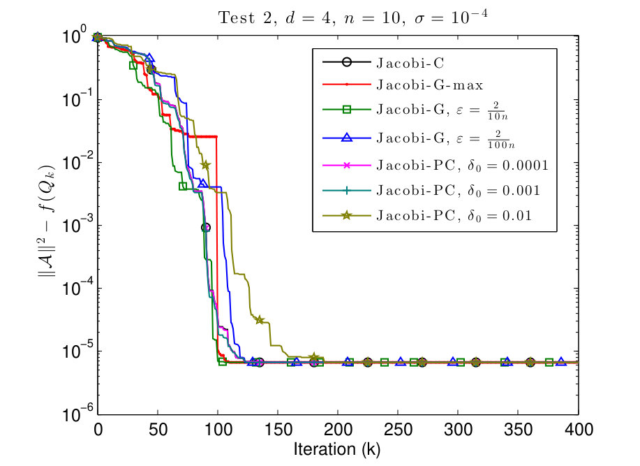 Figure 14
Peer Reviews
No public reviews on file for this paper yet. If you reviewed it on a platform where reviews are public (OpenReview, ICLR, NeurIPS, ICML), you can paste yours below so the community can read it here.
Videos
No videos yet. Explain this paper in a talk, walkthrough, or lecture? Add one.
Taxonomy
TopicsTensor decomposition and applications · Matrix Theory and Algorithms · Sparse and Compressive Sensing Techniques
\headers
Globally convergent Jacobi-type algorithmsJ. Li, K. Usevich, and P. Comon
Globally convergent Jacobi-type algorithms
for simultaneous orthogonal
symmetric tensor diagonalization††thanks: Submitted to the editors DATE. \fundingThis work was supported by the ERC project “DECODA” no.320594, in the frame of the European program FP7/2007-2013. The first author was partially supported by the National Natural Science Foundation of China (No.11601371).
Jianze Li School of Mathematics, Tianjin University, Tianjin 300072, China (). [email protected]
Konstantin Usevich GIPSA-Lab, CNRS and Univ. Grenoble Alpes, France (). [email protected]
Pierre Comon33footnotemark: 3
Abstract
In this paper, we consider a family of Jacobi-type algorithms for simultaneous orthogonal diagonalization problem of symmetric tensors. For the Jacobi-based algorithm of [SIAM J. Matrix Anal. Appl., 2(34):651–672, 2013], we prove its global convergence for simultaneous orthogonal diagonalization of symmetric matrices and 3rd-order tensors. We also propose a new Jacobi-based algorithm in the general setting and prove its global convergence for sufficiently smooth functions.
keywords:
orthogonal tensor diagonalization, Jacobi rotation, global convergence, Łojasiewicz gradient inequality, proximal algorithm
{AMS}
15A69, 49M30, 65F99, 90C30
1 Introduction
Higher-order tensor decompositions have attracted a lot of attention in the last two decades because of the applications in various disciplines, including signal processing, numerical linear algebra and data analysis [5, 9, 20]. The most popular decompositions include the Canonical Polyadic and Tucker decompositions, where additional constraints are often imposed, such as symmetry [10], nonnegativity [22] or orthogonality [19].
An important class of tensor approximation problems is approximation with orthogonality constraints. In particular, the orthogonal symmetric tensor diagonalization problem for 3rd and 4th-order cumulant tensors is in the core of Independent Component Analysis [6, 7, 8], and is a popular way to solve blind source separation problems in signal processing [11]. In the same context, simultaneous orthogonal matrix diagonalization [4] is widely used; simultaneous orthogonal tensor diagonalization for slices of 4th-order cumulants is also used to solve source separation problems [16].
Main notations
Let denote the space of th-order tensors. In the paper, the tensors are typeset with a bold calligraphic font (e.g, , ), and matrices are in bold (e.g, , ); the elements of tensors or matrices are typeset as (or sometimes ) or respectively.
For a tensor and a matrix , their -mode product [20, subsection 2.5] is the tensor defined as
[TABLE]
A tensor is called symmetric if its entries do not change under any permutation of indices; its diagonal is, by definition, the vector
[TABLE]
We will always denote by the Frobenius norm of a tensor or a matrix, or the Euclidean norm of a vector. Finally, let denote the orthogonal group, that is, the set of orthogonal matrices. Let denote the special orthogonal group, the set of orthogonal matrices with determinant .
Problem statement
In this paper, we consider the following simultaneous orthogonal symmetric tensor diagonalization problem. Let be a set of symmetric tensors. We wish to maximize
[TABLE]
where for . Problem Eq. 1 has the following well-known problems as special cases:
- •
orthogonal tensor diagonalization problem if and ;
- •
simultaneous orthogonal matrix diagonalization problem if and .
Several algorithms have been proposed in the literature to solve special cases of problem Eq. 1. The first were the Jacobi CoM (Contrast Maximization) algorithm for orthogonal diagonalization of 3rd and 4th-order symmetric tensors [6, 7, 8] and the JADE (Joint Approximate Diagonalization of Eigenmatrices) algorithm for simultaneous orthogonal matrix diagonalization [4]. An algorithm for simultaneous orthogonal 3rd-order tensor diagonalization was proposed in [14]. These Jacobi-type algorithms have been very widely used in applications [11], and have the advantage that Jacobi rotations can be computed by rooting low-order polynomials. Nevertheless, up to our knowledge, the convergence of these methods was not proved, although it was often observed in practice [8, 13].
Contribution
In this paper, we consider several Jacobi-type algorithms to solve problem Eq. 1, and study their global convergence properties. By global convergence, we mean that, for any starting point, the whole sequence of iterations produced by the algorithm always converges to a limit point111This was also called single-point convergence in [26].. Note that the global convergence does not guarantee convergence to a global maximum, since the cost function is multimodal.
First, we consider the Jacobi-based algorithm proposed in [17] for best low multilinear rank approximation of 3rd-order symmetric tensors. The algorithm uses a gradient-based order of Jacobi rotations, hence we call this algorithm Jacobi-G in our paper. For the Jacobi-G algorithm the convergence of subsequences of iterations to stationary points was established in [17]. We prove that, for problem Eq. 1, Jacobi-G algorithm converges globally and the limit point is always a stationary point in the cases . The proof is based on a variant Łojasiewicz theorem developed in [25] for analytic submanifolds of Euclidean space.
Second, we propose a new Jacobi-based algorithm inspired by proximal methods [24], which is called the Jacobi-PC algorithm in this paper. We show that Jacobi-PC algorithm always converges globally to a stationary point in the general setting. In particular, for cases of problem Eq. 1, Jacobi-PC algorithm allows for a simple algebraic solution to find the optimal Jacobi rotation, as in the Jacobi CoM algorithm [6, 7, 8]. In addition, this algorithm does not need the order of Jacobi rotations introduced in Jacobi-G algorithm. Finally, the global convergence of Jacobi-PC algorithm is proved for sufficiently smooth functions. Therefore, these results may be applied to other tensor approximation problems (e.g., nonsymmetric orthogonal diagonalization [23],or Tucker approximation of symmetric [17] or antisymmetric [3] tensors).
Organization
The paper is organized as follows. In Sections 2 to 4, we present some more or less known results or easy extensions. In Sections 5 to 7, we show our main results of this paper. In Section 2, we introduce the abstract optimization problem on and the general Jacobi algorithm to solve this abstract problem. In Section 3, we recall the Jacobi-G algorithm proposed in [17] and its local convergence properties in the general setting. In Section 4, we list some properties that are specific to orthogonal tensor diagonalization problem. In Section 5, we prove the global convergence of Jacobi-G algorithms for simultaneous orthogonal diagonalization of matrices and 3rd-rder tensors. In Section 6, we propose the Jacobi-PC algorithm and prove its global convergence. We derive formulas for optimal Jacobi rotations in the case of 3rd and 4th-order tensors. In Section 7, we provide some numerical experiments.
2 Problem statement and Jacobi rotations
2.1 Abstract optimization problem
Let be a function. The abstract optimization problem is to find such that
[TABLE]
Example 1**.**
Problem Eq. 1 in Section 1 is a special case of problem Eq. 2. Because for any , problem Eq. 1 is equivalent to find
[TABLE]
*where is the vector of elements in except diagonal elements. *
Example 2**.**
In [17], the best low multilinear rank approximation problem for 3rd order symmetric tensors was formulated as a special case of problem Eq. 2. In fact, based on [15, Theorem 4.1], the cost function has the form
[TABLE]
*where and . *
Example 3**.**
*Under some assumptions, it was shown that the orthogonal tensor diagonalization problem could be solved in the sense of maximization of the trace of a tensor [12], and is also a special case of problem Eq. 2. *
2.2 Givens rotations and the general Jacobi algorithm
Let be an angle and be a pair of indices with . We denote the Givens rotation matrix by
[TABLE]
i.e., the matrix defined by
[TABLE]
for . We summarize the general Jacobi algorithm in Algorithm 1.
Note that in Algorithm 1 (and all the following algorithms, unless mentioned explicitly) we do not specify a stopping criterion, since our goal is to analyse the whole sequence of iterations produced by the algorithm. The stopping criterion applies only to software implementation of algorithms.
Algorithm 1 performs the sequence of iterations by multiplicative updates:
[TABLE]
where each is an elementary rotation. The advantage of this Jacobi-type algorithm is that each update is a one-dimensional optimization problem, which can be solved efficiently.
Remark 2.1**.**
Note that the choice of pair in every iteration is not specified in Algorithm 1. One of the most natural rules is in cyclic fashion as follows.
[TABLE]
*We call the Jacobi algorithm with this cyclic-by-row rule the Jacobi-C algorithm. *
In Jacobi-C algorithm, the choice of pairs is periodic with the period . Each set of iterations is called a sweep. The pair selection rule Eq. 6 was used in the Jacobi CoM algorithm [6, 7, 8] and JADE algorithm [4].
Remark 2.2**.**
*If several equivalent maximizers are present in Eq. 4, also in all the following algorithms, we choose the one with the angle of smaller magnitude. *
3 Jacobi-G algorithm
In this section, we recall the Jacobi-based algorithm in [17] and its properties. For simplicity, this algorithm is called the Jacobi-G (gradient-based Jacobi-type) algorithm in our paper.
3.1 Technical definitions
Define the matrix
[TABLE]
and introduce the notation
[TABLE]
for . Next, for a differentiable function , we define the projected gradient [17, Lemmma 5.1] as
[TABLE]
where
[TABLE]
and is the Euclidean gradient of as a function of the matrix argument. The projected gradient is exactly the Riemannian gradient if is viewed as an embedded submanifold of [2].
3.2 Jacobi-G algorithm
In [17], a modification of Algorithm 1 was proposed, that choose a pair at each iteration that satisfies
[TABLE]
where is a small positive constant.
Note that, as shown in [17, Proof of Lemma 5.3] the left hand side of Eq. 9 can be also written in terms of the function :
[TABLE]
The following lemma (an easy generalisation of [17, Lemma 5.2]) shows that it is always possible to choose such a pair .
Lemma 3.1**.**
*For any differentiable function , and , it is always possible to find , with , such that (9) holds. *
Proof 3.2**.**
First of all, thanks to the representation (7), rotation invariance of the Euclidean norm and being skew-symmetric, we have that the condition (9) is equivalent to
[TABLE]
Now we choose the pair that maximizes the left-hand side of (11)
[TABLE]
Since is skew-symmetric, we can choose such a pair with . Finally, by the well known inequality between matrix norms,
[TABLE]
Remark 3.3**.**
Lemma 3.1* was proved in [17, Lemma 5.2] only for the cost function Eq. 3, although it is valid for any differentiable function. Hence, the convergence results of [17] are valid for a wide class of functions (see the following theorem). *
Theorem 3.4** ([17, Theorem 5.4] combined with Lemma 3.1).**
*Let be a function. Then every accumulation point222i.e., the limit of every convergent subsequence. of the sequence produced by Algorithm 2 is a stationary point of the function (i.e, ). *
3.3 Variants of the Jacobi-G algorithm
Note that the description of Algorithm 2 does not say precisely how to select the pairs that satisfy Eq. 9. The first option is suggested by the proof in Lemma 3.1: set and select the maximal element in Eq. 8. We summarize this option in Algorithm 3.
However, choosing the maximal element in Eq. 8 requires a search over all the elements, which may take additional time. In [17], it was suggested to take . If we choose in the cyclic order and is very small, then it is natural to expect that the inequality Eq. 9 will be often satisfied, and thus the behavior of the algorithm will be very close to the behavior of the Jacobi-C algorithm.
To make this idea more rigorous, we construct a modification of Jacobi-C algorithm that skips the rotations if the magnitude of the directional derivative is below a given threshold. The modification is described in Algorithm 4.
Note that the output of Algorithm 4 is different from other algorithms in terms of the output, because the rule of skipping the rotations also yields a well-defined stopping criterion. Also, note that, compared to Jacobi-G, the inequality Eq. 9 is not needed. But, Algorithm 4 can be viewed as a special case of Algorithm 2, as shown by the following remark.
Remark 3.5**.**
There exists such that the iterates produced by Algorithm 4 are the first elements of the sequence produced by a Jacobi-G algorithm (Algorithm 2). Indeed, consider , which is finite if is smooth (since is compact). Hence is the required value of .
*Also note that, Algorithm 4 always terminates if the Jacobi-G algorithm converges to a stationary point. *
4 Derivatives in the orthogonal tensor diagonalization problems
4.1 Projected gradient: the case of a single tensor ()
In this subsection, we derive a concrete form of projected gradient Eq. 7, which will be used in Section 5. Let be a th-order symmetric tensor and be an orthogonal matrix. Let and
[TABLE]
First, we calculate the Euclidean gradient of f at . Let us fix and . Then
[TABLE]
where . Noting that , we get that
[TABLE]
After projecting onto the tangent space at to the manifold , we get
[TABLE]
where is the matrix with
[TABLE]
for any . This is a special case of Eq. 8 for function Eq. 12.
Remark 4.1**.**
Let be a 3rd order symmetric tensor. Then
[TABLE]
4.2 The cost function at each iteration
Now consider a single iteration in Algorithm 1 for the cost function (12) . For simplicity333other cases follow by substitution of indices, we consider only the case . We also denote without loss of generality. Then .
In this subsection, we take , so that
[TABLE]
is the rotated tensor before the th iteration. We also use notation for the candidate tensors after -th iteration, i.e.
[TABLE]
so that . Note that we omit in the notation for and , but this will not lead to confusion within one iteration.
Although \color[rgb]{0,0,0}h_{k}\color[rgb]{0,0,0}(\theta) is defined on the whole real line, it is periodic. Apart from the obvious period , it has a smaller period . Indeed,
[TABLE]
Hence, the tensor differs from by permutations of the indices and and change of signs, which does not change the cost function. Hence, due to Remark 2.2, we are, in fact, maximizing \color[rgb]{0,0,0}h_{k}\color[rgb]{0,0,0}(\theta) on the interval . In fact, in all the algorithms we choose \color[rgb]{0,0,0}\theta^{*}_{k}\color[rgb]{0,0,0}\in[-\pi/4,\pi/4] with \color[rgb]{0,0,0}h_{k}\color[rgb]{0,0,0}(\color[rgb]{0,0,0}\theta^{*}_{k}\color[rgb]{0,0,0})=\max\limits_{\theta\in\mathbb{R}}\color[rgb]{0,0,0}h_{k}\color[rgb]{0,0,0}(\theta).
It is often convenient to rewrite the function \color[rgb]{0,0,0}h_{k}\color[rgb]{0,0,0}(\theta) in Eq. 17 in a polynomial form. Consider the change of variables . Then minimization of \color[rgb]{0,0,0}h_{k}\color[rgb]{0,0,0}(\theta) on is equivalent to minimization of
[TABLE]
on . After the change of variables, since , we have
[TABLE]
Hence, the cost function is a rational function in
[TABLE]
where is a polynomial of degree (note that we dropped the index for simplicity).
In [8, eqn. (22)-(23)] it was shown that finding critical points of can be reduced to finding roots of a quadratic polynomial if or a quartic polynomial if . We do not provide these expressions in this section, but their generalizations can be found in Section 6.2.
4.3 Derivatives for matrices and third-order tensors
We recall the expressions for derivatives of the cost function (12) in the case from [8], but give proofs for completeness.
Lemma 4.2** ([8, eqn. (22)-(23)]).**
In the notations of Section 4.2, the derivatives of h_{\color[rgb]{0,0,0}k\color[rgb]{0,0,0}} have the following form.
- •
*For : *
[TABLE]
- •
For :
[TABLE]
*The expressions for and can be found by substituting to in the above expressions. *
Proof 4.3**.**
From (13) we have
[TABLE]
where is defined in Eq. 13.
After straightforward differentiation, we have that for
[TABLE]
and for
[TABLE]
*The equation for h^{{}^{\prime\prime}}_{\color[rgb]{0,0,0}k\color[rgb]{0,0,0}}(\theta) follows by substitution. *
4.4 The general case ()
In the general case, the cost function in problem Eq. 1 is
[TABLE]
where \color[rgb]{0,0,0}{f}^{\color[rgb]{0,0,0}(\ell)\color[rgb]{0,0,0}}(\boldsymbol{Q})=\|\mathop{\operator@font diag}\{\boldsymbol{\mathcal{W}}^{(\ell)}\}\|^{2} for any .
By linearity, the cost function in Eq. 4 in every iteration can be conveniently written as
[TABLE]
where
[TABLE]
and is defined in the same way as in Section 4.2. Therefore, the derivatives of \color[rgb]{0,0,0}h_{k}^{(\ell)}\color[rgb]{0,0,0} can be obtained in the same way as in Section 4.3
Finally, as in Section 4.2, we can use a change of variables
[TABLE]
which leads to
[TABLE]
where, for ,
[TABLE]
5 Global convergence of Jacobi-G algorithm for symmetric low-order tensors
5.1 Łojasiewicz gradient inequality
In this subsection, we recall some important results about the convergence of iterative algorithms. The discrete-time analogue of classical Łojasiewicz’s theorem was proposed in [1], and make it possible to prove the convergence of many algorithms [26, 27]. In [25], to prove the convergence of projected line-search methods on the real-algebraic variety of real matrices of rank at most , the optimization problem
[TABLE]
on a closed subset was considered. Suppose that the tangent cone at is a linear space. Let be the projection of the Euclidean gradient on the tangent space at . We first introduce the definition of an analytic submanifold in .
Definition 5.1** ([21, Def. 2.7.1]).**
A set is called an -dimensional real analytic submanifold if, for each , there exists an open subset and a real analytic function which maps open subsets of onto relatively open subsets of and which is such that
[TABLE]
*where is the Jacobian matrix of at . *
The following results were proved in [25].
Lemma 5.2**.**
Let be an analytic submanifold. Then any point satisfies a Łojasiewicz inequality for , that is, there exist , and such that for all with , it holds that
[TABLE]
Theorem 5.3** ([25, Theorem 2.3]).**
*Let be an analytic submanifold and be a sequence. Suppose that is real analytic and, for large enough ,
(i) there exists such that*
[TABLE]
*(ii) implies that .
Then any accumulation point of is the only limit point. *
Now we apply Theorem 5.3 to the compact orthogonal group and get Corollary 5.4, which will allow us to prove the global convergence of Jacobi-G algorithm in Section 5.2.
Corollary 5.4**.**
*Let f be real analytic in Algorithm 1. Suppose that, for large enough k,
(i) there exists such that*
[TABLE]
*(ii) implies that .
Then the iterations converge to a point . *
Remark 5.5**.**
*Under the same assumptions as in Corollary 5.4, Theorem 3.4 tells us that Algorithm 2 converges to a stationary point. *
5.2 Global convergence of Jacobi-G algorithm for matrices and 3rd-order tensors
In this section, we consider the case , that is, one of the following options:
- •
for a set of 3rd-order symmetric tensors , the cost function is
[TABLE]
- •
for a set of symmetric matrices, the cost function is
[TABLE]
Theorem 5.6**.**
*For the cost function Eq. 20 or Eq. 21, Algorithm 2 converges to a stationary point of in , for any starting point . *
Remark 5.7**.**
*In the case and , this is the Jacobi-G algorithm for orthogonal diagonalization of 3rd order symmetric tensors. Theorem 5.6 shows the global convergence of this algorithm. *
Before giving the proof of Theorem 5.6, we formulate several lemmas.
Lemma 5.8**.**
In the case , for the cost function \tau_{\color[rgb]{0,0,0}k\color[rgb]{0,0,0}}(x) defined in Eq. 18, the following identities hold true
[TABLE]
[TABLE]
Proof 5.9**.**
First, by linearity of the expressions Eq. 22 and Eq. 23, and from Section 4.4 we can prove the identities only for the case of a single tensor or matrix (i.e., the cost function (12)). Second, the equality Eq. 23 follows from Eq. 22 by straightforward differentiation and the fact that
[TABLE]
Hence, we are left to prove Eq. 22 for the cost function (12).
Recall the notation of Section 4.2, and consider the case . By substitution Eq. 14, and due to the fact that the rotation affects only first two elements on the diagonal, we get that
[TABLE]
where the last equality follows from Lemma 4.2.
The case is analogous: we have
[TABLE]
*where the last equality follows again from Lemma 4.2. *
Lemma 5.10**.**
In each iteration of Algorithm 2 for the cost function Eq. 20 or Eq. 21, the following inequality holds true
[TABLE]
*for any . *
Proof 5.11**.**
At each iteration, from Eq. 9 and Eq. 10 we have
[TABLE]
Next, for an optimal angle \theta_{*}\color[rgb]{0,0,0}=\theta^{*}_{k}\color[rgb]{0,0,0}, we have
[TABLE]
Note that the tangent should satisfy equation \tau^{{}^{\prime}}_{\color[rgb]{0,0,0}k\color[rgb]{0,0,0}}(x_{*})=0.
If or , then h^{{}^{\prime}}_{\color[rgb]{0,0,0}k\color[rgb]{0,0,0}}(0)=0 from Eq. 23, hence from Eq. 24 and the result is obvious. Consider the case . Then from Eq. 23 we get
[TABLE]
and thus
[TABLE]
by substituting Eq. 26 into (22). Finally, by combining Eqs. 24 to 27, we get
[TABLE]
Proof 5.12** (Proof of Theorem 5.6).**
Lemma 5.10* guarantees that condition Eq. 19 in Corollary 5.4 holds true. Since the cost function is analytic, by Corollary 5.4, the sequence converges to a stationary point . Finally, by Theorem 3.4, is a stationary point of in Eq. 20. *
6 Jacobi-PC algorithm and its global convergence
The Jacobi-G algorithm has several disadvantages: the convergence for th-order tensors is currently unknown, and the parameter needs to be chosen in a proper way. In this section, we propose an new Jacobi-based algorithm, which is inspired by proximal algorithms in convex [24] and nonconvex [Bolte14:Proximal] optimization .
6.1 Jacobi-PC algorithm and its global convergence
Suppose that we are given a twice continuously differentiable function , such that
[TABLE]
for any and (i.e., it is -periodic along any geodesic). Then we propose the Jacobi-PC algorithm (Jacobi-C algorithm with a proximal term) in Algorithm 5.
Remark 6.1**.**
*The periodicity condition Eq. 28 is not necessary for the global convergence of the algorithm in Theorem 6.2, but we add it due to its presence in the orthogonal tensor diagonalization problem. If the condition Eq. 28 does not hold, another proximal term may be needed. Finally, other pair selection rules than Eq. 6 can be used. *
Theorem 6.2**.**
*The sequence produced by Algorithm 5 converges to a stationary point for any starting point . *
Proof 6.3**.**
We first prove the convergence. Since
[TABLE]
we get that
[TABLE]
Note that is bounded since is compact. Then and thus
[TABLE]
By Eq. 29, we have that Note that for . Then and thus there exists such that .
Next we prove that \tilde{h}^{{}^{\prime}}_{\color[rgb]{0,0,0}k\color[rgb]{0,0,0}}(0)\rightarrow 0, that is \color[rgb]{0,0,0}\Lambda_{i_{k},j_{k}}\color[rgb]{0,0,0}(\boldsymbol{Q}_{k-1})\rightarrow 0. Define
[TABLE]
for , and . Let
[TABLE]
Then since is C2 smooth, is periodic with respect to and is compact. Therefore, we have that
[TABLE]
for any , and , and thus \tilde{h}^{{}^{\prime}}_{\color[rgb]{0,0,0}k\color[rgb]{0,0,0}}(0)\rightarrow 0.
Finally we prove that is a stationary point of f, that is . We have proved that \color[rgb]{0,0,0}\Lambda_{i_{k},j_{k}}\color[rgb]{0,0,0}(\boldsymbol{Q}_{k-1})\rightarrow 0 in the above part. Now we prove other entries of also converge to 0. For simplicity, take and for instance. It is enough to prove that \color[rgb]{0,0,0}\Lambda_{1,2}\color[rgb]{0,0,0}(\boldsymbol{Q}_{k})\rightarrow 0. In fact, if we define
[TABLE]
then \color[rgb]{0,0,0}\Lambda_{1,2}\color[rgb]{0,0,0}(\boldsymbol{Q}_{k})=\phi(\theta^{*}_{k}) and \color[rgb]{0,0,0}\Lambda_{1,2}\color[rgb]{0,0,0}(\boldsymbol{Q}_{k-1})=\phi(0). Define
[TABLE]
for , and . Let
[TABLE]
Then since is smooth and periodic. Therefore
[TABLE]
*and thus \color[rgb]{0,0,0}\Lambda_{1,2}\color[rgb]{0,0,0}(\boldsymbol{Q}_{k})\rightarrow 0. *
6.2 Elementary rotations for orthogonal tensor diagonalization
The cost function Eq. 16 in simultaneous orthogonal tensor diagonalizatiom has the property Eq. 28, hence the Jacobi-PC algorithm is guaranteed to converge. Moreover, it allows for finding the update using an algebraic algorithm in the cases .
Let us show how to find in every iteration of Algorithm 5. Let \widetilde{\tau}_{\color[rgb]{0,0,0}k\color[rgb]{0,0,0}}(x)=\widetilde{h}_{\color[rgb]{0,0,0}k\color[rgb]{0,0,0}}(\arctan x) be as in Section 4.2. Then we obtain that
[TABLE]
where is the polynomial defined in Eq. 15. Then \widetilde{\tau}^{{}^{\prime}}_{\color[rgb]{0,0,0}k\color[rgb]{0,0,0}}(x)=0 is equivalent to , where
[TABLE]
is a polynomial of degree .
Note that from Section 4.2 and -periodicity of , we have that \widetilde{h}_{\color[rgb]{0,0,0}k\color[rgb]{0,0,0}}(\theta)=\widetilde{h}_{\color[rgb]{0,0,0}k\color[rgb]{0,0,0}}(\theta+\pi/2) for any , hence \widetilde{\tau}_{\color[rgb]{0,0,0}k\color[rgb]{0,0,0}}(x)=\widetilde{\tau}_{\color[rgb]{0,0,0}k\color[rgb]{0,0,0}}(-1/x). Now we represent the algebraic solutions of by this property, that is, has the same solutions as except the possible roots at the origin. Let . Then
[TABLE]
for some . Now we have that if and only if
[TABLE]
except the possible roots at the origin. If the algebraic roots \xi_{\color[rgb]{0,0,0}j\color[rgb]{0,0,0}} can be calculated then the roots (x_{\color[rgb]{0,0,0}j\color[rgb]{0,0,0}},-1/x_{\color[rgb]{0,0,0}j\color[rgb]{0,0,0}}) could be deduced by rooting the polynomials x^{2}-\xi_{\color[rgb]{0,0,0}j\color[rgb]{0,0,0}}x-1=0.
Now we restrict ourselves to the case of a single tensor (i.e. the cost function Eq. 12). In fact, if is of 3rd or 4th-order, it can be shown that has algebraic solutions and thus (x_{\color[rgb]{0,0,0}j\color[rgb]{0,0,0}},-1/x_{\color[rgb]{0,0,0}j\color[rgb]{0,0,0}}) can be determined. The following Lemma 6.4 provides the specific form of in these cases, and is a direct generalisation of the results the ordinary Jacobi algorithm in [8, Appendix].
Lemma 6.4**.**
(i) Let be a 3rd order symmetric tensor and
[TABLE]
Then
[TABLE]
(ii) Let be a 4th order symmetric tensor and
[TABLE]
Then
[TABLE]
Note that if we set , we obtain exactly the expressions from [8, Appendix].
Remark 6.5**.**
*The expressions for in the case of simultaneous orthogonal diagonalization problem can be also easily found in the same way as in Lemma 6.4, by exploiting the additivity of the corresponding expressions in Section 4.4. *
7 Numerical results
In this section, we present numerical experiments in order to compare the presented algorithms in the case of orthogonal diagonalization problems for symmetric tensors. The algorithms were implemented in MATLAB and the codes are available on request.
The setup of all the experiments is as follows:
- •
A diagonal tensor is chosen. (For convenience, we choose the tensors such that .)
- •
A random rotation matrix is applied to obtain
[TABLE]
- •
The test tensor is constructed as , where is the symmetrization of a tensor containing realization of i.i.d. Gaussian noise with variance .
To each test example we apply the following algorithms:
- •
Jacobi-C: Algorithm 1 with the order of pairs Eq. 6.
- •
Jacobi-G-max: Algorithm 3.
- •
Jacobi-G: Algorithm 2 for various values of .
- •
Jacobi-PC: Algorithm 5 for various values of (shortened to “Jacobi-P” in the plots).
The stopping criterion is chosen to be the maximum number of iteration.
In each of the plots, we plot , which is exactly the squared norm of the off-diagonal elements. In all the plots, the markers correspond to the places where the new sweep starts.
7.1 Test 1: equal values on the diagonal
In this subsection, we consider and tensors where the diagonal values are given by
[TABLE]
We plot the results in Figs. 1 and 2.
As we see in Figs. 1 and 2, in all the examples all the methods converge to the same cost function value. We observe that the behavior of the Jacobi-PC algorithm it not too different from the behavior of the Jacobi-C algorithm.
The convergence of Jacobi-G-max is the fastest, but the difference is marginal. Also, the Jacobi-G-max is typically slower in the beginning, but accelerates when the algorithm is closer to the local maximum. Finally, if is small, the behavior of Jacobi-G is almost indistinguishable from Jacobi-C, as pointed out in Remark 3.5.
7.2 Test 2: different values on the diagonal
In this subsection, we consider and tensors where the diagonal values are given by
[TABLE]
We plot the results in Figs. 3 and 4.
In Figs. 3 and 4 we see that this scenario is less favorable for Jacobi-PC: if the value of is too high, then it slows down the convergence of the algorithm. We also see that typically the Jacobi-G algorithms are the fastest, but the difference with Jacobi-C is not significant again. Also for small values of , the behavior of Jacobi-G resembles the behavior of Jacobi-C.
7.3 High noise and local minima
In this subsection, we consider the case of high noise. We repeat only the th-order experiments (for a single tensor) from Section 7.2 except with . We take two different realizations of and plot the results in Fig. 5.
In Fig. 5, we see that the behavior of the algorithms is more erratic, and they may converge to different cost function values. This is explained by the non-convexity of the problem and presence of different local minima, which is typical for the tensor approximation problems [18]. Next, the Jacobi-G-max algorithm here has the worst performance. This is also explained well by the non-convexity of the problem, because the compatibility of the Jacobi rotation with the gradient (eqn. (9)) may not be optimal.
7.4 Simultaneous diagonalization
We conclude the section by a small example of simultaneous diagonalization. We take 4th order tensor generated as in Sections 7.1 to 7.2 (for the noise level ), and consider its slices along the last dimension, i.e.
[TABLE]
Then, we perform the joint diagonalization of tensors (for ) and run the same algorithms as in the previous experiments, but for the cost function in the case of simultaneous diagonalization. The results are plotted in Fig. 6.
The results in Fig. 6 exhibit a similar behavior to the results in Sections 7.1 to 7.2. When comparing the results of single tensor diagonalization for the same tensors, (see Fig. 2 and Fig. 4, subfigures (b)), we can see that the results are comparable, and even the simultaneous diagonalization may yield a slightly higher cost function value. But the cost function in this case is different because the tensor is not rotated along the last mode.
8 Conclusions
We showed that by modifying the well-known Jacobi CoM algorithm [6, 8] for orthogonal symmetric tensor diagonalization problem, it is possible to prove its global convergence. The global convergence of Jacobi-G algorithm [17] is proved for the case of simultaneous orthogonal symmetric matrix (or 3rd-order tensor) diagonalization. The global convergence for 4th-order case is still unknown. Our new proximal-type algorithm Jacobi-PC is globally convergent for a wide range of optimization problems, and shows a good performance in the numerical experiments.
The reference list from the paper itself. Each links out to its DOI / PubMed record.
- 1[1] P. A. Absil, R. Mahony, and B. Andrews , Convergence of the iterates of descent methods for analytic cost functions , SIAM Journal on Optimization, 16 (2005), pp. 531–547.
- 2[2] P.-A. Absil, R. Mahony, and R. Sepulchre , Optimization Algorithms on Matrix Manifolds , Princeton University Press, Princeton, NJ, 2008.
- 3[3] E. Begovic and D. Kressner , Structure-preserving low multilinear rank approximation of antisymmetric tensors , Ar Xiv e-prints, (2016), https://arxiv.org/abs/1603.05010 .
- 4[4] J. Cardoso and A. Souloumiac , Blind beamforming for non-gaussian signals , IEE Proceedings F (Radar and Signal Processing), 6 (1993), pp. 362–370.
- 5[5] A. Cichocki, D. Mandic, L. D. Lathauwer, G. Zhou, Q. Zhao, C. Caiafa, and H. A. PHAN , Tensor decompositions for signal processing applications: From two-way to multiway component analysis , IEEE Signal Processing Magazine, 32 (2015), pp. 145–163.
- 6[6] P. Comon , Independent Component Analysis , in Higher Order Statistics, J.-L. Lacoume, ed., Elsevier, Amsterdam, London, 1992, pp. 29–38.
- 7[7] P. Comon , Independent component analysis, a new concept ? , Signal Processing, 36 (1994), pp. 287–314.
- 8[8] P. Comon , Tensor Diagonalization, A useful Tool in Signal Processing , in 10th IFAC Symposium on System Identification (IFAC-SYSID), M. Blanke and T. Soderstrom, eds., vol. 1, Copenhagen, Denmark, July 1994, IEEE, pp. 77–82.