Observations of the Lyman series forest towards the redshift 7.1 quasar ULAS J1120+0641
R. Barnett, S. J. Warren, G. D. Becker, D. J. Mortlock, P. C. Hewett,, R. G. McMahon, C. Simpson, B. P. Venemans

TL;DR
This study presents a detailed spectrum of a z=7.084 quasar, revealing limited transmission in the Lyman series forest, a long Gunn-Peterson trough, and constraining the evolution of the IGM's neutral hydrogen fraction at high redshift.
Contribution
First detailed spectrum of a z=7.084 quasar's Lyman forest, revealing transmission spikes, a long Gunn-Peterson trough, and constraints on IGM neutral fraction evolution.
Findings
Transmission confined to seven narrow spikes in Lyα forest
Gunn-Peterson trough extends from z=6.122 to 7.04, over 240 h^{-1} Mpc
Effective optical depth increases steeply with redshift, τ_GP^eff ∝ (1+z)^{11.2}
Abstract
We present a 30h integration Very Large Telescope X-shooter spectrum of the Lyman series forest towards the quasar ULAS J1120+0641. The only detected transmission at is confined to seven narrow spikes in the Ly forest, over the redshift range , just longward of the wavelength of the onset of the Ly forest. There is also a possible detection of one further unresolved spike in the Ly forest at , with . We also present revised Hubble Space Telescope F814W photometry of the source. The summed flux from the transmission spikes is in agreement with the F814W photometry, so all the transmission in the Lyman series forest may have been detected. There is a Gunn-Peterson (GP) trough in the Ly forest from all the way to the quasar near zone at . The trough, of comoving length…
Click any figure to enlarge with its caption.
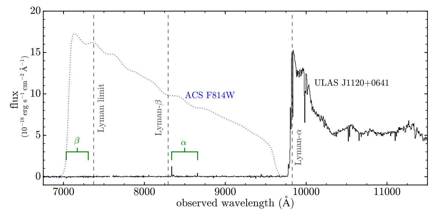 Figure 1
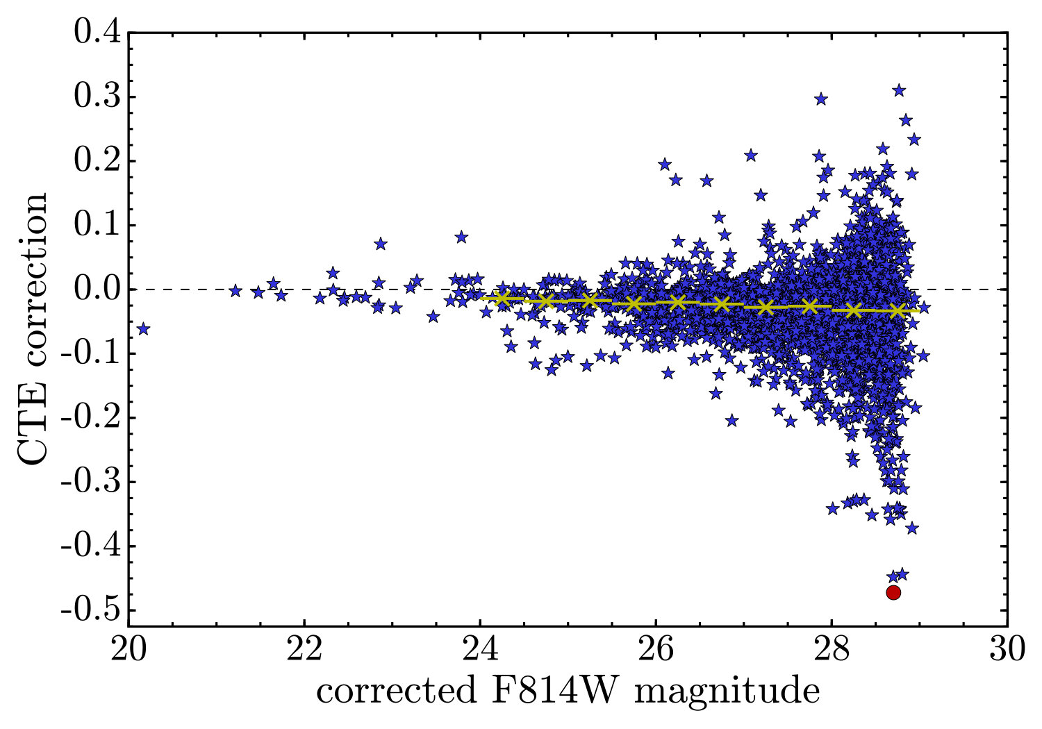 Figure 2
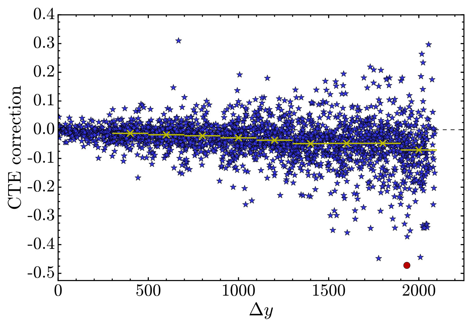 Figure 3
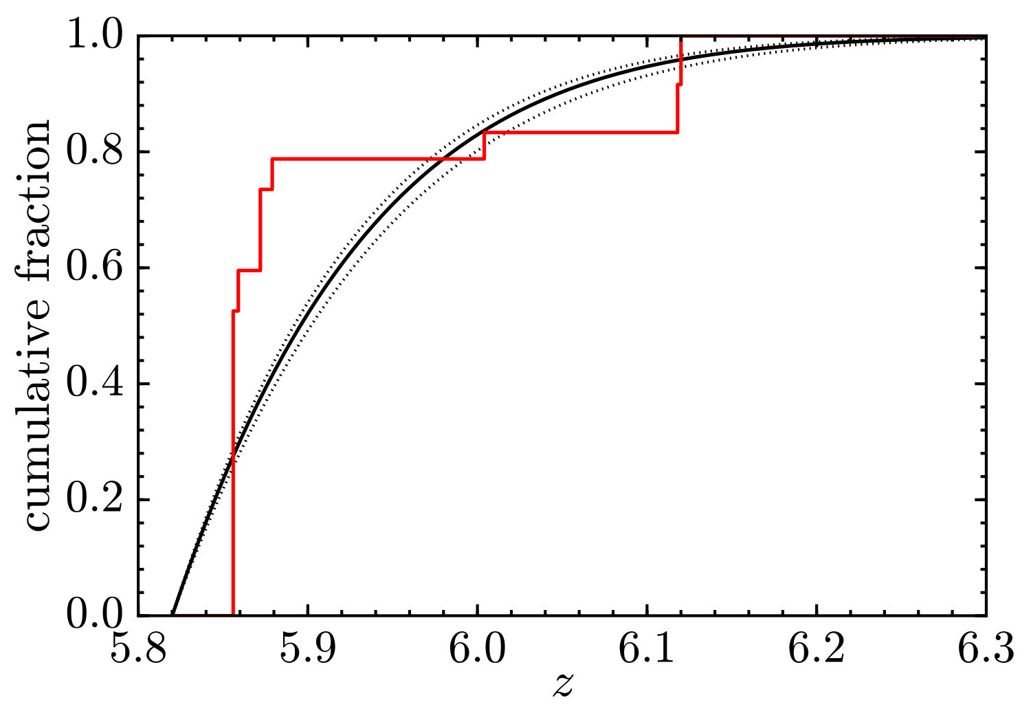 Figure 4
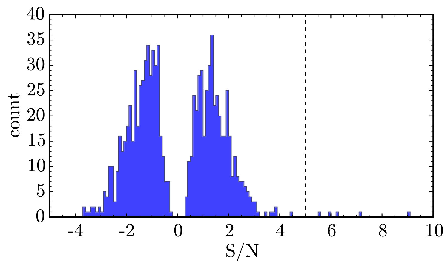 Figure 5
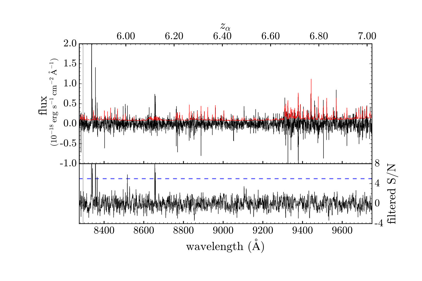 Figure 6
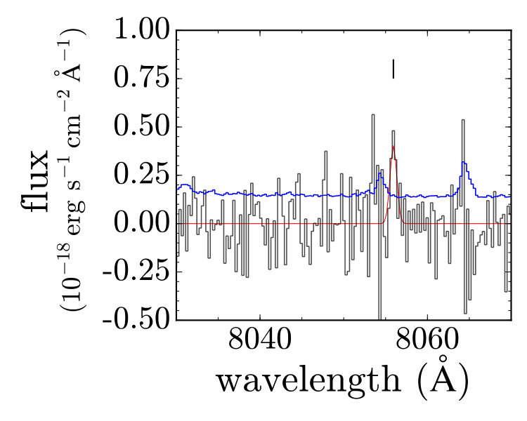 Figure 7
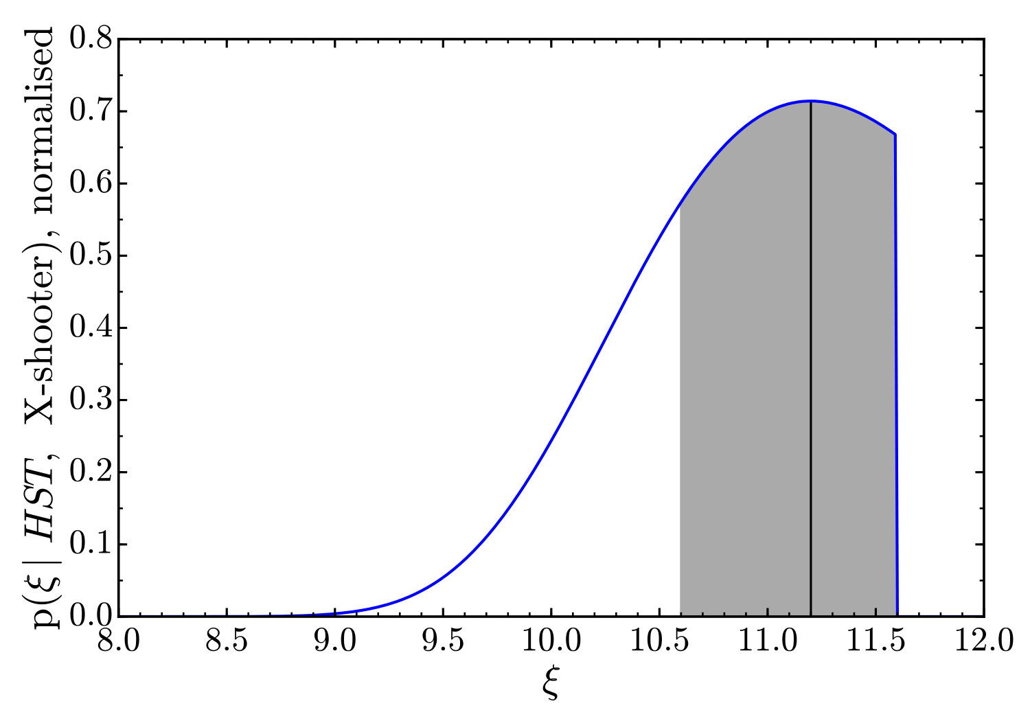 Figure 8
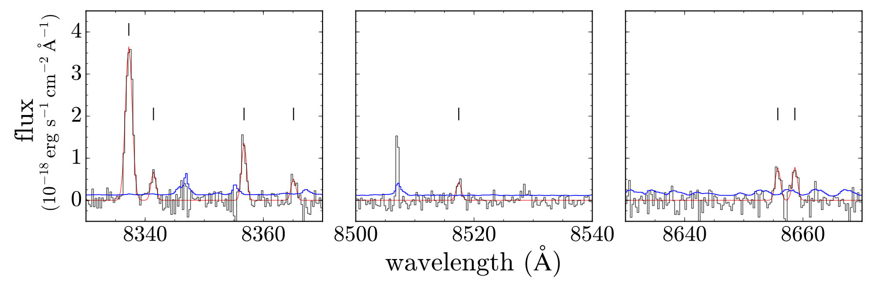 Figure 9
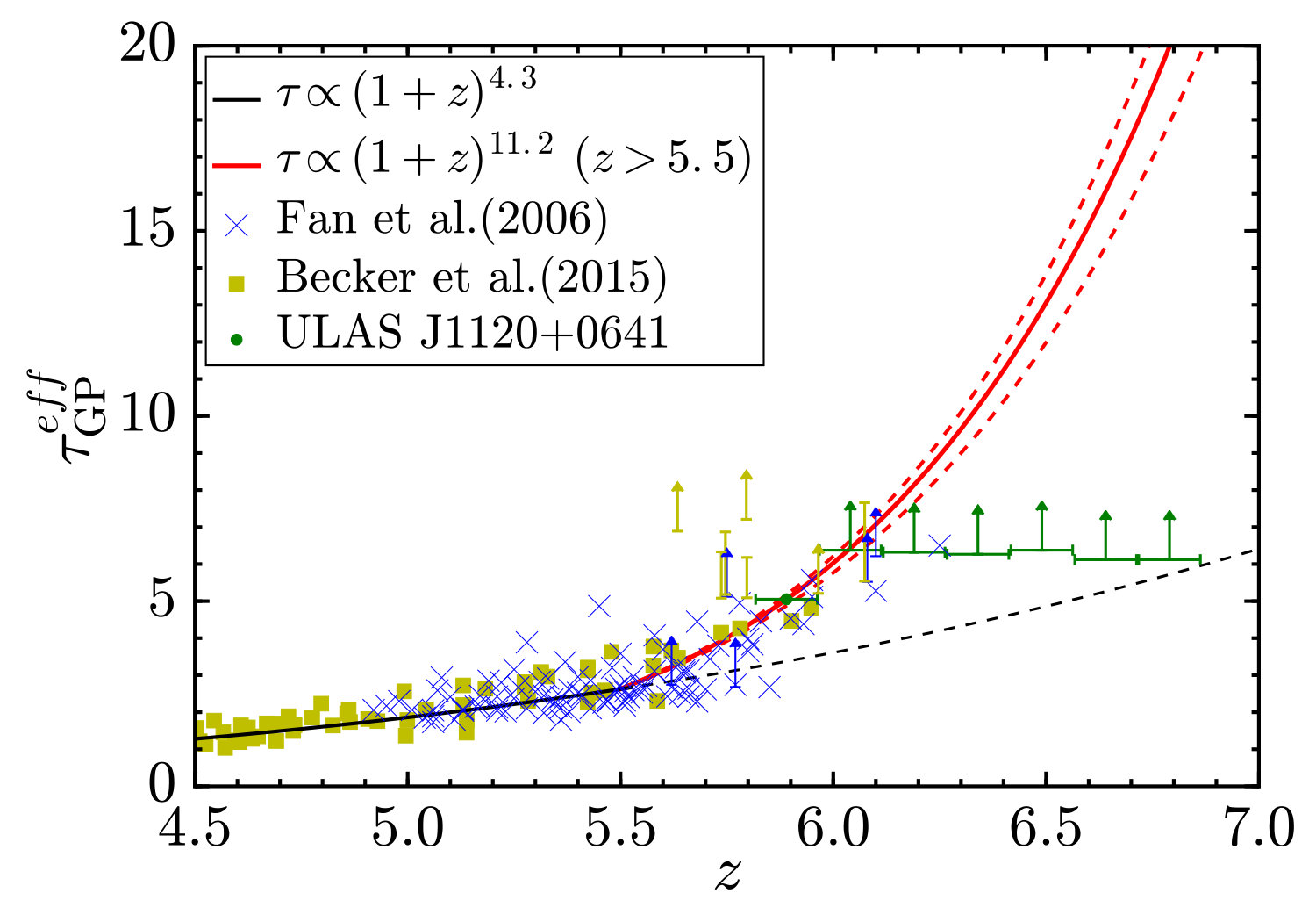 Figure 10
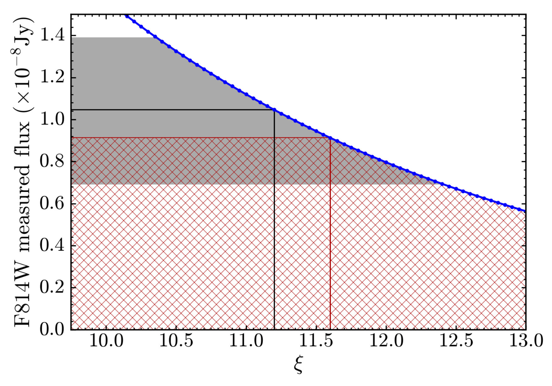 Figure 11
| quasar | redshift range | wavelength range | flux density | ULAS J1120+0641 |
|---|---|---|---|---|
| Å | 10-20 erg s-1 cm-2 Å-1 | 10-20 erg s-1 cm-2 Å-1 | ||
| ULAS J0148+0600 | ||||
| ULAS J0148+0600 | ||||
| SDSS J1030+0524 | ||||
| SDSS J1148+5251 |
| S/N | Spike flux | |||
|---|---|---|---|---|
| Å | km / s | 10-18 erg s-1 cm-2 | ||
| 8337.2 | 5.858 | 21 | 48.7 | 5.34 |
| 8341.4 | 5.862 | 15 | 7.4 | 0.71 |
| 8356.7 | 5.874 | 15 | 14.8 | 1.42 |
| 8365.1 | 5.881 | 15 | 5.6 | 0.54 |
| 8517.4 | 6.006 | 15 | 5.9 | 0.46 |
| 8655.7 | 6.120 | 15 | 9.0 | 0.84 |
| 8658.6 | 6.122 | 15 | 6.2 | 0.85 |
| Å | ||||
|---|---|---|---|---|
| wavelength range | redshift range | bin size | |||
|---|---|---|---|---|---|
| Å | pixels | cMpc | |||
| 732 | 53.6 | ||||
| 635 | 51.7 | ||||
| 698 | 49.9 | ||||
| 682 | 48.3 | ||||
| 666 | 46.6 | ||||
| 653 | 45.2 | ||||
| 638 | 43.7 | ||||
| 625 | 42.4 | ||||
| 612 | 41.1 | ||||
| 600 | 39.9 | ||||
| 589 | 38.8 | ||||
| 576 | 37.5 | ||||
Peer Reviews
No public reviews on file for this paper yet. If you reviewed it on a platform where reviews are public (OpenReview, ICLR, NeurIPS, ICML), you can paste yours below so the community can read it here.
Videos
No videos yet. Explain this paper in a talk, walkthrough, or lecture? Add one.
11institutetext: Astrophysics Group, Blackett Laboratory, Imperial College London, London SW7 2AZ, UK 22institutetext: Department of Physics & Astronomy, University of California, Riverside, 900 University Avenue, Riverside, CA 92521, USA 33institutetext: Department of Mathematics, Imperial College London, London SW7 2AZ, UK 44institutetext: Department of Astronomy, Stockholm University, Albanova, SE-10691 Stockholm, Sweden 55institutetext: Institute of Astronomy, University of Cambridge, Madingley Road, Cambridge CB3 0HA, UK 66institutetext: Kavli Institute for Cosmology, University of Cambridge, Madingley Road, Cambridge CB3 0HA, UK 77institutetext: Gemini Observatory, Northern Operations Center, N. A’ohoku Place, Hilo HI 96720, USA 88institutetext: Max Planck Institut für Astronomie, Königstuhl 17, D-69117 Heidelberg, Germany
Observations of the Lyman series forest towards the redshift 7.1 quasar ULAS J1120+0641
R. Barnett Observations of the Lyman series forest towards the redshift 7.1 quasar ULAS J1120+0641Observations of the Lyman series forest towards the redshift 7.1 quasar ULAS J1120+0641
S. J. Warren Observations of the Lyman series forest towards the redshift 7.1 quasar ULAS J1120+0641Observations of the Lyman series forest towards the redshift 7.1 quasar ULAS J1120+0641
G. D. Becker Observations of the Lyman series forest towards the redshift 7.1 quasar ULAS J1120+0641Observations of the Lyman series forest towards the redshift 7.1 quasar ULAS J1120+0641
D. J. Mortlock Observations of the Lyman series forest towards the redshift 7.1 quasar ULAS J1120+0641Observations of the Lyman series forest towards the redshift 7.1 quasar ULAS J1120+0641Observations of the Lyman series forest towards the redshift 7.1 quasar ULAS J1120+0641Observations of the Lyman series forest towards the redshift 7.1 quasar ULAS J1120+0641Observations of the Lyman series forest towards the redshift 7.1 quasar ULAS J1120+0641Observations of the Lyman series forest towards the redshift 7.1 quasar ULAS J1120+0641
P. C. Hewett Observations of the Lyman series forest towards the redshift 7.1 quasar ULAS J1120+0641Observations of the Lyman series forest towards the redshift 7.1 quasar ULAS J1120+0641
R. G. McMahon Observations of the Lyman series forest towards the redshift 7.1 quasar ULAS J1120+0641Observations of the Lyman series forest towards the redshift 7.1 quasar ULAS J1120+0641Observations of the Lyman series forest towards the redshift 7.1 quasar ULAS J1120+0641Observations of the Lyman series forest towards the redshift 7.1 quasar ULAS J1120+0641
C. Simpson Observations of the Lyman series forest towards the redshift 7.1 quasar ULAS J1120+0641Observations of the Lyman series forest towards the redshift 7.1 quasar ULAS J1120+0641
B. P. Venemans Observations of the Lyman series forest towards the redshift 7.1 quasar ULAS J1120+0641Observations of the Lyman series forest towards the redshift 7.1 quasar ULAS J1120+0641
(Received ¡¿ / Accepted ¡¿)
We present a 30 h integration Very Large Telescope X-shooter spectrum of the Lyman series forest towards the quasar ULAS J1120+0641. The only detected transmission at is confined to seven narrow spikes in the Ly forest, over the redshift range , just longward of the wavelength of the onset of the Ly forest. There is also a possible detection of one further unresolved spike in the Ly forest at , with . We also present revised Hubble Space Telescope F814W photometry of the source. The summed flux from the transmission spikes is in agreement with the F814W photometry, so all the transmission in the Lyman series forest may have been detected. There is a Gunn-Peterson (GP) trough in the Ly forest from all the way to the quasar near zone at . The trough, of comoving length Mpc, is over twice as long as the next longest known GP trough. We combine the spectroscopic and photometric results to constrain the evolution of the Ly effective optical depth () with redshift, extending a similar analysis by Simpson et al. We find where , for . The data nevertheless provide only a weak limit on the volume-weighted hydrogen intergalactic (IGM) neutral fraction at , , similar to limits at redshift from less distant quasars. The new observations cannot extend measurements of the neutral fraction of the IGM to higher values because absorption in the Ly forest is already saturated near . For higher neutral fractions, other methods such as measuring the red damping wing of the IGM will be required.
Key Words.:
ULAS J1120+0641
1 Introduction
It is now over 50 years since Gunn & Peterson (GP; 1965) noted the lack of Lyman- (Ly) absorption in the spectra of (at the time) high redshift quasars. The cross-sections of the Lyman series transitions are so high that even a small neutral hydrogen fraction () should result in an intergalactic medium (IGM) that is effectively opaque to photons at wavelengths shorter than that of Ly emission, 1215.67 Å. However, using observations of the quasar 3C 9 (Schmidt, 1965), Gunn & Peterson (1965) were able to demonstrate an extremely low density of neutral hydrogen ) in the IGM near .
More recently, the Ly forest has been used to constrain the end of reionization by attempting to measure the extent of Ly absorption at redshifts of around six. The lack of GP troughs in the spectra of SDSS quasars with (e.g. Fan et al., 2000, 2001; Djorgovski et al., 2001; Songaila & Cowie, 2002) indicated that the IGM was highly ionized, since a low volume weighted neutral fraction () would be sufficient to result in complete absorption of Ly photons. The first GP trough was reported by Becker et al. (2001) towards the quasar SDSS J1010+0524 (see also White et al., 2003). They concluded that the neutral fraction must increase sharply at .
A seminal study of Lyman series absorption was that of Fan et al. (2006a, see also ), who presented the largest individual sample of high redshift quasars to date. From the spectra of 19 sources, they noted a sharp increase in the effective optical depth to Ly photons (). Their conclusion was that there is an acceleration of the evolution of the IGM ionization state at . Importantly, Fan et al. (2006a) reported a large line-of-sight dependence, indicating patchiness in the IGM neutral fraction that could be related to cosmic reionization. Fan et al. (2006a) also measured a dramatic increase in the average length of dark gaps (in this case defined as contiguous regions with optical depth ) for , suggesting that Ly troughs could be a powerful probe of the IGM at higher redshifts.
The detection of a Mpc GP trough covering the redshift range in the Ly forest towards the quasar ULAS J0148+0600 by Becker et al. (2015) recently strengthened the case for patchiness. Comparing the observations to hydrodynamical simulations, they argue that significant fluctuations in the hydrogen neutral fraction as late as 5.6 - 5.8 are required to explain the data .
Measurements of dark pixels in the Ly and Ly forests have also been used to place the first model independent constraints on reionization. Rather than attempting to measure optical depths based on a continuum model, Mesinger (2010) proposed a novel approach, where the fraction of pixels that have zero measured flux in both Ly and Ly is used to directly measure an upper limit to the volume-weighted mean neutral hydrogen fraction. Applying the idea to observed spectra, McGreer et al. (2011, 2014) conclude that reionization must be (almost) complete by .
The most recent optical depth measurements from Planck, integrated to the last scattering surface (), yield , suggesting a model-dependent redshift of reionization between and ( Collaboration XLVI; Collaboration XLVII 2016).
These various results both from spectroscopic analyses and Planck motivate extending observations of Ly absorption to higher redshifts. ULAS J1120+0641 (Mortlock et al., 2011) remains the only known quasar with (; Venemans et al. 2012). In this paper we analyse the Ly forest towards ULAS J1120+0641 by combining Hubble Space Telescope (HST) imaging from the Advanced Camera for Surveys (ACS), first presented by Simpson et al. (2014), with new spectroscopy from the Very Large Telescope (VLT)/X-shooter instrument (Vernet et al., 2011). The spectrum of ULAS J1120+0641 is shown in Fig. 1. In Sect. 2 we present the data, paying close attention to the effects of charge transfer efficiency (CTE) losses in the case of HST. We remeasure the ACS F814W (-band) image of the quasar. In Sect. 3 we analyse the X-shooter spectrum. We discuss the limitations of spectroscopy for determining optical depth measurements towards the source, and search for significant transmission in the spectrum. In Sect. 4 we combine our photometric and spectroscopic measurements in order to constrain the evolution of effective optical depth towards the quasar, and use simulations to set limits on . We summarise in Sect. 5.
All magnitudes are on the AB system (Oke & Gunn, 1983). We have adopted a concordance cosmology with = 0.7, = 0.3, and = 0.7.
2 Observations and data reduction
2.1 VLT X-shooter spectroscopy
The source was observed with the X-shooter spectrograph over several nights spanning 2011 March to 2014 April, providing a total of 30 h integration on source111ESO programmes 286.A-5025(A), 089.A-0814(A), and 093.A- 0707(A). The Visual-red (VIS) arm of X-shooter, with MIT/LL CCD detectors, spans the wavelength range 5500 - 10000 Å, and the Near-IR arm (NIR), with a Hawaii 2RG array detector, spans the wavelength range 10000 - 25000 Å, or 1.0 - 2.5 m. The quasar’s Ly emission line lies at 9827 Å, close to the boundary between the two arms. In the current paper we analyse the Lyman series absorption in the spectrum, i.e., the wavelength range from the quasar Lyman limit at 7371 Å up to the Ly emission line. This wavelength range lies entirely within the VIS arm.
The data reduction, including flux calibration, is described more fully in Bosman et al. (2017), who provide the spectrum redward of Ly, and present the results of a search for metal lines in that region. Briefly, sky subtraction was performed using a custom idl implementation of the optimum sky subtraction routines outlined in Kelson (2003). This approach involves transforming the CCD coordinates into a wavelength and slit position for each pixel in the two-dimensional frame. Slit positions for each order were defined using a standard star trace. In orders where the quasar has little flux, such as in the Ly forest, the offset from the standard trace and the spatial profile of the object were extrapolated from orders where flux is present, assuming that there is minimal atmospheric dispersion between orders222The majority of our data were acquired in 2013 and 2014, when the X-Shooter atmospheric dispersion corrector was not in use.. This assumption is reasonable given that the Ly forest for ULAS J1120+0641 falls at fairly red wavelengths, and because the object was generally observed at moderate airmass (less than 1.5). Optimal techniques (Horne, 1986) were used to extract a one-dimensional spectrum simultaneously from all exposures for a given spectrograph arm after a relative flux calibration was applied to each order in the two-dimensional frames.
Great care was taken to minimise bias in the sky-subtraction stage of the data reduction, since we are interested in measuring the degree of absorption in the Lyman series forest relative to the continuum. Systematics, where the sky level to subtract is consistently over- or under-estimated, are more important for ULAS J1120+0641 than for several of the other high-redshift quasars used for measuring transmission in the Ly forest because the source is fainter. For example, three quasars in which long GP troughs have been detected, ULAS J0148+0600, (Becker et al., 2015), and SDSS J1030+0524, and SDSS J1148+5251, (White et al., 2003), are respectively factors 3.9, 2.1, and 2.9 brighter than ULAS J1120+0641. Subtle systematics can be present depending on the algorithm used. For example, a weighted least squares fit to the sky where the variance is a Poisson estimate based on the measured counts will systematically underestimate the sky and so leave a positive residual (see White et al. 2003 for a related discussion). To avoid such a bias, we instead used a least-squares linear fit. Likewise, combining multiple exposures using inverse variance weighting can produce a small positive bias when the variance is calculated using a Poisson estimate based on amplitude of the sky fit (plus a contribution from read noise). The bias occurs because exposures in which the sky is underestimated (and hence the object flux overestimated) at a particular wavelength will be assigned a lower variance, and hence a larger weight. To mitigate this bias, we estimated the variance as a function of wavelength using the measured scatter in the two-dimensional counts about the sky fit. A Poisson contribution from the object, based on the extracted counts, is also added along the object trace.
The observations were made with a 09 slit width, providing a nominal resolving power of , or a resolution of 34 km s*-1*. Inspection of the telluric absorption lines, however, indicates that the true mean resolving power was somewhat better, , or a resolution of 30 km s*-1*, as a consequence of good average seeing during the observations. The bin size used for the final spectrum is 10 km s*-1*. The spectrum was flux calibrated using observations of a spectrophotometric standard. Due to slit losses the zero point (i.e. overall scaling) will be uncertain. Accordingly the spectrum was then scaled by matching to the GNIRS spectrum presented in Mortlock et al. (2011) over the region of overlap, redward of the Ly forest, 9800 - 10000 Å. The GNIRS spectrum itself was calibrated to UKIRT photometry, from 2011. The quasar was observed in 2013 March with HST (Sect. 2.2) in the F814W, F105W, and F125W filters (Simpson et al., 2014), and found to have faded by 0.16 mag. compared to the UKIRT photometry. Because we use the F814W photometry in our analysis of the Ly forest, we have applied this additional flux correction to the spectrum, meaning that the normalisation differs from that used by Bosman et al. (2017).
The new X-shooter spectrum is presented in Fig. 1, binned to a pixel size of 150 km s*-1*. As detailed below, the only detectable transmission over the entire Lyman series is confined to the small range in wavelengths marked by in Fig. 1, corresponding to the redshift range 5.858 - 6.122, in the pure Ly forest, and just redward of the onset of the Ly forest, at . The remainder of the Ly forest from up to the edge of the quasar near zone at is completely absorbed, as is the entire region of the Ly and higher series, down to the Lyman limit. The bin width of 150 km s*-1* in Fig. 1 was chosen to emphasise the GP absorption in the plot.
We checked the computed error spectrum by analysing the distribution of signal-to-noise (S/N) ratio in pixels in the long GP trough. We first subtracted off any large-scale systematic residual (Sect. 3.1) using a 301 pixel median filter, before calculating the S/N ratios. We applied a clip and fit a Gaussian to the resulting histogram, which should have a dispersion of unity if the errors are correct. We bin the data for this particular analysis, e.g., by factors of 2, 4, etc., to account for the slight smoothing at the pixel-to-pixel level introduced by rebinning at the wavelength calibration stage. Scaling the noise array by a factor of 1.05 resulted in a Gaussian fit to the residuals with a dispersion of unity. As noted by Bosman et al. (2017), the sky subtraction is imperfect close to the peak of the brightest OH sky lines. Again fitting a Gaussian to the S/N histogram for pixels close to the peak of strong lines, we were able to treat the imperfect sky subtraction by further increasing the errors by a factor of 1.15 for the five pixels centred on each skyline peak.
The errors are on average substantially smaller than in the spectra of the three quasars listed earlier. For example compared to ULAS J1120+0641, in the GP troughs in the spectra of ULAS J0148+0600, , SDSS J1030+0524, , and SDSS J1148+5251, , measured over the same wavelength regions, the errors are on average larger by factors 1.6, 2.5, and 1.8, respectively (consistent with the difference in integration times).
2.2 HST imaging
HST observed the field of ULAS J1120+0641 with the ACS and WFC3 instruments in the three filters F814W, F105W, and F125W, during 2013 March (Simpson et al., 2014). As shown in Fig. 1 the wavelength range of the ACS F814W filter rather neatly spans the Lyman series forest of ULAS J1120+0641, and so photometry of ULAS J1120+0641 in this filter provides valuable information on the Lyman series absorption. The F814W image had a total exposure time of 28,448s spread across five visits made over 2013 March 27–29; it is substantially deeper than the Subaru -band image presented in Barnett et al. (2015). Each visit comprised six dithered exposures, with the exception of the final visit where a single exposure was taken. The 25 pipeline-processed frames were then combined using the pyraf routine astrodrizzle.
Simpson et al. (2014) measured for ULAS J1120+0641 with aperture photometry, using the result to constrain the evolution of the effective optical depth towards the quasar (Sect. 4.1). The source is close to the limit of detectability, and in ACS images the effect of charge transfer efficiency (CTE) losses can be important for such faint sources. As the counts in a detected source are clocked down to the serial register, some charge gets left behind and appears in a trail after the source (Anderson & Bedin, 2010; Chiaberge, 2012). The problem is more severe the lower the background and proportionally greatest for the faintest sources, increasing linearly with distance of the source from the serial register, i.e., with the parallel clocking distance. The placement of ULAS J1120+0641 close to the centre of the field of view of the ACS instrument unfortunately means that the object lies at the edge of one of the CCDs. The distance to the serial register is maximised, as is the charge loss. Therefore, it is important to assess the effect of CTE losses on the photometry.
Two solutions to the problem of CTE losses have been devised by the ACS team. The first (Chiaberge, 2012) quantifies the losses as a function of sky background, source brightness, and location on the CCD, and provides formulae to correct measured photometry. The second (Anderson & Bedin, 2010) attempts to put the trailed charge back into the sources, by applying an ingenious algorithm that uses a model for the CCD traps (defects) that cause the CTE losses. The latter method has proved so successful that it is now applied by default in the ACS data reduction pipeline (although there is an option to turn it off), and the image measured by Simpson et al. (2014) was corrected in this manner.
ULAS J1120+0641 is located close to the ecliptic, resulting in a comparatively bright sky background. In a single frame the average sky level in our F814W frames is 105. This is a considerably higher background than the levels explored by Chiaberge (2012). As the background level rises the CTE corrections become smaller, and the coefficients provided by Chiaberge (2012) allow one to estimate the background level at which the CTE correction becomes zero. Although it becomes necessary to extrapolate their results, the level is , implying that any CTE corrections in our frames should actually be very small. We consulted with the ACS instrument team on the issue of the CTE correction, and they recommended that at such high background levels losses should indeed be small, and that we should use frames without the Anderson & Bedin (2010) corrections applied, since for high background the algorithm will simply add noise.
As a check, we used astrodrizzle to produce co-added frames of the dithered F814W exposures both with and without the Anderson & Bedin (2010) correction in order to quantify the CTE corrections made as a function of source brightness, and of location on the CCD. We paid close attention to the choice of input parameters to astrodrizzle to avoid the cores of bright objects being masked as cosmic rays. We used SExtractor (Bertin & Arnouts, 1996) to produce a catalogue of objects in the HST frames, detected in the corrected F814W image. We performed aperture photometry at the positions specified by the catalogue in both the corrected and uncorrected F814W images. Ideally the sample would be restricted to point sources, but star/galaxy discrimination is unreliable for sources as faint as ULAS J1120+0641, so we included all catalogued sources. CTE corrections for galaxies will be larger than for point sources, as they cover more pixels, so any measured trends may in fact overestimate the CTE correction for a point source. The centroid of the image of ULAS J1120+0641 is also uncertain as the source is so faint. We therefore used the F105W frame to define the position of the quasar, before measuring photometry in the two F814W frames. However, the F105W proved a poor choice to define the whole catalogue, as it is shallower than the F814W observation and so fewer objects were detected. Finally, we calculated the CTE corrections for all sources. These are presented as a function of corrected magnitude in Fig. 2a, and of the distance in pixels from the serial register, , in Fig. 2b. In each of these plots very weak trends, at the level of few hundredths of a magnitude are visible in the mean correction for all objects at a particular magnitude or clocking distance, but these are much smaller than the standard deviation. Furthermore, as noted above, these trends may overestimate the required correction, as the sample is dominated by galaxies. We conclude that when the background is this high the Anderson & Bedin (2010) algorithm simply introduces additional noise, and the best photometry is provided by the uncorrected frame. The correction for ULAS J1120+0641 itself is large: the quasar lies in the tail of the distributions and is brightened by 0.47 mag. This unusually large correction appears to be due to chance.
The uncorrected frame has a stripy appearance from (fractionally small) CTE losses in bright sources. Therefore, we flattened the sky background before aperture photometry by subtracting a median-filtered version of the frame. We measured the counts in a 3-pixel radius (rather than the 2.5 pixel aperture preferred by Simpson et al. 2014, to minimise digitisation issues), and applied an aperture correction to 10 pixel radius (), derived from bright stars. This was then further corrected to the nominal “infinite” aperture radius of the ACS of using the quoted encircled energy fraction of 0.914 in the aperture, quoted in the ACS Data Handbook. The final photometry result is , with . We quote the error as a signal-to-noise ratio as the errors are Gaussian in flux, but at such low significance the equivalent posterior distribution in magnitudes is extremely skewed, and we do not quote it here.
3 Analysis of the spectrum
3.1 Systematic errors in sky subtraction
In exploring the Ly forest in the new spectrum, smoothing on different scales, we found that despite the care taken in the data reduction to minimise such effects (Sect. 2.1), there are systematic errors present in the form of a small positive residual signal at an average level of erg s*-1* cm*-2Å-1*. The excess corresponds to only of the counts from the sky within the extraction aperture, or of the average random error per pixel. We used synphot (Laidler et al., 2008) to measure synthetic photometry from the spectrum, obtaining a value , which is a factor 4.5 brighter than the HST photometry. The low-level sky residual is difficult to characterise quantitatively, since a detection alone requires binning over 400 pixels ( Å). However, the residual does not correlate directly with the error spectrum, in the sense that on large scales they do not share the same shape. Neither is the residual significantly greater in the wavelength ranges of the bands of OH sky lines, compared to the line-free regions. Therefore it does not seem to be an effect associated with the difficulty of subtracting the sharp OH sky lines, and is apparently a smooth feature.
Systematic errors in sky subtraction have not been reported or quantified in previous measurements of the Lyman-series effective optical depth. We checked whether a residual at the level seen in the spectrum of ULAS J1120+0641 would have been detected in the GP troughs seen in the spectra of the three quasars ULAS J0148+0600 (Becker et al., 2015), SDSS J1030+0524, and SDSS J1148+5251 (White et al., 2003). In these papers, the transmission in the GP troughs is measured in bins of width Mpc, and transformed to an effective optical depth. Using the same bins we have measured the average flux density in the spectra, using inverse-variance weighting, and the results are provided in the fourth column of Table 1. In three of the bins the measured flux is consistent with zero, while significant flux is recorded in the GP trough in the spectrum of SDSS J1148+5251. We then measured the average flux density over the same four bins in the spectrum of ULAS J1120+0641, after subtracting the few transmission spikes seen in the spectrum (Sect. 3.2), in order to measure the smooth residual. These results are listed in the final column of Table 1. In the spectrum of ULAS J1120+0641 we measure significant flux at the level of erg s*-1* cm*-2Å-1* in all four bins.
The detection of significant flux in the redshift bin in the spectrum of SDSS J1148+5251 is interesting, because it is the only other case where significant flux has been measured where no transmission spikes in Ly have been detected. In the original paper, White et al. (2003) speculated that this was due to flux from a faint intervening galaxy, a suggestion which has subsequently been ruled out by HST imaging (White et al., 2005). Systematic errors in the sky subtraction may provide a simpler explanation. In fact, comparing the values in columns 4 and 5 of Table 1, in each bin the measurements agree at the level. This means that systematic errors could be present in the other spectra at a similar level, and the reason they are reported here for the first time is because it is the deepest spectrum yet taken at these redshifts.
3.2 Detection of transmission spikes
To remove the systematic residual we subtracted a median-filtered version of the spectrum using a box of length 301 pixels, i.e., Å. At these redshifts transmission in the Lyman-series forest will be in isolated spikes, so the application of a median filter of such a long box length should have a negligible effect on any inferred transmission. The region of the spectrum covering the Ly forest, binned by a factor two for display purposes, i.e., pixels of 20 km s*-1*, is shown in Fig. 3, together with the error spectrum. Note, however, that we use the unbinned spectrum to search for regions of significant transmission. To search for spikes in the Lyman series forest () we employ a Gaussian matched filter (Hewett et al., 1985; Bolton et al., 2004), with a range of widths. The narrowest profile has a standard deviation km s*-1*, corresponding to the nominal spectral resolution of 34 km s*-1* FWHM. A range of profiles successively increasing in width by was employed, , 21, 30, …, 120 km s*-1*. We fit a Gaussian at every pixel, 8535 in total. To illustrate the process we plot the S/N at each pixel for the narrowest template in the bottom panel of Fig. 3. Then, for each pixel, we recorded the of the most significant detection over all the templates, whether positive or negative, and the corresponding value of .
The distribution of these S/N values is shown in Fig. 4. This distribution is non-Gaussian, because we recorded the maximum absolute value for each pixel. Since negative spikes, which are not real, extend down to nearly , we cannot be sure positive spikes are real unless the S/N is substantially greater than 4. In fact one might expect a somewhat more extended tail in the positive direction, of spikes that are not real, because of cosmic rays that are not perfectly subtracted. For these reasons we set our detection threshold at . The matched filter finds seven significant flux transmission spikes, at observed wavelengths , redshifts . These are summarised in Table 2 and plotted in Fig. 5. These seven spikes are also identifiable in both panels of Fig. 3. To confirm that the detections are real, for each spike we compared the measured flux at the detected wavelength in subsets of the data, and found no significant differences between subsets. We also checked the goodness of the fit of the Gaussian template to the data, finding the values to be satisfactory. The observed transmission features are very narrow: with the exception of the largest spike at 8337 Å, the template width which yielded the highest S/N was 15 km s*-1*, i.e., the spikes are unresolved. We integrate the template transmission spectrum to find a total transmitted flux of () erg s*-1* cm*-2*, of which approximately half is contained in the largest spike.
Using synphot we measure for these seven spikes. Our value is consistent with the HST photometry (Sect. 2.2; , ), raising the question of whether the seven spikes account for all the transmission in the spectrum. In considering this question we refer to Table 3 which sets out the wavelength ranges in the spectrum and the corresponding redshifts over which absorption in the four transitions Ly, , , are recorded. It is noticeable that the seven spikes all lie close to the blue end of the pure Ly forest, which is to be expected. Starting at the red end of the Ly forest, on the edge of the quasar near zone (near 9770 Å), and moving to shorter wavelengths, the Ly opacity reduces, down to 8291 Å, , where the high-opacity Ly forest at cuts in. Moving to shorter wavelengths from 8291 Å the opacity in Ly becomes lower, but will still be very high at 7862 Å, corresponding to , at which point the Ly forest cuts in at . The result is that the most transparent window in the spectrum is just redward of 8291 Å. Therefore if there is any more transmitted flux in the spectrum, which will be in the form of narrow spikes below significance, most of it is expected to lie in the wavelength range 8291 - 8700 Å. Looking at the spikes with S/N in the range 3 - 5 these are approximately uniformly distributed along the spectrum, with no excess detected in the wavelength range 8291 - 8700 Å. Even if all the 3 - 5 spikes in this wavelength range were real, they would only contribute an additional to the transmitted flux. The region of Ly absorption corresponding to the transmission spikes, is marked in Fig. 1. It is beyond the quasar Lyman limit, and is consequently not useful for measuring transmission.
There is a single unresolved spike in the range of ambiguity . It is detected at , and lies at , corresponding to and . The spike is plotted in Fig. 6. A region of transmission at would be very unexpected given the rapid evolution of the hydrogen neutral fraction seen around , so the feature is potentially interesting. We checked that the fluxes measured in subsets of the data are consistent. The putative line lies six pixels from the centre of a strong OH sky line, sufficiently far away that it should not be affected by poor sky subtraction. Unfortunately it is not possible to be sure if the line is real or not.
If the spike is real, it requires that the opacities along the line of sight to the quasar at redshifts and are both low. We are able to quantify this statement by following a line of reasoning used by White et al. (2005) in discussing a Ly transmission spike in the spectrum of SDSS J1148+5251. In the spectrum of ULAS J1120+0641, the fractional transmission measured over five pixels centred on the Ly spike is . The effective optical depth at 8056 Å, which is the sum of contributions from both the Ly and Ly forests, is . The transmission at the corresponding wavelength in the Ly forest, , Å, measured over 5 pixels, is (9548), meaning an optical depth at 2. Taking the ratio of effective optical depths from Fan et al. (2006a), the measurement at Å, implies , and . The range on is not unreasonable, meaning that our analysis does not weaken the case that the line is real. Combining the two transmission measurements, and assuming , leads to the constraint for this spike.
3.3 Measurement of the effective GP optical depth
Narrow features are essentially unaffected by the application of the long median filter, and so we use the filtered spectrum to measure the effective optical depth in the Lyman series forest. To normalise the spectrum and hence estimate the transmitted flux ratio , we divide the X-shooter spectrum by the model intrinsic spectrum described in Mortlock et al. (2011). Here the blue wing of the Ly emission line comes from a composite spectrum created from sources with similar CIV blueshifts, and the spectrum is extended bluewards as a power law .
In Table 4 we present measurements of and effective GP optical depth over the redshift range , covering practically the entire Lyman series forest. We follow the prescription of Fan et al. (2006a), making measurements in fixed-size bins of . The redshift bin was excluded as the median filtered spectrum is affected by the quasar Ly emission line in this region. To estimate we calculate the transmission fraction in each pixel before taking the inverse-variance weighted average for each bin, i.e., . If we detect transmission below a level of , we adopt a lower limit for based on a value of equal to twice the uncertainty333 A more elegant approach would be to deduce a posterior probability density function for and hence . The true value of , so by assuming a uniform prior for and a Gaussian likelihood, it would be possible to determine posterior confidence intervals for . By adopting a upper limit for , we have followed the method used to measure existing limits on (e.g. Fan et al., 2006a; Becker et al., 2015). Given that absorption in the Ly forest is saturated at , our choice is ultimately not very important. .
We also consider the effect of the adopted power-law slope at wavelengths below Ly. We recalculate values using a bluer continuum, (Lusso et al., 2015). The effect on is found to be small. In the lowest-redshift bin we find , while in the highest redshift bins the difference is negligible. In the bin beginning at we measure , i.e., consistent with the value presented in Table 4.
In Fig. 7 we show our measurements of , as well as the power law evolution of determined using HST photometry (Sect. 4.1). We do not include the bins for which in Fig. 7, since these have contributions from Ly and higher order transitions, as well as Ly. In principle, observations of Ly in the redshift range might provide a more sensitive measurement of the effective optical depth, if corrected for the coincident absorption by Ly at . Although a statistical correction for foreground Ly is possible at lower redshifts, the recent results of Becker et al. (2015) show that this is not possible at , as some lines of sight are completely absorbed in Ly.
The results for ULAS J1120+0641 lend support to the steadily-growing body of evidence that climbs rapidly at high redshift, and that therefore we are observing the tail-end of the epoch of reionization. However, it is also clear from Fig. 7 that we are unable to make especially useful measurements of for . Absorption in the spectrum becomes saturated, and so no further information can be gained by measuring up to redshifts of seven since we can only determine lower limits which are similar in value to the measurements of from lower redshift sources. As expected, the most useful constraints on come from .
4 Analysis and discussion
4.1 IGM opacity
Fan et al. (2006a) used the spectra of 19 quasars to measure along different lines of sight. They found the best-fit power law to be:
[TABLE]
empirically determining a limit of . We now wish to measure a value of following a procedure similar to that used by Simpson et al. (2014), using our revised photometry. We have an additional constraint on , namely the transmission spikes detected in the X-shooter spectrum.
The intrinsic quasar emission below Ly is modelled using the power law chosen by Mortlock et al. (2011), , which is normalised to the observed spectrum at 1280 Å. Absorption in the IGM is modelled using Equation 1. The wavelength of each pixel is converted to a Ly redshift, which is used to calculate for a particular value of . Measuring the absorbed spectrum with synphot produces a synthetic magnitude that we can compare directly to the F814W result. We show the fluxes measured for a range of values in Fig. 8. Combining the synthetic photometry with spectroscopy, we determine a posterior distribution for , shown in Fig. 9. We have assumed a uniform prior for , and a Gaussian distribution for the measurement which is equivalent to Jy. The sharp cut-off results from determining a lower limit to the flux from the transmission spectrum derived in Sect. 2.1, measured as Jy (AB 29.00, ). Higher values of are excluded, as the resulting measurements are below this secure lower flux limit. The posterior peaks at , for which the synthetic photometry yields the HST result (Fig. 9). The 68% highest posterior density credible interval is shaded, giving . The resulting evolution of is shown in Fig. 7.
4.2 Flux distribution in the Ly forest: the longest GP trough to date
The detected transmission spikes account for )% of the quasar flux detected by HST, with the uncertainty dominated by the photometry measurement. Therefore all of the transmission in the spectrum may have been detected. Even if there are any additional lower-significance transmission features they are likely to be found in the same redshift range and to follow a similar distribution. The shape of the cumulative distribution of the transmitted flux therefore provides a noisy estimate of the shape of the cumulative transmission of the Ly forest, and so it is interesting to compare this to the model.
In Fig. 10 we present the cumulative proportion of flux contained in transmission spikes with redshift i.e. the cumulative transmitted flux as a function of redshift, normalised to the total transmitted flux. The result from spectroscopy is compared to the model derived in Sect. 4.1, which we use to produce an average transmission spectrum. In both cases the distributions are normalised to the total transmitted flux as we wish to compare the relative shapes.
Broadly speaking, the distributions are in good agreement. In particular, our model for predicts effectively zero transmission for , which is consistent with the transmission spectrum.
The distribution of transmission features is consistent with an extremely long GP trough extending to the quasar’s near-zone, covering the redshift range , equivalent to a comoving distance of 240 Mpc. This is more than twice the length of the next longest trough reported by Becker et al. (2015) towards the quasar ULAS J0148+0600, although that trough extends to significantly lower redshifts .
4.3 Constraints on the IGM neutral fraction
Previous studies have used the evolution of the IGM Ly opacity to constrain up to (Fan et al., 2006a; Becker et al., 2015). The large cross-section of Ly means that the forest will be almost completely absorbed by even for (e.g. Fan et al., 2006a), and density evolution will naturally make the IGM even more opaque at . Nevertheless, we wish to determine what we can learn about from the long trough towards ULAS J1120+0641.
In order to constrain we use artificial spectra generated from the Sherwood suite of hydrodynamical simulations, which are described in detail in Bolton et al. (2017). Briefly, they were run using a modified version of the parallel Tree-PM SPH code P-GADGET-3, which is an updated version of the publicly available GADGET-2 (Springel, 2005). The models use a CDM cosmology consistent with recent Planck results ( Collaboration XVI, 2014). Here we use the reference 40 - 2048 model, which uses a 40 Mpc box and particles, giving a gas particle mass of . Reionization occurs at , whereafter the gas temperature and ionization fraction evolve assuming a spatially uniform Haardt & Madau (2012) ionizing ultraviolet background (UVB). Simulation outputs were captured in redshift steps of , and one-dimensional Ly forest skewers were generated from the outputs following standard methods (e.g., Theuns et al., 1998).
Our goal is to set limits on the neutral fraction required to produce the 240 Mpc trough over seen towards ULAS J1120+0641, and we generate mock Ly forest spectra with properties matched to the data using the following approach:
For each trial, six individual 40 Mpc skewers are selected at random from the simulation, with the simulation redshifts chosen to most closely match the observed line-of-sight. 2. 2.
The Ly optical depths () are scaled according to the ratio of our desired to the native in the simulation. 3. 3.
Transmitted fluxes are computed as . 4. 4.
The spectra are smoothed to the nominal instrumental resolution of and binned using 10 km s*-1* pixels, as in the real data. 5. 5.
Random Gaussian noise is added with dispersion given by the ULAS J1120+0641 error spectrum (normalized by a power law fit to the flux redward of the Ly emission line and extrapolated over the forest). 6. 6.
A matched-filter search for transmission peaks is then performed following the procedure described in Sect. 3.2. For efficiency, we use only the narrowest filter width (), although our results are not highly sensitive to this choice.
We parametrize the evolution in the neutral fraction as a power law of the form , where is the volume-weighted neutral fraction at , i.e., near the start of the trough. For reference, the simulation has a native evolution given by over the redshift range of interest. We generate mock spectra for each combination of and . Our 95% confidence limits on these parameters are those for which no transmission peaks are detected with in at least 5% of the trials. For , we find . Increasing to 9 gives , which is consistent with using a Haardt & Madau (2012) UVB. The limits on are thus largely insensitive to , as expected if most of the constraining power comes from the low-redshift end of the trough.
In summary, we find that the Ly trough towards ULAS J1120+0641, while remarkably long, provides only a weak lower limit to the volume-weighted neutral fraction of the IGM (), consistent with a highly ionized IGM. The weakness of this constraint is because the trough lies at very high redshift (), where large Ly opacities are more easily produced due to high IGM densities. We note that we have only considered an IGM model with a spatially uniform UVB and temperature-density relation, which implicitly assumes that the most transmissive regions of the IGM will be low-density voids. There is evidence that is significantly patchy on large scales at (Becker et al., 2015). Models that attribute this patchiness to a non-uniform background produced by star-forming galaxies tend to predict that the UVB intensity will be anti-correlated with large-scale density enhancements (Davies & Furlanetto, 2016; D’Aloisio et al., 2016). In these models, the highest transmission tends to come from high-density regions, and thus a lower would be required to produce significant Ly transmission. Alternatively, the patchiness may be due to residual large-scale temperature fluctuations from an extended reionization process (D’Aloisio et al., 2015). In that model, high transmission tends to occur in hot (), low-density regions that have only recently been reionized. Since these regions would be hotter than we have assumed and the neutral fraction scales as , Ly transmission might appear even if the globally-averaged is somewhat larger than our constraint.
The constraints on from the Ly trough towards ULAS J1120+0641 are considerably weaker than those determined from Ly damping wing absorption, first measured by Mortlock et al. (2011), who found at . The most recent Ly damping wing constraints on the volume-weighted neutral fraction come from an analysis of the FIRE infrared spectrometer spectrum of ULAS J1120+0641 (Simcoe et al., 2012) by Greig et al. (2016), who find . Greig & Mesinger (2016) argue that the measured Ly damping wing absorption towards ULAS J1120+0641 provides one of the strongest constraints on reionization that are currently available. As we begin to probe ever-higher neutral fractions, measurements of Ly damping wing absorption will likely provide far more useful constraints than the Ly forest. A further analysis of the damping wing towards ULAS J1120+0641 using the deeper X-shooter spectrum will be presented in Hewett et al. (in prep.).
5 Summary
We have analysed a deep X-shooter spectrum and HST F814W photometry of ULAS J1120+0641 to probe the Ly forest to along the line of sight to the quasar. Our main results are as follows:
We revise F814W photometry of ULAS J1120+0641 to be , with . For a faint source such as ULAS J1120+0641 which is measured against a high background, the Anderson & Bedin (2010) CTE correction included in the ACS pipeline merely introduces noise to the photometry. 2. 2.
Significant transmission in the Lyman series forest is restricted to the redshift range , where seven spikes were detected at . 3. 3.
Photometry provides us with more useful constraints on effective optical depth, while spectroscopy can still be used to derive a lower limit on transmitted flux. Using data for ULAS J1120+0641 alone and assuming a fixed normalization at , for redshifts we find where . 4. 4.
We detect an extremely long dark gap extending from the final transmission spike to the quasar’s near-zone, equivalent to a comoving distance of 240Mpc. The GP trough nevertheless provides only a weak limit on the IGM neutral fraction at confidence. This is a generic limitation of observations of the Ly forest at such high redshifts.
Acknowledgements.
We are grateful to the referee, Michael Strauss, who provided constructive comments and improvements. We would like to thank the ACS instrument team for their helpful guidance on the effects of CTE losses. We also thank Jamie Bolton for the use of the Sherwood simulations. This work was supported by Grants ST/K502042/1 and ST/N000838/1 from the Science and Technology Facilities Council. SJW gratefully acknowledges the support of the Leverhulme Trust through the award of a Leverhulme Research Fellowship. GDB is supported by the National Science Foundation under Grant AST 1615814. PCH and RGM acknowledge support from the STFC via a Consolidated Grant to the Institute of Astronomy, Cambridge. BPV acknowledges funding through the ERC grant “Cosmic Dawn”.
The reference list from the paper itself. Each links out to its DOI / PubMed record.
- 1Anderson & Bedin (2010) Anderson, J. & Bedin, L. R. 2010, PASP, 122, 1035
- 2Barnett et al. (2015) Barnett, R., Warren, S. J., Banerji, M., et al. 2015, A&A, 575, A 31
- 3Becker et al. (2015) Becker, G. D., Bolton, J. S., Madau, P., et al. 2015, MNRAS, 19
- 4Becker et al. (2001) Becker, R. H., Fan, X., White, R. L., et al. 2001, AJ, 122, 2850
- 5Bertin & Arnouts (1996) Bertin, E. & Arnouts, S. 1996, A&AS, 117, 393
- 6Bolton et al. (2004) Bolton, A. S., Burles, S., Schlegel, D. J., Eisenstein, D. J., & Brinkmann, J. 2004, AJ, 127, 1860
- 7Bolton et al. (2017) Bolton, J. S., Puchwein, E., Sijacki, D., et al. 2017, MNRAS, 464, 897
- 8Bosman et al. (2017) Bosman, S. E. I., Becker, G. D., Haehnelt, M. G., et al. 2017, MNRAS, in press