Bayesian Probabilistic Numerical Methods
Jon Cockayne, Chris Oates, Tim Sullivan, Mark Girolami

TL;DR
This paper formalizes Bayesian probabilistic numerical methods as solutions to inverse problems, providing conditions for their well-definition, convergence, and compositional use in complex tasks, bridging numerical analysis and uncertainty quantification.
Contribution
It establishes a rigorous Bayesian framework for probabilistic numerics, including convergence analysis and methods for composing solutions to complex numerical problems.
Findings
Bayesian probabilistic numerical methods are well-defined under general conditions.
A numerical approximation scheme with proven asymptotic convergence is proposed.
The framework is extended to pipelines of computation for complex tasks.
Abstract
The emergent field of probabilistic numerics has thus far lacked clear statistical principals. This paper establishes Bayesian probabilistic numerical methods as those which can be cast as solutions to certain inverse problems within the Bayesian framework. This allows us to establish general conditions under which Bayesian probabilistic numerical methods are well-defined, encompassing both non-linear and non-Gaussian models. For general computation, a numerical approximation scheme is proposed and its asymptotic convergence established. The theoretical development is then extended to pipelines of computation, wherein probabilistic numerical methods are composed to solve more challenging numerical tasks. The contribution highlights an important research frontier at the interface of numerical analysis and uncertainty quantification, with a challenging industrial application presented.
Click any figure to enlarge with its caption.
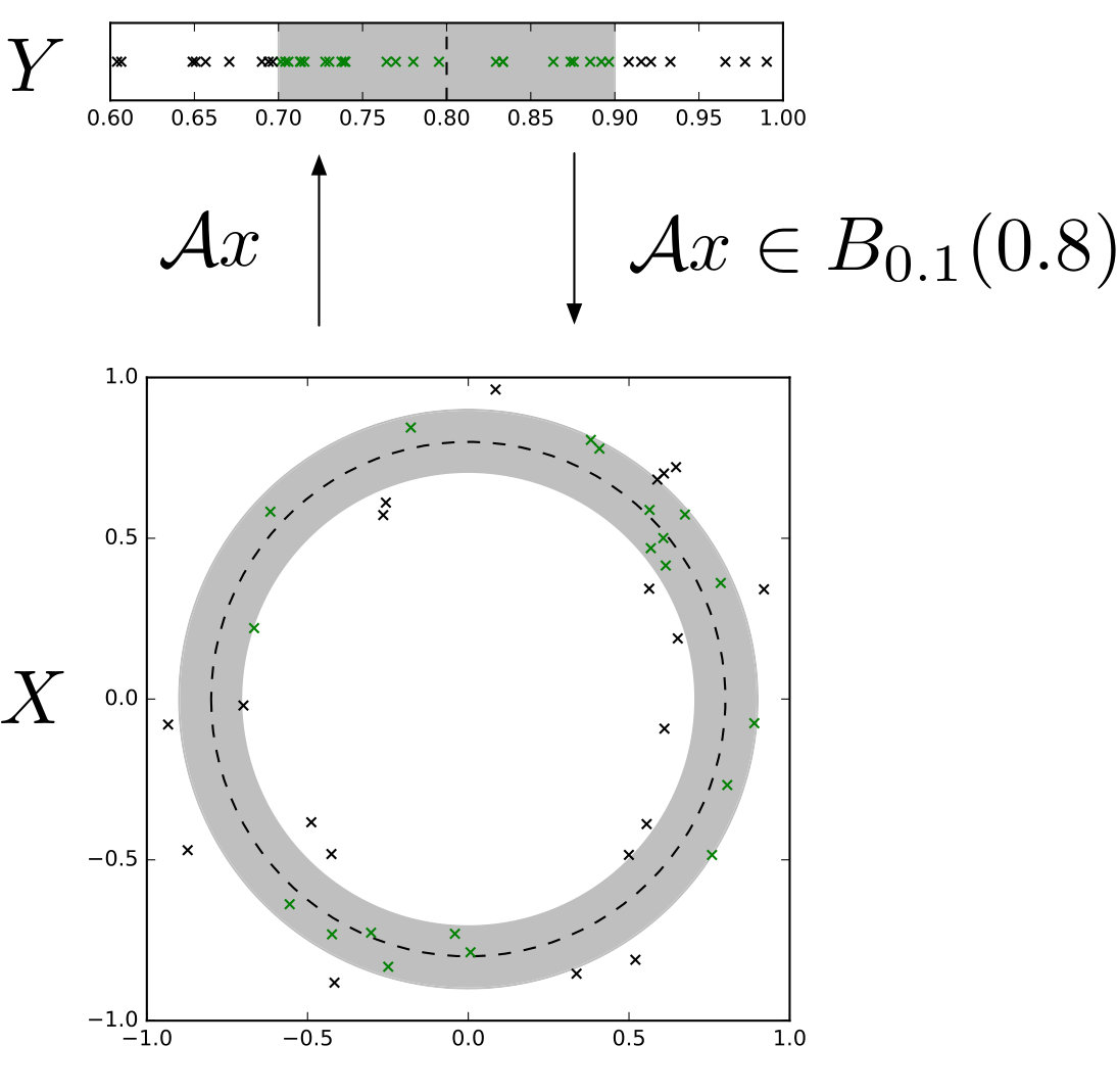 Figure 1
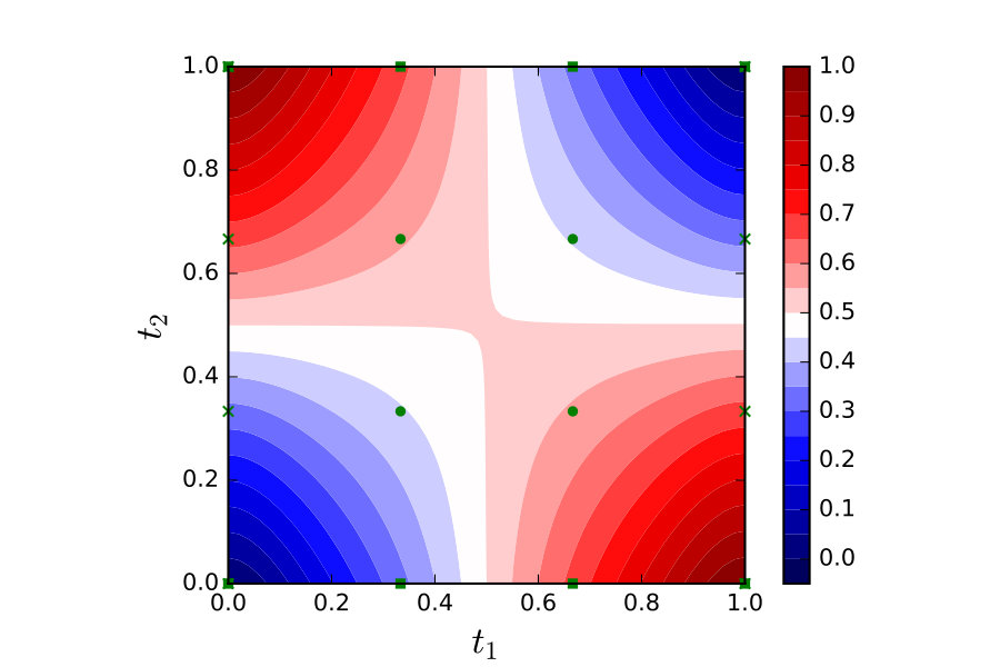 Figure 2
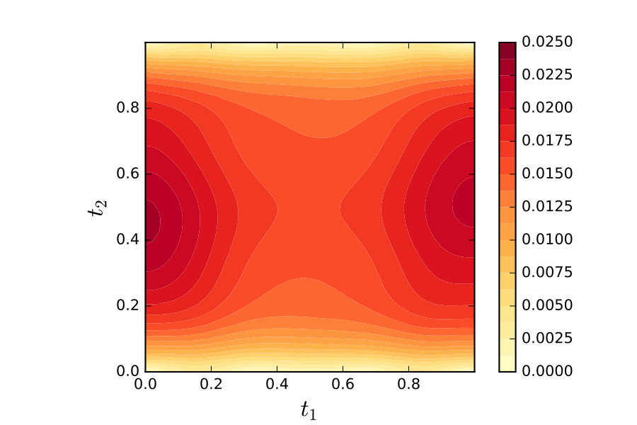 Figure 3
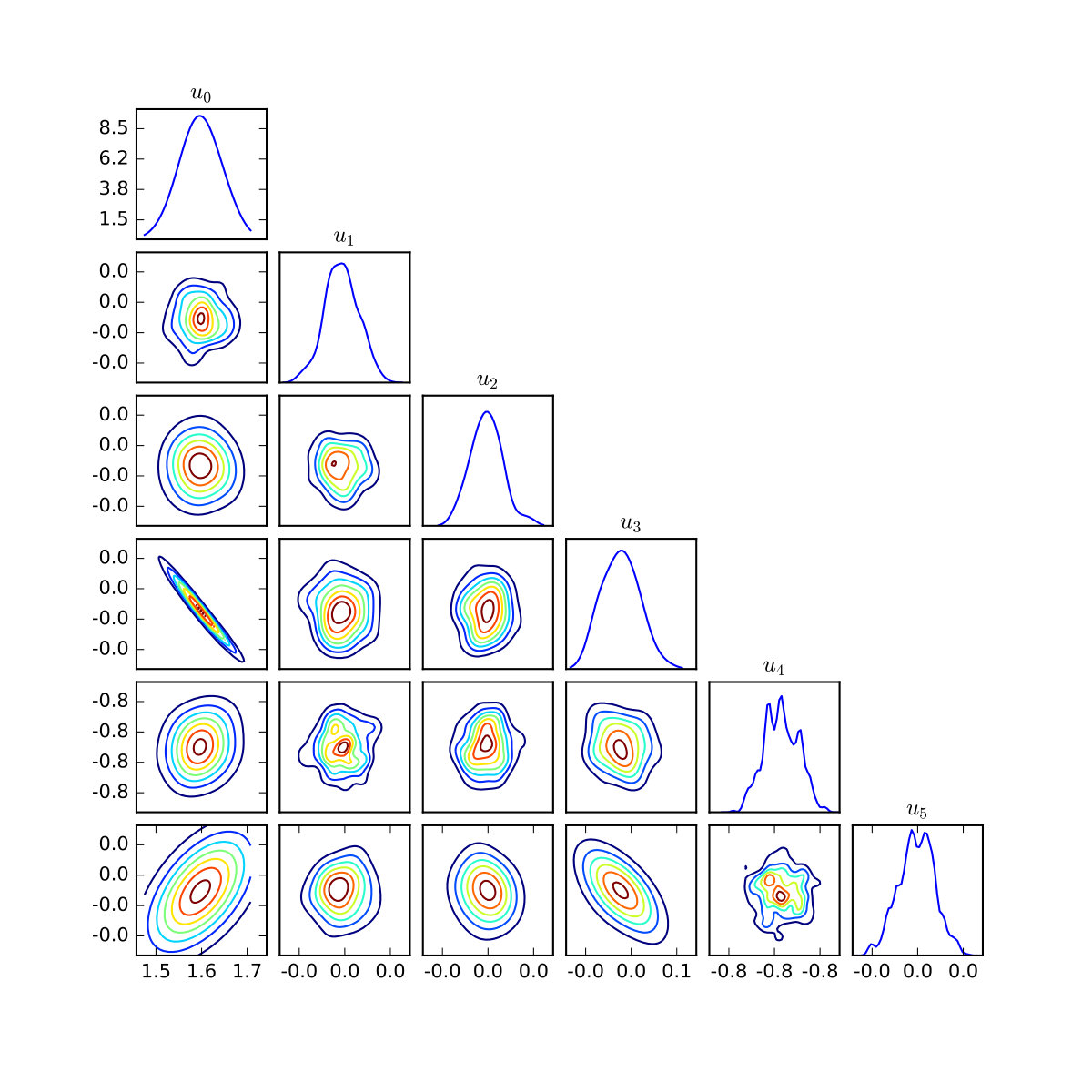 Figure 4
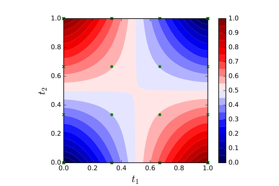 Figure 5
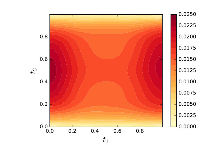 Figure 6
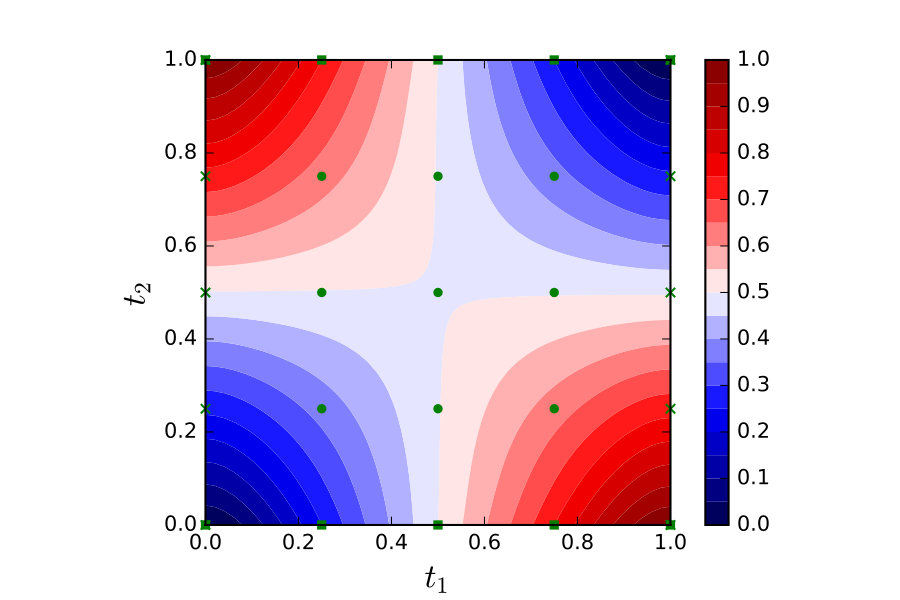 Figure 7
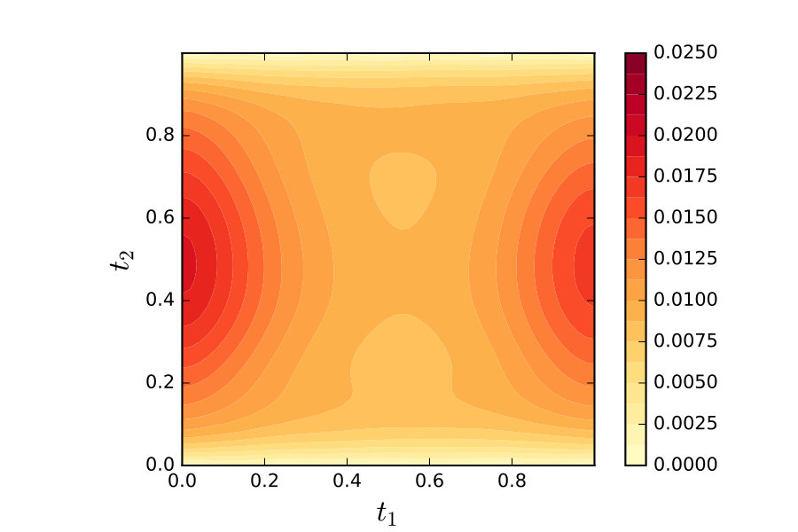 Figure 8
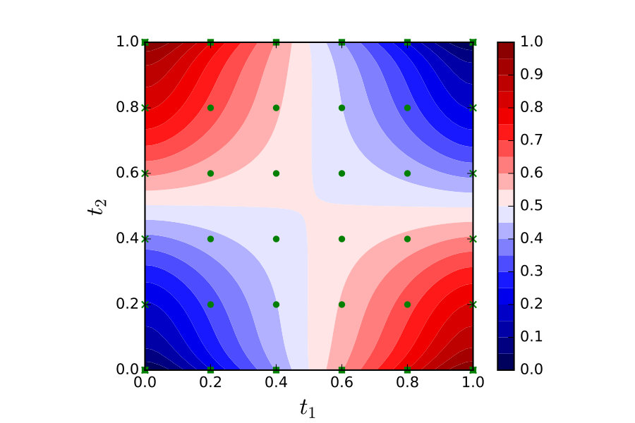 Figure 9
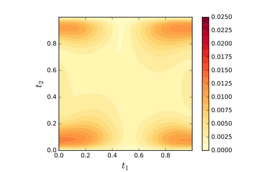 Figure 10
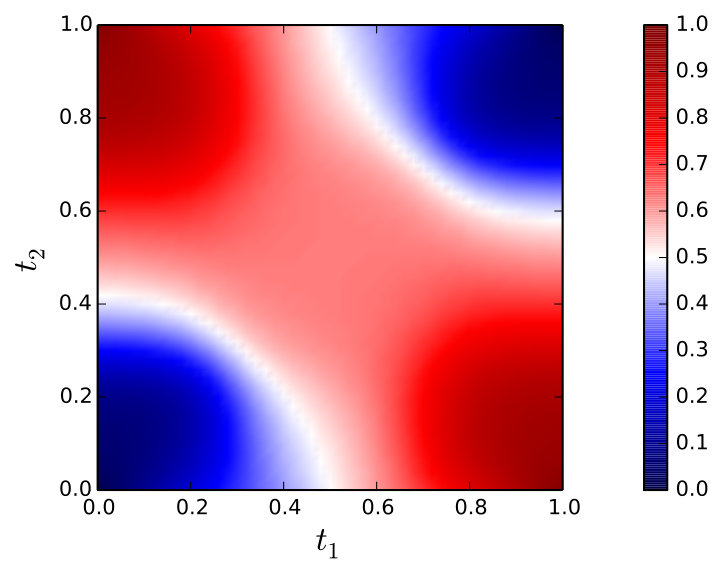 Figure 11
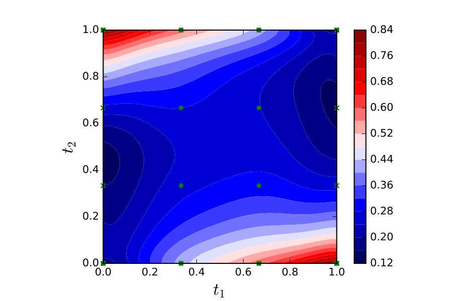 Figure 12
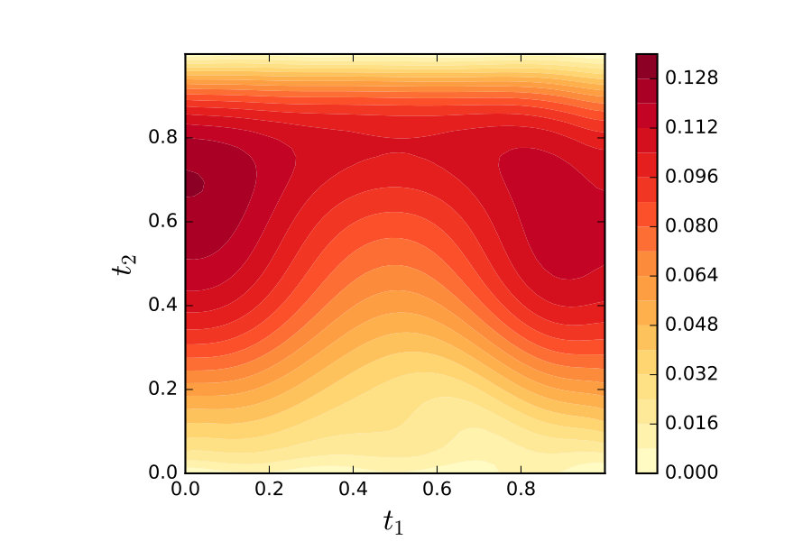 Figure 13
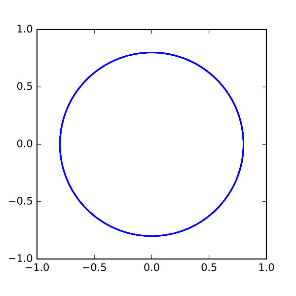 Figure 14
 Figure 15
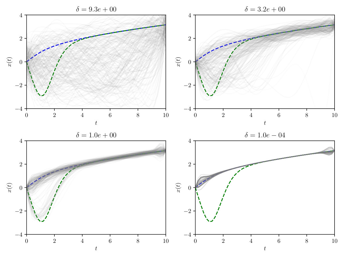 Figure 16
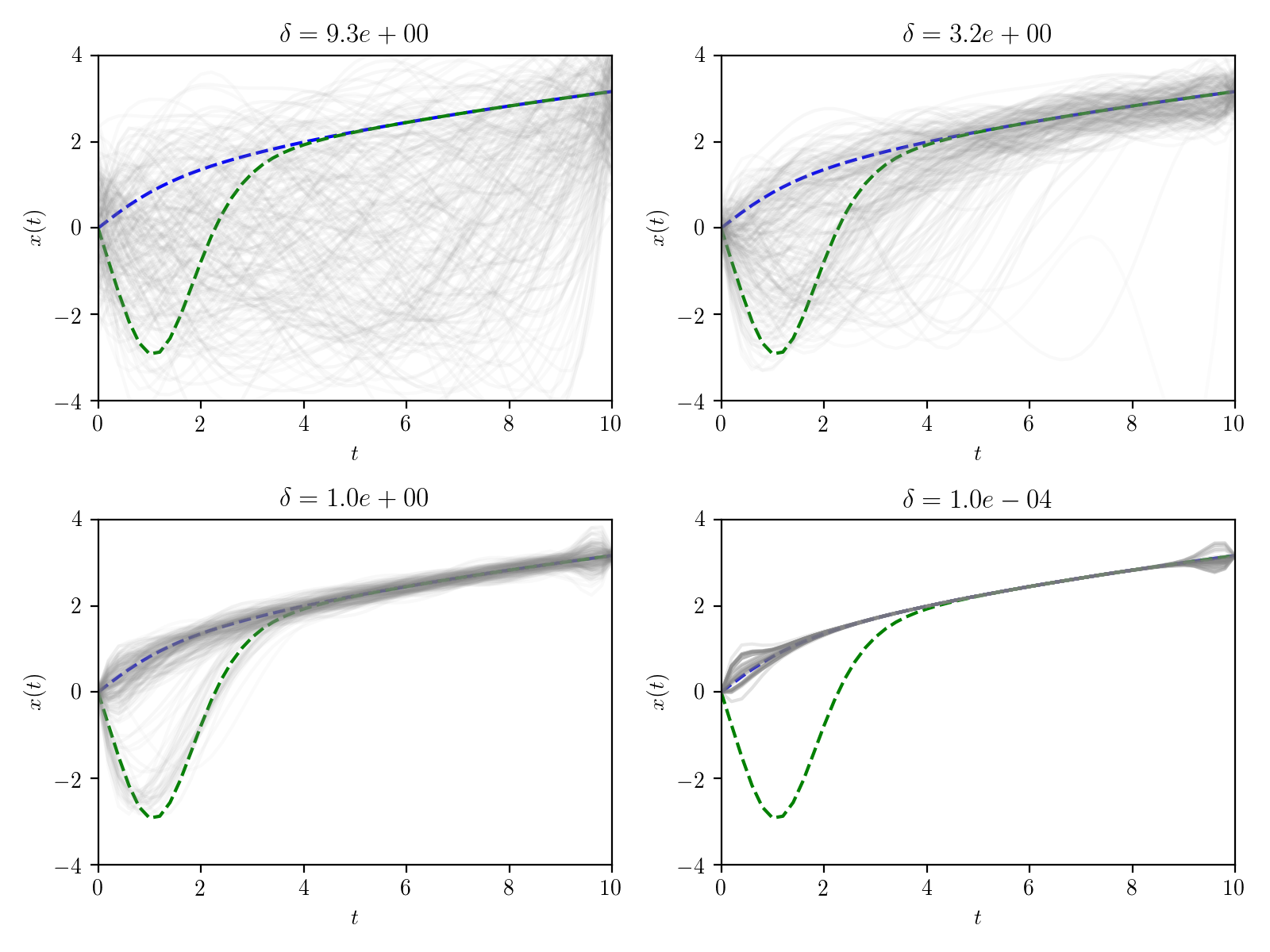 Figure 17
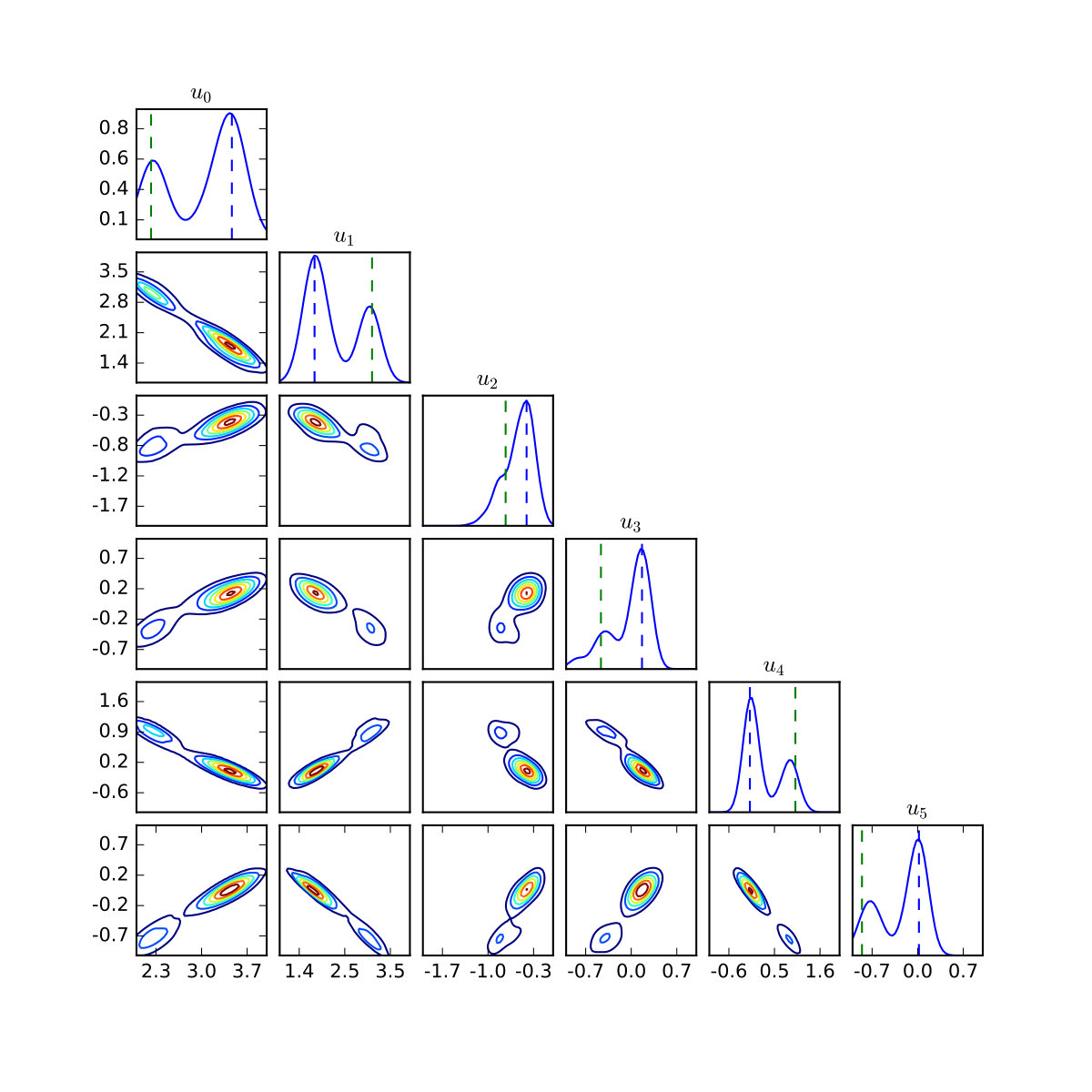 Figure 18
 Figure 19
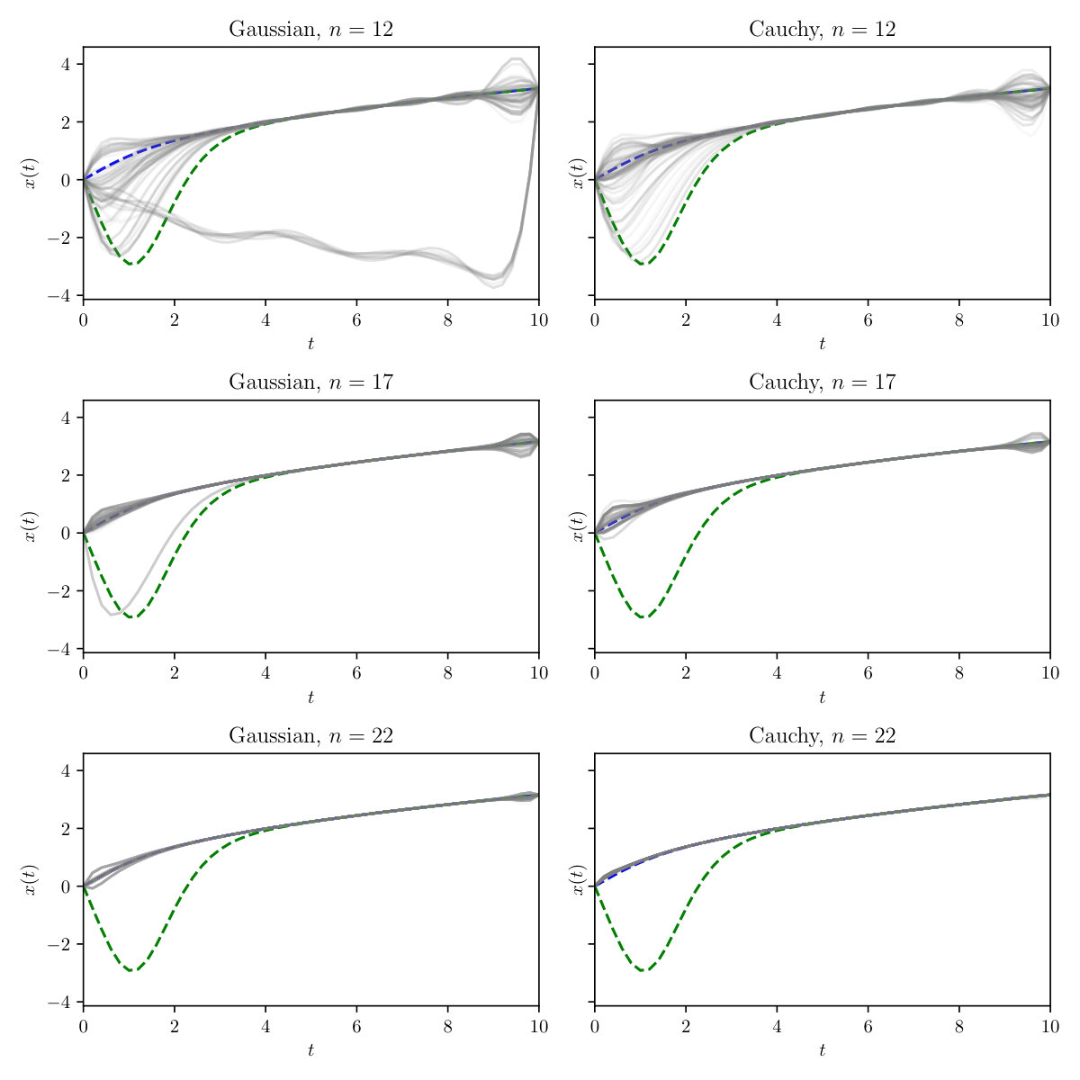 Figure 20
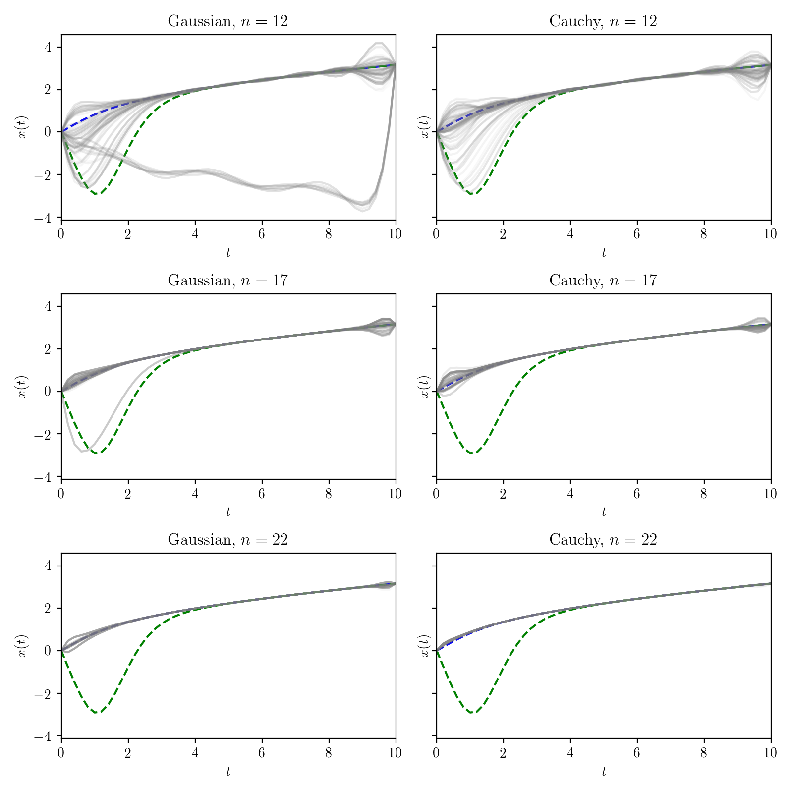 Figure 21
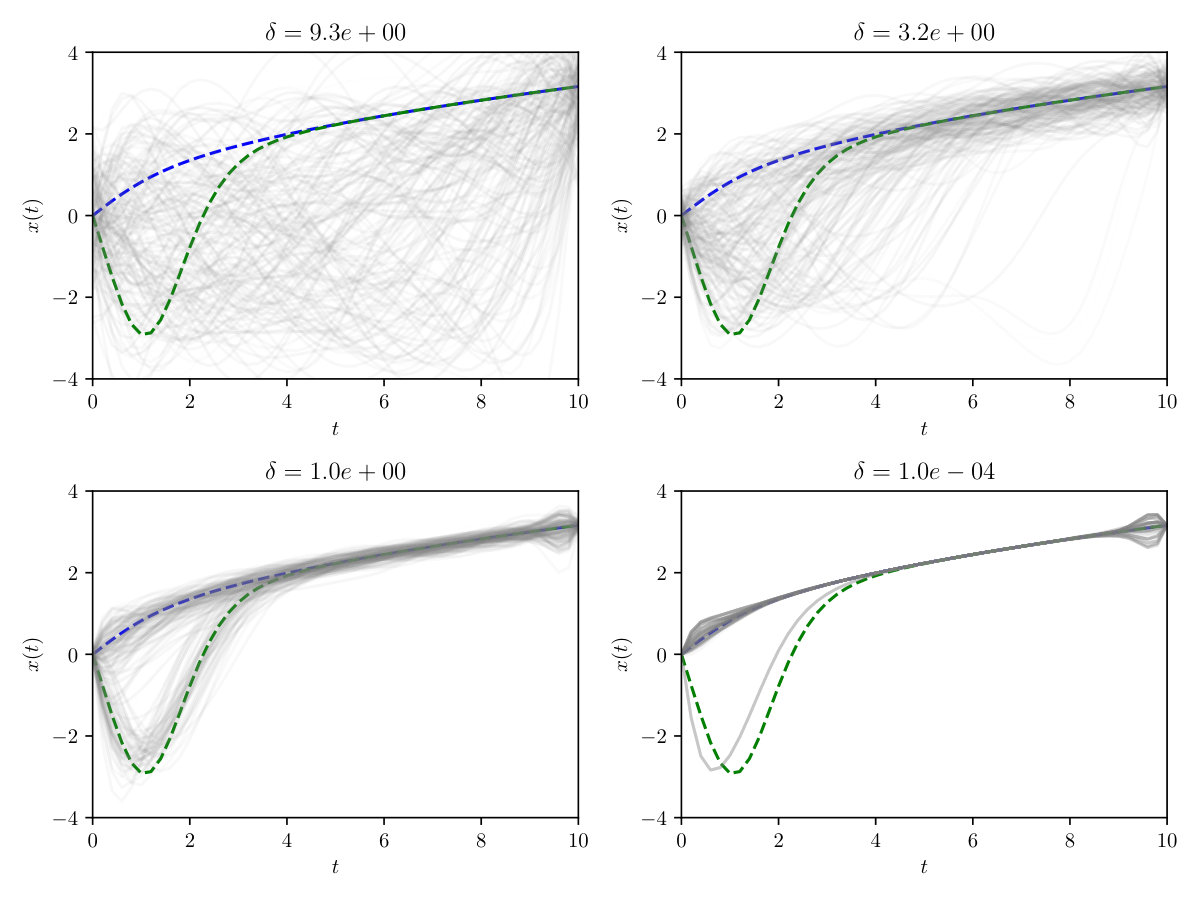 Figure 22
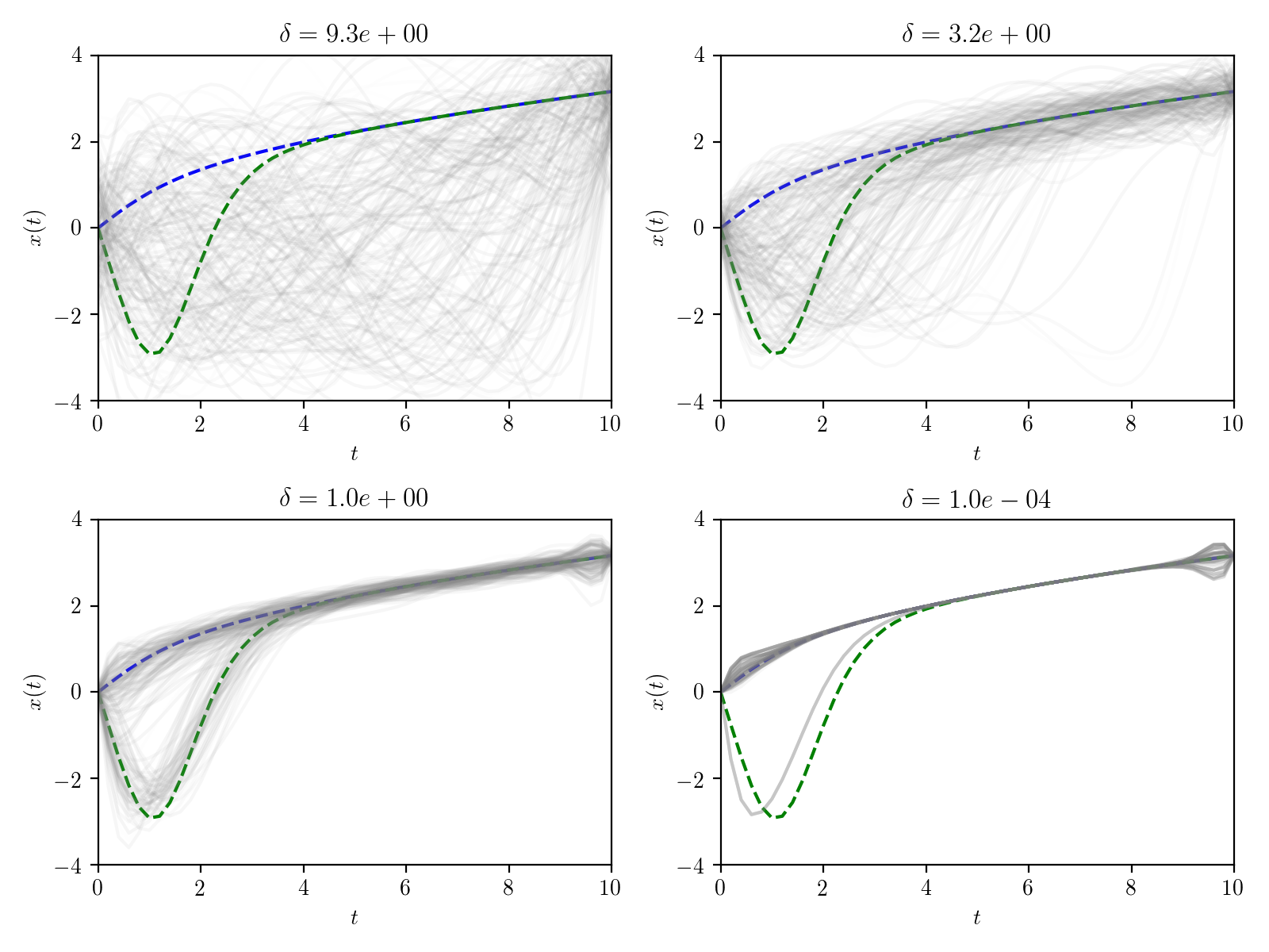 Figure 23
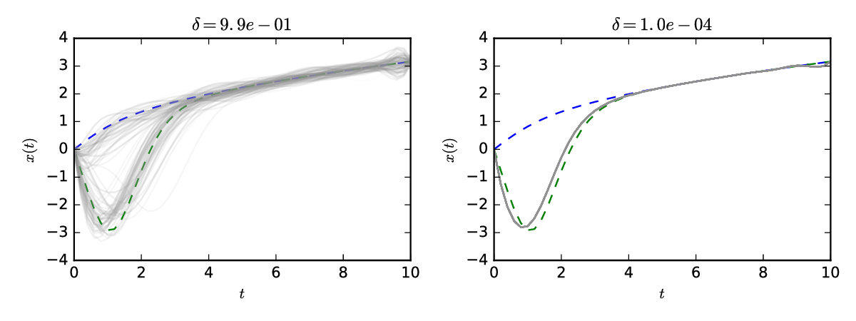 Figure 24
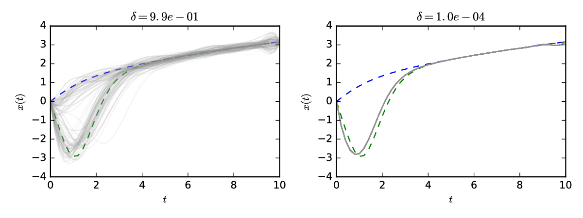 Figure 25
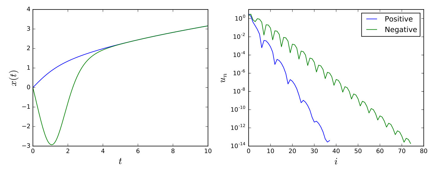 Figure 26
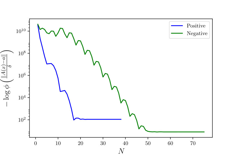 Figure 27
 Figure 28
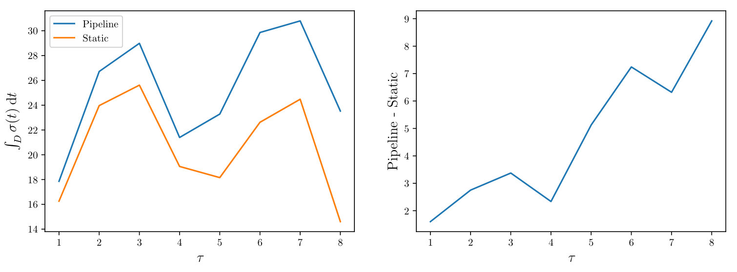 Figure 29
Peer Reviews
No public reviews on file for this paper yet. If you reviewed it on a platform where reviews are public (OpenReview, ICLR, NeurIPS, ICML), you can paste yours below so the community can read it here.
Videos
No videos yet. Explain this paper in a talk, walkthrough, or lecture? Add one.
Bayesian Probabilistic Numerical Methods
Jon Cockayne111University of Warwick, [email protected]
Chris Oates222Newcastle University and Alan Turing Institute, [email protected]
Tim Sullivan333Free University of Berlin and Zuse Institute Berlin, [email protected]
Mark Girolami444Imperial College London and Alan Turing Institute, [email protected]
Abstract
The emergent field of probabilistic numerics has thus far lacked clear statistical principals. This paper establishes Bayesian probabilistic numerical methods as those which can be cast as solutions to certain inverse problems within the Bayesian framework. This allows us to establish general conditions under which Bayesian probabilistic numerical methods are well-defined, encompassing both non-linear and non-Gaussian models. For general computation, a numerical approximation scheme is proposed and its asymptotic convergence established. The theoretical development is then extended to pipelines of computation, wherein probabilistic numerical methods are composed to solve more challenging numerical tasks. The contribution highlights an important research frontier at the interface of numerical analysis and uncertainty quantification, with a challenging industrial application presented.
1 Introduction
Numerical computation underpins almost all of modern scientific and industrial research and development. The impact of a finite computational budget is that problems whose solutions are high- or infinite-dimensional, such as the solution of differential equations, must be discretised in order to be solved. The result is an approximation to the object of interest. The declining rate of processor improvement as physical limits are reached is in contrast to the surge in complexity of modern inference problems, and as a result the error incurred by discretisation is attracting increased interest (e.g. Capistrán et al., 2016).
The situation is epitomised in modern climate models, where use of single-precision arithmetic has been explored to permit finer temporal resolution. However, when computing in single-precision, a detailed time discretisation can increase total error, due to the increased number of single precision computations, and in practice some form of ad-hoc trade-off is sought (Harvey and Verseghy, 2015). It has been argued that statistical considerations can permit more principled error control strategies for such models (Hennig et al., 2015).
Numerical methods are designed to mitigate discretisation errors of all forms (Press et al., 2007). Nonetheless, the introduction of error is unavoidable and it is the role of the numerical analyst to provide control of this error (Oberkampf and Roy, 2013). The central theoretical results of numerical analysis have in general not been obtained through statistical considerations. More recently, the connection of discretisation error to statistics was noted as far back as Henrici (1963); Hull and Swenson (1966), who argued that discretisation error can be modelled using a series of independent random perturbations to standard numerical methods. However, numerical analysts have cast doubt on this approach, since discretisation error can be highly structured; see Kahan (1996) and Higham (2002, Section 2.8). To address these objections, the field of probabilistic numerics has emerged with the aim to properly quantify the uncertainty introduced through discretisation in numerical methods.
The foundations of probabilistic numerics were laid in the 1970s and 1980s, where an important shift in emphasis occurred from the descriptive statistical models of the 1960s to the use of formal inference modalities that generalise across classes of numerical tasks. In a remarkable series of papers, Larkin (1969, 1970, 1972); Kuelbs et al. (1972); Larkin (1974, 1979a, 1979b), Mike Larkin presented now classical results in probabilistic numerics, in particular establishing the correspondence between Gaussian measures on Hilbert spaces and optimal numerical methods. Re-discovered and re-emphasised on a number of occasions, the role for statisticians in this new outlook was clearly captured in Kadane and Wasilkowski (1985):
Statistics can be thought of as a set of tools used in making decisions and inferences in the face of uncertainty. Algorithms typically operate in such an environment. Perhaps then, statisticians might join the teams of scholars addressing algorithmic issues.
The 1980s culminated in development of Bayesian optimisation methods (Mockus, 1989; Törn and Žilinskas, 1989), as well as the relation of smoothing splines to Bayesian estimation (Kimeldorf and Wahba, 1970b; Diaconis and Freedman, 1983).
The modern notion of a probabilistic numerical method (henceforth PNM) was described in Hennig et al. (2015); these are algorithms whose output is a distribution over an unknown, deterministic quantity of interest, such as the numerical value of an integral. Recent research in this field includes PNMs for numerical linear algebra (Hennig, 2015; Bartels and Hennig, 2016), numerical solution of ordinary differential equations (ODEs; Schober et al., 2014; Kersting and Hennig, 2016; Schober et al., 2016; Conrad et al., 2016; Chkrebtii et al., 2016), numerical solution of partial differential equations (PDEs; Owhadi, 2015; Cockayne et al., 2016; Conrad et al., 2016) and numerical integration (O’Hagan, 1991; Briol et al., 2016).
Open Problems
Despite numerous recent successes and achievements, there is currently no general statistical foundation for PNMs, due to the infinite-dimensional nature of the problems being solved. For instance, at present it is not clear under what conditions a PNM is well-defined, except for in the standard conjugate Gaussian framework considered in (Larkin, 1972). This limits the extent to which domain-specific knowledge, such as boundedness of an integrand or monotonicity of a solution to a differential equation, can be encoded in PNMs. In contrast, classical numerical methods often exploit such information to achieve substantial reduction in discretisation error. For instance, finite element methods for solution of PDEs proceed based on a mesh that is designed to be more refined in areas of the domain where greater variation of the solution is anticipated (Strang and Fix, 1973).
Furthermore, although PNMs have been proposed for many standard numerical tasks (see Section 2.6.1), the lack of common theoretical foundations makes comparison of these methods difficult. Again taking PDEs as an example, Cockayne et al. (2016) placed a probability distribution on the unknown solution of the PDE, whereas Conrad et al. (2016) placed a probability distribution on the unknown discretisation error of a numerical method. The uncertainty modelled in each case is fundamentally different, but at present there is no framework in which to articulate the relationship between the two approaches. Furthermore, though PNMs are often reported as being “Bayesian” there is no clear definition of what this ought to entail.
A more profound consequence of the lack of common foundation occurs when we seek to compose multiple PNMs. For example, multi-physics cardiac models involve coupled ODEs and PDEs which must each be discretised and approximately solved to estimate a clinical quantity of interest (Niederer et al., 2011). The composition of successive discretisations leads to non-trivial error propagation and accumulation that could be quantified, in a statistical sense, with PNMs. However, proper composition of multiple PNMs for solutions of ODEs and PDEs requires that these PNMs share common statistical foundations that ensure coherence of the overall statistical output. These foundations remain to be established.
Contributions
The main contribution of this paper is to establish rigorous foundations for PNMs:
The first contribution is to argue for an explicit definition of a “Bayesian” PNM. Our framework generalises the seminal work of Larkin (1972) and builds on the modern and popular mathematical framework of Stuart (2010). This illuminates subtle distinctions among existing methods and clarifies the sense in which non-Bayesian methods are approximations to Bayesian PNMs.
The second contribution is to establish when PNMs are well-defined outside of the conjugate Gaussian context. For exploration of non-linear, non-Gaussian models, a numerical approximation scheme is developed and shown to asymptotically approach the posterior distribution of interest. Our aim here is not to develop new or more computationally efficient PNMs, but to understand when such development can be well-defined.
The third contribution is to discuss pipelines of composed PNMs. This is a critical area of development for probabilistic numerics; in isolation, the error of a numerical method can often be studied and understood, but when composed into a pipeline the resulting error structure may be non-trivial and its analysis becomes more difficult. The real power of probabilistic numerics lies in its application to pipelines of numerical methods, where the probabilistic formulation permits analysis of variance (ANOVA) to understand the contribution of each discretisation to the overall numerical error. This paper introduces conditions under which a composition of PNMs can be considered to provide meaningful output, so that ANOVA can be justified.
Structure of the Paper
In Section 2 we argue for an explicit definition of Bayesian PNM and establish when such methods are well-defined. Section 3 establishes connections to other related fields, in particular with relation to evaluating the performance of PNMs. In Section 4 we develop useful numerical approximations to the output of Bayesian PNMs. Section 5 develops the theory of composition for multiple PNMs. Finally, in Section 6 we present applications of the techniques discussed in this paper.
All proofs can be found in either the Appendix or the Electronic Supplement.
2 Probabilistic Numerical Methods
The aim of this section is to provide rigorous statistical foundations for PNMs.
2.1 Notation
For a measurable space , the shorthand will be used to denote the set of all distributions on . For we write when is absolutely continuous with respect to . The notation will be used to denote a Dirac measure on , so that . Let denote the indicator function of an event . For a measurable function and a distribution , we will on occasion use the notation and . The point-wise product of two functions and is denoted . For a function or operator , denotes the associated push-forward operator555Recall that, for measurable , the pushforward of a distribution is defined as for all . that acts on measures on the domain of . Let denote conditional independence. The subset is defined to consist of sequences for which is convergent. will be used to denote the set of continuous functions on .
2.2 Definition of a PNM
To first build intuition, consider numerical approximation of the Lebesgue integral
[TABLE]
for some integrable function , with respect to a measure on . Here we may directly interrogate the integrand at any , but unless is finite we cannot evaluate at all with a finite computational budget. Nonetheless, there are many algorithms for approximation of this integral based on information at some collection of locations .
To see the abstract structure of this problem, assume the state variable exists in a measurable space . Information about is provided through an information operator whose range is a measurable space . Thus, for the Lebesgue integration problem, the information operator is
[TABLE]
The space , in this case a space of functions, can be high- or infinite-dimensional, but the space of information is assumed to be finite-dimensional in accordance with our finite computational budget. In this paper we make explicit a quantity of interest (QoI) , defined by a map into a measurable space . This captures that itself may not be the object of interest for the numerical problem; for the Lebesgue integration illustration, the QoI is not itself but .
The standard approach to such computational problems is to construct an algorithm which, when applied, produces some approximation of based on the information , whose theoretical convergence order can be studied. A successful algorithm will often tailor the information operator to the QoI . For example, classical Gaussian cubature specifies sigma points at which the integrand must be evaluated, based on exact integration of certain polynomial test functions.
The probabilistic numerical approach, instead, begins with the introduction of a random variable on . The true state is fixed but unknown; the randomness is used an abstract device used to represent epistemic uncertainty about prior to evolution of the information operator (Hennig et al., 2015). This is now formalised:
Definition 2.1** (Belief Distribution).**
An element is a belief distribution666Two remarks are in order: First, we have avoided the use of “prior” as this abstract framework encompasses both Bayesian and non-Bayesian PNMs (to be defined). Second, the use of “belief” differs to the set-valued belief functions in Dempster–Shafer theory, which do not require that (Shafer, 1976). for if it carries the formal semantics of belief about the true, unknown state variable .
Thus we may consider to be the law of . The construction of an appropriate belief distribution for a specific numerical task is not the focus of this research and has been considered in detail in previous work; see the Electronic Supplement for an overview of this material. Rather we consider the problem of how one updates the belief distribution in response to the information obtained about the unknown . Generic approaches to update belief distributions, which generalise Bayesian inference beyond the unique update demanded in Bayes theorem, were formalised in Bissiri et al. (2016); de Carvalho et al. (2017).
Definition 2.2** (Probabilistic Numerical Method).**
Let , and be measurable spaces and let , and where and are measurable functions. The pair is called a probabilistic numerical method for estimation of a quantity of interest . The map is called an information operator, and the map is called a belief update operator.
The output of a PNM is a distribution . This holds the formal status of a belief distribution for the value of , based on both the initial belief about the value of and the information that are input to the PNM.
An objection sometimes raised to this construction is that itself is not random. We emphasise that this work does not propose that should be considered as such; the random variable is a formal statistical device used to represent epistemic uncertainty (Kadane, 2011; Lindley, 2014). Thus, there is no distinction from traditional statistics, in which represents a fixed but unknown parameter and encodes epistemic uncertainty about this parameter.
Before presenting specific instances of this general framework, we comment on the potential analogy between and the likelihood function, and between and Bayes’ theorem. Whilst intuitively correct, the mathematical developments in this paper are not well-suited to these terms; in Section 2.5 we show that Bayes formula is not well-defined, as the posterior distribution is not absolutely continuous with respect to the prior.
To strengthen intuition we now give specific examples of established PNMs:
Example 2.3** (Probabilistic Integration).**
Consider the numerical integration problem earlier discussed. Take , a separable Banach space of real-valued functions on , and the Borel -algebra for . The space is endowed with a Gaussian belief distribution . Given information , define to be the restriction of to those functions which interpolate at the points ; that is again Gaussian follows from linearity of the information operator (see Bogachev, 1998, for details). The QoI remains .
This problem was first considered by Larkin (1972). The belief update operator proposed therein, and later considered in Diaconis (1988); O’Hagan (1991) and others, was . Since Gaussians are closed under linear projection, the PNM output is a univariate Gaussian whose mean and variance can be expressed in closed-form for certain choices of Gaussian covariance function and reference measure on . Specifically, if has mean function and covariance function , then
[TABLE]
where are defined as , , is defined as and . This method was extensively studied in Briol et al. (2016), who provided a listing of combinations for which and possess a closed-form.
An interesting fact is that the mean of coincides with classical cubature rules for different choices of and (Diaconis, 1988; Särkkä et al., 2016). In Section 3 we will show that this is a typical feature of PNMs. The crucial distinction between PNMs and classical numerical methods is the distributional nature of , which carries the formal semantics of belief about the QoI. The full distribution was examined in Briol et al. (2016), who established contraction to the exact value of the integral under certain smoothness conditions on the Gaussian covariance function and on the integrand. See also Kanagawa et al. (2016); Karvonen and Särkkä (2017).
Example 2.4** (Probabilistic Meshless Method).**
As a canonical example of a PDE, take the following elliptic problem with Dirichlet boundary conditions
[TABLE]
where we assume and is a known coefficient. Let be a separable Banach space of appropriately differentiable real-valued functions and take to be the Borel -algebra for . In contrast to the first illustration, the QoI here is , as the goal is to make inferences about the solution of the PDE itself.
Such problems were considered in Cockayne et al. (2016) wherein was restricted to be a Gaussian distribution on . The information operator was constructed by choosing finite sets of locations and at which the system defined in Eq. (2.3) was evaluated, so that
[TABLE]
The belief update operator was chosen to be , where is the restriction of to those functions for which is satisfied. In the setting of a linear system of PDEs such as that in Eq. (2.3), the distribution is again Gaussian (Bogachev, 1998). Full details are provided in Cockayne et al. (2016).
As in the previous example, we note that the mean of coincides with the numerical solution to the PDE provided by a classical method (the symmetric collocation method; Fasshauer, 1999). The full distribution provides uncertainty quantification for the unknown exact solution and can again be shown to contract to the exact solution under certain smoothness conditions (Cockayne et al., 2016). This method was further analysed for a specific choice of covariance operator in the belief distribution , in an impressive contribution from Owhadi (2017).
2.2.1 Classical Numerical Methods
Standard numerical methods fit into the above framework, as can be seen by taking
[TABLE]
independent of the distribution , where a function gives the output of some classical numerical method for solving the problem of interest. Here maps to a Dirac measure centred on . Thus, information in is used to construct a point estimate for the QoI.
The formal language of probabilities is not used in classical numerical analysis to describe numerical error. However, in many cases the classical and probabilistic analyses are mathematically equivalent. For instance, there is an equivalence between the standard deviation of for probabilistic integration and the worst-case error for numerical cubature rules from numerical analysis (Novak and Woźniakowski, 2010). The explanation for this phenomenon will be given in Section 3.
2.3 Bayesian PNMs
Having defined a PNM, we now state the central definition of this paper, that is of a Bayesian PNM. Define to be the conditional distribution of the random variable , given the event . For now we assume that this can be defined without ambiguity and reserve a more technical treatment of conditional probabilities for Section 2.5.
In this work we followed Larkin (1972) and cast the problem of determining in Eq. (2.1) as a problem of Bayesian inversion, a framework now popular in applied mathematics and uncertainty quantification research (Stuart, 2010). However, in a standard Bayesian inverse problem the observed quantity is assumed to be corrupted with measurement error, which is described by a “likelihood”. This leads, under mild assumptions, to general versions of Bayes’ theorem (see Stuart, 2010, Section 2.2)
For PNM, however, the information is not corrupted with measurement error. As a result, the support of the likelihood is a null set under the prior, making the standard approaches to such problems, including Bayes’ theorem, ill-defined outside of the conjugate Gaussian case when unknowns are infinite-dimensional. This necessitates a new definition:
Definition 2.5** (Bayesian Probabilistic Numerical Method).**
A probabilistic numerical method is said to be Bayesian777The use of “Bayesian” contrasts with Bissiri et al. (2016), for whom all belief update operators represent Bayesian learning algorithms to some greater or lesser extent. An alternative term could be “lossless”, since all the information in is conditioned upon in . for a quantity of interest if, for all , the output
[TABLE]
That is, a PNM is Bayesian if the output of the PNM is the push-forward of the conditional distribution through . This definition is familiar from the examples in Section 2.2, which are both examples of Bayesian PNMs.
For Bayesian PNMs we adopt the traditional terminology in which is the prior for and the output the posterior for . Note that, for fixed and , the Bayesian choice of belief update operator (if it exists) is uniquely defined.
It is emphasised that the class of Bayesian PNMs is a subclass of all PNMs; examples of non-Bayesian PNMs are provided in Section 2.6.1. Our analysis is focussed on Bayesian PNMs due to their appealing Bayesian interpretation and ease of generalisation to pipelines of computation in Section 5. For non-Bayesian PNMs, careful definition and analysis of the belief update operator is necessary to enable proper interpretation of the uncertainty quantification being provided. In particular, the analysis of non-Bayesian PNMs may present considerable challenges in the context of computational pipelines, whereas for Bayesian PNMs this is shown in Section 5 to be straight-forward.
2.4 Model Evidence
A cornerstone of the Bayesian framework is the model evidence, or marginal likelihood (MacKay, 1992). Let be equipped with the Lebesgue reference measure , such that admits a density . Then the model evidence , based on the information that , can be used as the basis for Bayesian model comparison. In particular, two prior distributions , , can be compared through the Bayes factor
[TABLE]
where . Here the second expression is independent of the choice of reference measure and is thus valid for general . The model evidence has been explored in connection with the design of Bayesian PNM. For the integration and PDE examples 2.3 and 2.4, the model evidence has a closed form and was investigated in Briol et al. (2016); Cockayne et al. (2016). In Section 6 we investigate the model evidence in the context of non-linear ODEs and PDEs for which it must be approximated.
2.5 The Disintegration Theorem
The purpose of this section is to formalise and to determine conditions under which exists and is well-defined. From Definition 2.5, the output of a Bayesian PNM is . If exists, the pushforward exists as is assumed to be measurable; thus, in this section, we focus on the rigorous definition of .
Unlike many problems of Bayesian inversion, proceeding by an analogue of Bayes’ theorem is not possible. Let . Then we observe that, if it is measurable, may be a set of zero measure under . Standard techniques for infinite-dimensional Bayesian inversion rely on constructing a posterior distribution based on its Radon–Nikodým derivative with respect to the prior (Stuart, 2010). However, when no Radon–Nikodým derivative exists and we must turn to other approaches to establish when a Bayesian PNM is well-defined.
Conditioning on null sets is technical and was formalised in the celebrated construction of measure-theoretic probability by Kolmogorov (1933). The central challenge is to establish uniqueness of conditional probabilities. For this work we exploit the disintegration theorem to ensure our constructions are well-defined. The definition below is due to Dellacherie and Meyer (1978, p.78), and a statistical introduction to disintegration can be found in Chang and Pollard (1997).
Definition 2.6** (Disintegration).**
For , a collection is a disintegration of with respect to the (measurable) map if:
- 1
(Concentration:) for -almost all ;
and for each measurable it holds that
- 2
(Measurability:) is measurable; 2. 3
(Conditioning:) .
The concept of disintegration extends the usual concept of conditioning of random variables to the case where is a null set, in a way closely related to regular conditional distributions (Kolmogorov, 1933). Existence of disintegrations is guaranteed under general weak conditions:
Theorem 2.7** (Disintegration Theorem; Thm. 1 of Chang and Pollard (1997)).**
Let be a metric space, be the Borel -algebra and be Radon. Let be countably generated and contain all singletons for . Then there exists a disintegration of with respect to . Moreover, if is another such disintegration, then is a null set.
The requirement that is Radon is weak and is implied when is a Radon space, which encompasses, for example, separable complete metric spaces. The requirement that is countably generated is also weak and includes the standard case where with the Borel -algebra. From Theorem 2.7 it follows that exists and is essentially unique for all of the examples considered in this paper. Thus, under mild conditions, we have established that Bayesian PNMs are well-defined, in that an essentially unique disintegration exists. It is noted that a variational definition of has been posited as an alternative approach, for when the existence of a disintegration is difficult to establish (p3 of Garcia Trillos and Sanz-Alonso, 2017).
2.6 Prior Construction
The Gaussian distribution is popular as a prior in the PNM literature for its tractability, both in the fact that finite-dimensional distributions take a closed-form and that an explicit conditioning formula exists. More general priors, such as Besov priors (Dashti et al., 2012) and Cauchy priors (Sullivan, 2016) are less easily accessed. In this section we summarise a common construction for these prior distributions, designed to ensure that a disintegration will exist.
Let denote an orthogonal Schauder basis for , assumed to be a separable Banach space in this section. Then any can be represented through an expansion
[TABLE]
for some fixed element and a sequence . Construction of measures is then reduced to construction of almost-surely convergent measures on and studying the pushforward of such measures into . In particular, this will ensure that is Radon (as is a separable complete metric space), a key requirement for existence of a disintegration .
To this end it is common to split into a stochastic and deterministic component; let represent an i.i.d sequence of random variables, and for some . Then with , for the prior distribution to be well-posed we require that almost-surely . Different choices of give rise to different distributions on . For instance, , is termed a uniform prior and gives a Gaussian prior, where determines the regularity of the covariance operator (Bogachev, 1998). The choice of gives a Cauchy prior in the sense of Sullivan (2016); here we require for a separable Banach space, or for when is a Hilbert space.
A range of prior specifications will be explored in Section 6, including non-Gaussian prior distributions for numerical solution of nonlinear ODEs.
2.6.1 Dichotomy of Existing PNMs
This section concludes with an overview of existing PNMs with respect to our definition of a Bayesian PNM. This serves to clarify some subtle distinctions in existing literature, as well as to highlight the generality of our framework. To maintain brevity we have summarised our findings in Table LABEL:table:comparison.
3 Decision-Theoretic Treatment
Next we assess the performance of PNMs from a decision-theoretic perspective (Berger, 1985) and explore connections to average-case analysis of classical numerical methods (Ritter, 2000). Note that the treatment here is agnostic to whether the PNM in question is Bayesian, and also encompasses classical numerical methods. Throughout, the existence of a disintegration will be assumed.
3.1 Loss and Risk
Consider a generic loss function where describes the loss incurred when the true QoI is estimated with . Integrability of is assumed.
The belief update operator returns a distribution over which can be cast as a randomised decision rule for estimation of . For randomised decision rules, the risk function is defined as
[TABLE]
The average risk of the PNM with respect to is defined as
[TABLE]
Here a state is drawn at random and the risk of the PNM output is computed. We follow the convention of terming the Bayes risk of the PNM, though the usual objection that a frequentist expectation enters into the definition of the Bayes risk could be raised.
Next, we consider a sequence of information operators indexed such that is -dimensional (i.e. pieces of information are provided about ).
Definition 3.1** (Contraction).**
A sequence of PNMs is said to contract at a rate under a belief distribution if .
This definition allows for comparison of classical and probabilistic numerical methods (Kadane and Wasilkowski, 1983; Diaconis, 1988). In each case an important goal is to determine methods that contract as quickly as possible for a given distribution that defines the Bayes risk. This is the approach taken in average-case analysis (ACA; Ritter, 2000) and will be discussed in Section 3.4. For Examples 2.3 and 2.4 of Bayesian PNMs, Briol et al. (2016) and Cockayne et al. (2016) established rates of contraction for particular prior distributions ; we refer the reader to those papers for details.
3.2 Bayes Decision Rules
A (possibly randomised) decision rule is said to be a Bayes rule if it achieves the minimum Bayes risk among all decision rules. In the context of (not necessarily Bayesian) PNMs, let and let
[TABLE]
That is, for fixed , is the set of all belief update operators that achieve minimum Bayes risk.
This raises the natural question of which belief update operators yield Bayes rules. Although the definition of a Bayes rule applies generically to both probabilistic and deterministic numerical methods, it can be shown888The proof is included in the Electronic Supplement. that if is non-empty, then there exists a which takes the form of a classical numerical method, as expressed in Eq. (2.4). Thus in general, Bayesian PNMs do not constitute Bayes rules, as the extra uncertainty inflates the Bayes risk, so that such methods are not optimal.
Nonetheless, there is a natural connection between Bayesian PNMs and Bayes rules, as exposed in Kadane and Wasilkowski (1983):
Theorem 3.2**.**
Let be a Bayesian probabilistic numerical method for the QoI . Let be an inner-product space and let the loss function have the form , where is the norm induced by the inner product. Then the decision rule that returns the mean of the distribution is a Bayes rule for estimation of .
This well-known fact from Bayesian decision theory999This is the fact that the Bayes act is the posterior mean under squared-error loss (Berger, 1985). is interesting in light of recent research in constructing PNMs whose mean functions correspond to classical numerical methods (Schober et al., 2014; Hennig, 2015; Särkkä et al., 2016; Teymur et al., 2016; Schober et al., 2016). Theorem 3.2 explains the results in Examples 2.3 and 2.4, in which both instances of Bayesian PNMs were demonstrated to be centred on an established classical method.
3.3 Optimal Information
The previous section considered selection of the belief update operator , but not of the information operator . The choice of determines the Bayes risk for a PNM, which leads to a problem of experimental design to minimise that risk.
The theoretical study of optimal information is the focus of the information complexity literature (Traub et al., 1988; Novak and Woźniakowski, 2010), while other fields such as quasi-Monte Carlo (QMC, Dick and Pillichshammer, 2010) attempt to develop asymptotically optimal information operators for specific numerical tasks, such as the choice of evaluation points for numerical approximation of integrals in the case of QMC. Here we characterise optimal information for Bayesian PNMs.
Consider the choice of from a fixed subset of the set of all possible information operators. To build intuition, for the task of numerical integration, could represent all possible choices of locations where the integrand is evaluated. For Bayesian PNM, one can ask for optimal information:
[TABLE]
where we have made explicit the fact that the optimal information depends on the choice of prior . Next we characterise , while an explicit example of optimal information for a Bayesian PNM is detailed in Example 3.4.
3.4 Connection to Average Case Analysis
The decision theoretic framework in Section 3.1 is closely related to average-case analysis (ACA) of classical numerical methods (Ritter, 2000). In ACA the performance of a classical numerical method is studied in terms of the Bayes risk given in Eq. (3.1), for the PNM with belief operator as in Eq. (2.4). ACA is concerned with the study of optimal information:
[TABLE]
In general there is no reason to expect and to coincide, since Bayesian PNM are not Bayes rules101010The distribution will in general not be supported on the set of Bayes acts.. Indeed, an explicit example where is presented in Appendix S3. However, we can establish sufficient conditions under which optimal information for a Bayesian PNM is the same as optimal information for ACA:
Theorem 3.3**.**
Let be an inner product space and the loss function have the form where is the norm induced by the inner product. Then the optimal information for a Bayesian PNM and for ACA are identical.
It is emphasised that this result is not a trivial consequence of the correspondance between Bayes rules and worst case optimal methods, as exposed in Kadane and Wasilkowski (1983). To the best of our knowledge, information-based complexity research has studied but not .
Theorem 3.3 establishes that, for the squared norm loss, we can extract results on optimal average case information from the ACA literature and use them to construct optimal Bayesian PNMs. An example is provided next.
Example 3.4** (Optimal Information for Probabilistic Integration).**
To illustrate optimal information for Bayesian PNMs, we revisit the first worked example of ACA, due to Sul*′*din (1959, 1960). Set and take the belief distribution to be induced from the Weiner process on , i.e. a Gaussian process with mean [math] and covariance function . Our QoI is and the loss function is .
Consider standard information for fixed knots . Our aim is to determine knots that represent optimal information for a Bayesian PNM with respect to and .
Motivated by Theorem 3.3 we first solve the optimal information problem for ACA and then derive the associated PNM. It will be sufficient to restrict attention to linear methods with . This allows a closed-form expression for the average error:
[TABLE]
Standard calculus can be used to minimise Eq. (3.2) over both the weights and the locations ; the full calculation can be found in Chapter 2, Section 3.3 of Ritter (2000). The result is an ACA optimal method
[TABLE]
which is recognised as the trapezium rule with equally spaced knots. The associated contraction rate is (Lee and Wasilkowski, 1986).
From Theorem 3.3 we have that ACA optimal information is also optimal information for the Bayesian PNM. Thus the optimal Bayesian PNM for the belief distribution is uniquely determined:
[TABLE]
Note how the PNM is centred on the ACA optimal method. However the PNM itself is not a Bayes rule; it in fact carries twice the Bayes risk as the ACA method.
This illustration can be generalised. It is known that for induced from the Weiner process on , a linear functional and a loss function that is convex and symmetric, equi-spaced evaluation points are essentially optimal information, the Bayes rule is the natural spline of degree , and the contraction rate is essentially ; see Lee and Wasilkowski (1986) for a complete treatment.
This completes our performance assessment for PNMs; next we turn to computational matters.
4 Numerical Disintegration
In this section we discuss algorithms to access the output from a Bayesian PNM. The approach considered in this paper is to form an explicit approximation to that can be sampled. The construction of a sampling scheme can exploit sophisticated Monte Carlo methods and allow probing at a computational cost that is de-coupled from the potentially substantial cost of obtaining the information itself.
The construction of an approximation to is non-trivial on a technical level. As shown in Section 2.5, under weak conditions on the space and the operator , the disintegration is well-defined for -almost all . The approach considered in this work is based on sampling from an approximate distribution which converges in an appropriate sense to in the limit. This follows in a similar spirit to Ackerman et al. (2017).
4.1 Sequential Approximation of a Disintegration
Suppose that is an open subset of and that the distribution , admits a continuous and positive density with respect to Lebesgue measure on . Further endow with the structure of a Hilbert space, with norm .
Let denote a decreasing function, to be specified, that is continuous at [math], with and . Consider
[TABLE]
where the normalisation constant
[TABLE]
is non-zero since is bounded away from 0 on a neighbourhood of and is bounded away from 0 on a sufficiently small interval . Our aim is to approximate with for small bandwidth parameter . The construction, which can be considered a mathematical generalisation of approximate Bayesian computation (Del Moral et al., 2012), ensures that . The role of is to admit states for which is close to but not necessarily equal. It is assumed to be sufficiently regular:
Assumption 4.1**.**
There exists such that .
To discuss the convergence of to we must first select a metric on . Let be a normed space of (measurable) functions with norm . For measures , define
[TABLE]
This formulation encompasses many common probability metrics such as the total variation distance and Wasserstein distance (Müller, 1997). However, not all spaces of functions lead to useful theory. In particular the total variation distance between and for will be one in general. Furthermore depending on the choice of , may be merely a pseudometric111111For a pseudometric, need not hold.. Sufficient conditions for weak convergence with respect to are now established:
Assumption 4.2**.**
The map is almost everywhere -Hölder continuous in , i.e.
[TABLE]
for some constant and for almost all .
Sufficient conditions for Assumption 4.2 are discussed in Ackerman et al. (2017), but are somewhat technical.
Theorem 4.3**.**
Let . Then, for sufficiently small,
[TABLE]
for almost all .
This result justifies the approximation of by when the QoI can be well-approximated by integrals with respect to . This result is stronger than that of earlier work, such as Pfanzagl (1979), in that it holds for infinite-dimensional , though it also relies upon the stronger Hölder continuity assumption.
The specific form for is not fundamental, but can impact upon rate constants. For the choice we have , which can be bounded independent of the dimension of . On the other hand, for it can be shown that, for ,
[TABLE]
so that the constant might not be bounded. In general this necessitates effective Monte Carlo methods that are able to sample from the regime where can be extremely small, in order to control the overall approximation error.
4.2 Computation for Series Priors
The series representation of in Eq. (2.6) of Section 2.6 is infinite-dimensional and thus cannot, in general, be instantiated. To this end, define and define the associated projection operator as
[TABLE]
A natural approach is to compute with the modified information operator instead of . This has the effect of updating the distribution of the first coefficients and leaving the tail unchanged, to produce an output . Then computation performed in the Bayesian update step is finite-dimensional, whilst instantiation of the posterior itself remains infinite-dimensional. A “likelihood-informed” choice of basis in such problems was considered in Cui et al. (2016).
Inspired by this approach, we next considered convergence of the output to in the limit . In this section it is additionally required that be everywhere continuous with . Let , so that is a continuous bijection of to itself. The following are also assumed:
Assumption 4.4**.**
For each , it holds that for some constant and all .
Assumption 4.5**.**
for all , where is measurable and satisfies and vanishes as is increased.
Assumption 4.6**.**
.
Assumption 4.7**.**
for some constant and all .
Assumption 4.4 holds for the case with constant . Assumption 4.5 is standard in the inverse problem literature; for instance it is shown to hold for certain series priors in Theorem 3.4 of Cotter et al. (2010). Assumption 4.6 is, in essence, a compactness assumption, in that it is implied by compactness of the state space when is linear. In this sense it is a strong assumption; however it can be enforced in our experiments, where is unbounded, through a threshold map
[TABLE]
where is a large pre-defined constant. Assumption 4.7 places a restriction on the probability metric in which our result is stated.
The following theorem has its proof in the Electronic Supplement:
Theorem 4.8**.**
For some constant , dependent on , it holds that .
An immediate consequence of Theorems 4.3 and 4.8 is that the total approximation error can be bounded by applying the triangle inequality:
[TABLE]
In particular, we have convergence of to in the limit provided that the number of basis functions satisfies .
The approximate posterior analysed above can be sampled when is Gaussian, since the first coefficients can be handled with MCMC and the tail , being Gaussian, can be sampled. However, when is non-Gaussian the tail is not recognised in a form that can be sampled. For the experiments in Section 6, in which both Gaussian and non-Gaussian priors are considered, the series in Eq. (2.6) was truncated at level , with the resultant prior denoted . The associated posterior was then entirely supported on the finite-dimensional subspace ; this is mathematically equivalent to working with the projected output . Analysis of prior truncation, as opposed to modification of the information operator just reported, is known to be difficult. Indeed, while converges to weakly, it does not do so in total variation, and this deficiency generally transfers to the associated posteriors. In general the impact of prior perturbation is a subtle topic — see e.g. Owhadi et al. (2015) and the references therein — and we therefore defer theoretical analysis of this approximation to future work.
4.3 Monte Carlo Methods for Numerical Disintegration
The previous sections established a sequence of well-defined distributions (or for non-Gaussian models) which converge (in a specific weak sense) to the exact disintegration . From construction, and this is sufficient to allow standard Monte Carlo methods to be used. The construction of Monte Carlo methods is de-coupled from the core material in the main text and the main methodological considerations are well-documented (e.g. Girolami and Calderhead, 2011).
For the experiments reported in subsequent sections two approaches were explored; a Sequential Monte Carlo (SMC) method (Doucet et al., 2001) and a parallel tempering method (Geyer, 1991). This provided a transparent sampling scheme, whose non-asymptotic approximation error can be theoretically understood. In particular, they provide robust estimators of model evidence that can be used for Bayesian model comparison. Full details of the Monte-Carlo methods used for this work, along with associated theoretical analysis for the SMC method, are contained in Section S4.1 of the Electronic Supplement.
5 Computational Pipelines and PNM
The last theoretical development in this paper concerns composition of several PNMs. Most analysis of numerical methods focuses on the error incurred by an individual method. However, real-world computational procedures typically rely on the composition of several numerical methods. The manner in which accumulated discretisation error affects computational output may be highly non-trivial (Roy, 2010; Anderson, 2011; Babuška and Söderlind, 2016). An extreme example occurs when one of the numerical methods in a pipeline is charged with integration of a chaotic dynamical system (Strogatz, 2014).
In recent work, Chkrebtii et al. (2016), Conrad et al. (2016) and Cockayne et al. (2016) each used PNMs within a broader statistical procedure to estimate unknown parameters in systems of ODEs and PDEs. The probabilistic description of discretisation error was incorporated into the data-likelihood, resulting in posterior distributions for parameters with inflated uncertainty to properly account for the inferential impact of discretisation error. However, beyond these limited works, no examination of the composition of PNMs has been performed. In particular, the question of which PNMs can be composed, and when the output of such a composition is meaningful, has not been addressed. This is important; for instance, if the output of a composition of PNMs is to be used for analysis of variance to elucidate the main sources of discretisation error, then it is important that such output is meaningful.
This section defines a pipeline as an abstract graphical object that may be combined with a collection of compatible PNMs. It is proven that when compatible Bayesian PNMs are employed in the pipeline, the distributional output of the pipeline carries a Bayesian interpretation under an explicit conditional independence condition on the prior .
To build intuition, for the simple case where two Bayesian PNMs are composed in series, our results provide conditions for when, informally, the output corresponds to a single Bayesian procedure . To reduce the notational and technical burden, in this section we will not provide rigorous measure theoretic details; however we note that those details broadly follow the same pattern as in Section 2.5.
5.1 Computational Pipelines
To analyse pipelines of PNMs, we consider such methods , where each method is defined on a common121212This is without loss of generality, since can be taken as the union of all state spaces required by the individual methods. state space and targets a QoI . A pipeline will be represented as a directed graphical model, wherein the QoIs from parent methods constitute information operators for child methods. It may be that a method will take quantities from multiple parents as input. To allow for this, we suppose that the information operator can be decomposed into components such that and . Thus, each component can be thought of as the QoI output by one of the parents of the method .
Without loss of generality we designate the th QoI to be the principal QoI. That is, the purpose of the computational pipeline is to estimate . The case of multiple principal QoI is a simple extension not described herein. Nodes with no immediate children are called terminal nodes, while nodes with no immediate parents are called source nodes. We denote by the set of all source nodes.
Definition 5.1** (Pipeline).**
A pipeline is a directed acyclic graph defined as follows:
- •
Nodes are of two kinds: Information nodes are depicted by , and method nodes are depicted by .
- •
The graph is bipartite, so that edges connect a method node to an information node or vice-versa. That is, edges are of the form or .
- •
There are method nodes, each with a unique label in .
- •
The method node labelled has parents and one child. Its in-edges are assigned a unique label in .
- •
There is a unique terminal node and it is the child of method node . This represents the principal QoI .
Example 5.2** (Distributed Integration).**
Recall the numerical integration problem of Example 3.4 and, as a thought experiment, consider partitioning the domain of integration in order to distribute computation:
[TABLE]
To keep presentation simple we consider an integral over with equidistant knots . Let be a Bayesian PNM for estimating (a) and be a Bayesian PNM for estimating (b).
In terms of our notational convention, we divide the information operator into four components; , for . and contain the information unique to and . Specifically
[TABLE]
and contain the information that is shared between the two methods; that is . To complete the specification we need a third PNM for estimation of (c) which we denote and which combines the outputs of and by simply adding them together. Formally this has information operator where (a) and (b). Its belief update operator is given by:
[TABLE]
An intuitive graphical representation of this set-up is shown in Figure 1. The pipeline itself, which is identical to Figure 1 but with additional node and edge labels, is shown in Figure 2.
In general, the method node labelled is taken to represent the method . The in-edge to this node labelled is taken to represent the information provided by the relationship . Here can either be deterministic information provided to the pipeline, or statistical information derived from the output of another PNM. To make this formal and to “match the input-output spaces” we next define what it means for the collection of methods to be compatible with the pipeline . Informally, this describes the conditions that must be satisfied for method nodes in a pipeline to be able to connect to each other.
Definition 5.3** (Compatible).**
The collection of PNMs is compatible with the pipeline if the following two requirements are satisfied:
- (i)
(Method nodes which share an information node must have consistent information spaces and information operators.) For a motif
i$$j$$i^{\prime}$$j^{\prime}
we have that and . 2. (ii)
(The space for the output of a previous method must be consistent with the information space of the next method.) For a motif
i$$j$$j^{\prime}
we have that .
Note that we do not require the converse of (i) at this stage; that is, the same information can be represented by more than one node in the pipeline. This permits redundancy in the pipeline, in that information is not recycled. It will transpire that pipelines with such redundancy are non-Bayesian.
The role of the pipeline is to specify the order in which information, either deterministic of statistical, is propagated through the collection of PNMs. This is illustrated next:
Example 5.4** (Propagation of Information).**
For the pipeline in Figure 2, the propagation of information proceeds as follows::
The source nodes, representing are evaluated as . This represents all the information on that is provided. 2. 2.
The distributions
[TABLE]
are computed. 3. 3.
The push-forward distribution
[TABLE]
is computed.
Here is defined on the Cartesian product with independent components and . The notation refers to the push-forward of the function over its second argument. The distribution is the output of the pipeline and is a distribution over the principal QoI .
The procedure in Example 5.4 can be formalised, but to keep the presentation and notation succinct, we leave this implicit:
Definition 5.5** (Computation).**
For a collection of PNMs that are compatible with a pipeline , the computation is defined as the PNM with information operator and belief update operator that takes and as input and returns the distribution as its output , obtained through the procedure outlined in Example 5.4.
That is, the computation is a PNM for the principal QoI . Note that this definition includes a classical numerical work-flow just as a PNM encompasses a standard numerical method.
5.2 Bayesian Computational Pipelines
Noting that is itself a PNM, there is a natural definition for when such a computation can be called Bayesian:
Definition 5.6** (Bayesian Computation).**
Denote by the information and belief operators associated with the computation and let be a disintegration of with respect to the information operator . The computation is said to be Bayesian for the QoI if
[TABLE]
This is clearly an appealing property; the output of a Bayesian computation can be interpreted as a posterior distribution over the QoI given the prior and the information . Or, more informally, the “pipeline is lossless with information”. However, at face value it seems difficult to verify whether a given computation is Bayesian, since it depends on both the individual PNMs and the pipeline that combines them. Our next aim is to establish verifiable sufficient conditions, for which we require another definition:
Definition 5.7** (Dependence Graph).**
The dependence graph of a pipeline is the directed acyclic graph obtained by taking the pipeline , removing the method nodes and replacing all motifs with direct edges .
The dependency graph for Example 5.2 is shown in Figure 3.
For a computation , each of the distinct nodes in can be associated with a random variable where either for some , when the node is a source, or otherwise , for some . Randomness here is understood to be due to , so that the distribution of the is a function of . The convention used here is that the are indexed according to a topological ordering on , which has the properties that (i) the source nodes correspond to indices , and (ii) the final random variable is .
Definition 5.8** (Coherence).**
Consider a computation . Denote by the parent set of node in the dependence graph . Then we say that is coherent for the computation if the implied joint distribution of the random variables satisfies:
[TABLE]
for all .
Note that this is weaker than the Markov condition for directed acyclic graphs (see Lauritzen, 1991), since we do not insist that the variables represented by the source nodes are independent. It is emphasised that, for a given , the coherence condition can in general be checked and verified.
The following result provides sufficient and verifiable conditions which ensure that a computation composed of individual Bayesian PNMs is a Bayesian computation:
Theorem 5.9**.**
Let be Bayesian PNMs and let be coherent for the computation . Then it holds that the computation is Bayesian for the QoI .
Conversely, if non-Bayesian PNM are combined then the computation need not be Bayesian in general.
Example 5.10** (Example 5.2, continued).**
The random variables in this example are:
[TABLE]
From in Figure 3, coherence condition in Definition 5.8 requires that the non-trivial conditional independences and hold. Thus the distribution is coherent for the computation if and only if, for , the associated information variables satisfy and .
The distribution induced by the Weiner process on in Example 3.4 satisfies these conditions. Indeed, under the stochastic process is conditionally independent of its history given the current state . Thus for this choice of , from Theorem 5.9 we have that is Bayesian and parallel computation of and in Eq. (5.1) can be justified from a Bayesian statistical standpoint.
However, for the alternative of belief distributions induced by the Weiner process on , this condition is not satisfied and the computation is not Bayesian. To turn this into a Bayesian procedure for these alternative belief distributions it would be required that provides information about the derivatives for all orders .
5.3 Monte Carlo Methods for Probabilistic Computation
The most direct approach to access is to sample from each Bayesian PNM and treat the output samples as inputs to subsequent PNM. This is sometimes known as ancestral sampling in the Bayesian network literature (e.g. Paige and Wood, 2015), and is illustrated in the following example:
Example 5.11** (Ancestral Sampling for PNM).**
For Example 5.2, ancestral sampling proceeds as follows:
Draw initial samples
[TABLE] 2. 2.
Draw a final sample
[TABLE]
Then is a draw from .
Ancestral sampling requires that PNM outputs can be sampled. Such sampling methods were discussed in Section 4.3. For a more general approach, sequential Monte Carlo methods can be used to propagate a collection of particles through the pipeline , similar to work on SMC for general graphical models (Briers et al., 2005; Ihler and McAllester, 2009; Lienart et al., 2015; Lindsten et al., 2017; Paige and Wood, 2015).
6 Numerical Experiments
In this final section of the paper we present three numerical experiments. The first is a linear PDE, the second is a nonlinear ODE and the third is an application to a problem in industrial process monitoring, described by a pipeline of PNM. In each case we experiment with non-Gaussian belief distributions and, in doing so, go beyond previous work.
6.1 Poisson Equation
Our first illustration is an instance of the Poisson equation, a linear PDE with mixed Dirichlet-Neumann boundary conditions:
[TABLE]
A model solution to this system, generated with a finite-element method on a fine mesh, is shown in Figure 4.
As the spatial domain for this problem is two-dimensional, the basis used for specification of the belief distribution is more complex. Here tensor products of orthogonal polynomials have been used: , . The polynomials were chosen to be normalised Chebyshev polynomials of the first kind. Prior specification then follows the formulation given in Section 2.6, where the remaining parameters were chosen to be , and . The random variables were taken to be either Gaussian or Cauchy and the polynomial basis was truncated to terms, corresponding to a maximum polynomial degree of . For both priors the parameter was set to . Note that closed-form expressions are available for analysis under the Gaussian prior (Cockayne et al., 2016) but, to simplify interpretation of empirical results, were not exploited. Mathematical background on Cauchy priors can be found in Sullivan (2016).
The information operator was defined by a set of locations , , where either the interior condition or one of the boundary conditions was enforced. Denote by the set of interior points, the set of Dirichlet boundary points and the set of Neumann boundary points, where , and , with . Then, the information operator is given by the concatenation of the conditions defined above:
[TABLE]
[TABLE]
The Bayesian PNM output was approximated by numerical disintegration and sampled with a Monte Carlo method whose description is reserved for the Electronic Supplement. In Figure 5 the mean and pointwise standard-deviations of the posterior distributions are plotted for Gaussian and Cauchy priors with . There is little qualitative difference between the posterior distributions for the Gaussian and Cauchy priors. The mean functions match closely to the mean function from the model solution, as given in Figure 4. The posterior variance is lowest near to the Dirichlet boundaries where the solution is known, and peaks where the Neumann condition is imposed. This is to be expected, as evaluations of the Neumann boundary condition provide less information about the solution itself.
Next, the posterior distribution of the spectrum was investigated. In Figure 6 the posterior distribution over these coefficients is plotted and it is seen that the correlation structure between coefficients is non-trivial, c.f. the joint distribution between and .
Last, in Figure 7 convergence of the posterior distribution is plotted as the number of design points is varied, for . In each case a Gaussian prior was used. As expected, the standard deviation in the posterior distribution is seen to decrease as the number of design points is increased. At , the shape of the region of highest uncertainty changes markedly, with the most uncertain region lying between the Dirichlet boundary and the first evaluation points on the Neumann boundary. This is likely due to the fact that the number of evaluation points is approaching the size of the polynomial basis; when the number of points equals the size of the basis the system is completely determined for a linear model. Thus, we need in order for discretisation error to be quantified.
6.2 The Painlevé ODE
In this section a Bayesian PNM is developed to solve a nonlinear ODE based on Painlevé’s first transcendental
[TABLE]
To permit computation, the right-boundary condition was relaxed by truncating the domain to and using the modified condition .
Two distinct solutions are known, illustrated in Figure 8 (left). These model solutions were obtained using the deflation technique described in Farrell et al. (2015). The spectrum plot in Figure 8 (right) represents the coefficients obtained when each solution is represented over a basis of normalised Chebyshev polynomials. As those polynomials are orthonormal with respect to the -inner-product, the slower decay for the negative solution compared to the positive solution is equivalent to the negative solution having a larger -norm. This explains the preference that optimisation-based numerical solvers have for returning the positive solution in general, and also explains some of the results now presented.
Such systems for which multiple solutions exist have been studied before in the context of PNM, both in Chkrebtii et al. (2016) and in Cockayne et al. (2016). It was noted in both papers that existence of multiple solutions can present a substantial challenge to classical numerical methods.
To build a Bayesian PNM, a prior for this problem was defined by using a series expansion as in Eq. (2.6). The basis functions were where the were normalised Chebyshev polynomials of the first kind. Both Gaussian and Cauchy priors were considered by taking , where were taken to be either standard Gaussian or standard Cauchy and in in each case . In accordance with the exponential convergence rate for spectral methods when the solution to the system is a smooth function, the sequence of scale parameters was set to , where and . These values were chosen by inspection of the true spectra (obtained with Matlab’s “chebfun” package) to ensure that both solutions were in the support of the prior.
The information operator was defined by the choice of locations , , which determine the locations at which the posterior will be constrained. Analysis for several values of was performed. In each case , and the remaining were equally spaced on . To be explicit, the information operator was
[TABLE]
with the last two elements enforcing the boundary conditions. Thus our information was , which is dimensional.
The Bayesian PNM output was approximated via numerical disintegration with the first terms of the series representation used. This was sampled with Monte Carlo methods, the details of which are reserved for the Electronic Supplement.
Results for a selection of bandwidths , with , are shown in Figure 9. Note that a strong preference for the positive solution is expressed at the smallest , with mass around both solutions at larger . For the Gaussian prior, some mass remained around the negative solution at the smallest , while this was not so for the Cauchy prior. This reflects the fact that, for a collection of independent univariate Cauchy random variables, one element is likely to be significantly larger in magnitude than the others, which favours faster decay for the remaining elements.
Using the calculation described in Section S4.4, model evidence was computed for both the Gaussian and the Cauchy prior at . The Bayes factor for the Cauchy, compared to the Gaussian prior, was found to be , which constitutes strong evidence in favour of a Cauchy prior for this problem at the given level of discretisation.
In Figure 10 the posterior distributions for first six coefficients at and are plotted. Strong multimodality is clear, as well as skewed correlation structure between the coefficients. Illustration of such posteriors for smaller is difficult as the posteriors become extremely peaked.
Figure 11 displays convergence of the posterior distributions as is increased. Of particular interest is that for , the posterior distribution based on a Gaussian prior becomes trimodal. For each prior, the posterior mass settles on the positive solution to the system at . This is in accordance with the fact that this solution has smaller -norm. This perhaps reflects the fact that, while in the limiting case both solutions should have an equal likelihood, the curvature of the likelihood at each mode may differ. Prior truncation may also be influential; in Figure 12 the log-likelihood of the negative solution increases at a slower rate than that of the positive solution. Thus, while in the setting of an infinite prior series neither solution should be preferred, in practice truncation might bias one solution over the other. Lastly, it is clear that the parameters and may also have a significant effect on which solution is preferred. Further theoretical work will be required to understand many of the phenomena that we have just described.
Of particular interest is how a preference for the negative solution could be encoded into a PNM. Owing to the flexible specification the information operator, there is considerable choice in this matter. An elegant approach is the introduction of additional, inequality-based information
[TABLE]
Such information can be difficult to incorporate in standard numerical algorithms, but is of interest in many physical problems (Kinderlehrer and Stampacchia, 2000). For Bayesian PNM we can extend the information operator to include . Posterior distributions for the Gaussian prior at are shown in Figure 13. Note that posterior mass has settled close to the negative solution. This highlights the simplicity with which Bayesian PNMs can encode a preference for a particular solution when a multiplicity of solutions exist.
6.3 Application to Industrial Process Monitoring
This final application illustrates how statistical models for discretisation error can be propagated through a pipeline of computation to model how these errors are accumulated.
Hydrocyclones are machines used to separate solid particles from a liquid in which they are suspended, or two liquids of different densities, using centrifugal forces. High pressure fluid is injected into the top of a tank to create a vortex. The induced centrifugal force causes denser material to move to the wall of the tank while lighter material concentrates in the centre, where it can be extracted. They have widespread applications, including in areas such as environmental engineering and the petrochemical industry (Sripriya et al., 2007). An illustration of the operation is given in Figure 14.
To ensure the materials are well-separated the hydrocyclone must be moitored to allow adjustment of the input flow-rate. This is also important for safe operation, owing to the high pressures involved (Bradley, 2013). However, direct monitoring is impossible owing to the opaque walls of the equipment and the high interior pressure. For this purpose electrical impedance tomography (EIT) has been proposed to allow monitoring of the contents (Gutierrez et al., 2000).
EIT is a technique which allows recovery of an interior conductivity field based upon measurements of voltage obtained from applying a stimulating current on the boundary. It is suited to this problem, as the two materials in the hydrocyclone will generally be of different conductivities. In its simplified form due to Calderón (1980), EIT is described by a linear partial differential equation similar to that in Section 6.1, but with modified boundary conditions to incorporate the stimulating currents and measured voltages:
[TABLE]
where denotes the domain, modelling the hydrocyclone tank, indexes the stimulating electrodes, are the corresponding locations of the electrodes on , is the unknown conductivity field to be determined and denotes the derivative with respect to the outward pointing normal vector. The electrode is referred to as the reference electrode. The vector denotes the stimulation current pattern. Several stimulation patterns were considered, denoted , .
The experimental data described in West et al. (2005) were considered. In the experiment, a cylindrical perspex tank was used with a single ring of eight electrodes. Translation invariance in the vertical direction means that the contents are effectively a single 2D region and electrical conductivity can be modelled as a 2D field. At the start of the experiment, a mixing impeller was used to create a rotational flow. This was then removed and, after a few seconds, concentrated potassium chloride solution was carefully injected into the tap water initially filling the tank. Data, denoted , were collected at regular time intervals by application of several stimulation patterns .
To formulate the statistical problem, consider parameterising the conductivity field as , where is a temporal index while is the spatial coordinate and is the circular domain representing the perspex tank in the experiment. A log-Gaussian prior was placed over the conductivity field so that is a Gaussian process with separable covariance function where is a length-scale parameter representing the anticipated spatial variation of the conductivity field and is a parameter controlling the amplitude of the field. Here was fixed to , while . The problem of estimating based on data can be well-posed in the Bayesian framework (Dunlop and Stuart, 2016). Full details of this experiment can be found in the accompanying report Oates et al. (2017).
Our aim is to use a PNM to account for the effect of discretisation on inferences that are made on the conductivity field. For fixed , a Gaussian prior was posited for , with covariance where was fixed to . The associated Bayesian PNM, a probabilistic meshless method (PMM), was described in Example 2.4.
The statistical inference procedure is formulated in a pipeline of computations in Figure 15. It is assumed that the desired outcome is to monitor the contents of the tank while the current contents are being mixed. This suggests a particle filter approach where a PMM is employed to handle the intractable likelihood that involves the exact solution of a PDE. The distribution of given is denoted an the computation is Bayesian only if the particle approximation error due to the use of a particle filter is overlooked.
To briefly illustrate the method, Figure 16 presents posterior means for the field , for each post-injection time point . These are based on a particle approximation of size , with method nodes based upon a Bayesian PNM, as in Example 2.4, with design points. The high conductivity region representing the potassium chloride solution can be seen rotating through the domain in the frames after injection, with its conductivity reducing as it mixes with the water. The full posterior distribution over the conductivity field is inflated as a result of explicitly modelling the discretisation error; an extensive analysis of these results will be reported in the upcoming Oates et al. (2017).
In Figure 17, the integrated standard-deviation is shown for for both the “pipeline”, as described above, and a “static” approach in which no uncertainty was propagated. In this static approach a symmetric collocation PDE solver131313Recall that the PMM has a corresponding symmetric collocation solution to the PDE as its mean function. was used to solve the forward problem, and a separate Bayesian inversion problem was solved at each time point. The parameters of the symmetric collocation solver were identical to those used in the PMM. In the left panel we observe some structural periodicity, present in both the pipeline and the static approach. We speculate that this may be due to the rotation of the medium causing the area of high conductivity to periodically reach an area of the domain, relative to the 8 sensors, in which it is particularly easy to recover. With this periodicity subtracted in the right panel, there was a clear increase in posterior uncertainty in the pipeline compared to the static approach, which is depicted. Temporal regularisation would usually be expected to reduce uncertainty; thus, the fact that the overall uncertainty increased with , relative to the static formulation, demonstrates that we have quantified and propagated uncertainty due to successive discretisation of the PDE at each time point.
7 Discussion
This paper has established statistical foundations for PNMs and investigated the Bayesian case in detail. Through connection to Bayesian inverse problems (Stuart, 2010), we have established when Bayesian PNM can be well-defined and when the output can be considered meaningful. The presentation touched on several important issues and a brief discussion of the most salient points is now provided.
Bayesian vs Non-Bayesian PNMs
The decision to focus on Bayesian PNMs was motivated by the observation that the output of a pipeline of PNMs can only be guaranteed to admit a valid Bayesian interpretation if the constituent PNMs are each Bayesian and the prior distribution is coherent. Indeed, Theorem 5.9 demonstrated that prior coherence can be established at a local level, essentially via a local Markov condition, so that Bayesian PNMs provide a extensible modelling framework as required to solve more challenging numerical tasks. These results support a research strategy that focuses on Bayesian PNMs, so that error can be propagated in a manner that is meaningful.
On the other hand, there are pragmatic reasons why either approximations to Bayesian PNMs, or indeed, non-Bayesian PNMs might be useful. The predominant reason would be to circumvent the off-line computational costs that can be associated with Bayesian PNMs, such as the use of numerical disintegration developed in this research. Recent research efforts, such as Schober et al. (2014, 2016) and Kersting and Hennig (2016) for the solution of ODEs, have aimed for computational costs that are competitive with classical methods, at the expense of fully Bayesian estimation for the solution of the ODE. Such methods are of interest as non-Bayesian PNMs, but their role in pipelines of PNMs is unclear. Our contribution serves to make this explicit.
Computational Cost
The present research focused on the more fundamental cost of access to the information , rather than the additional CPU time required to obtain the PNM output. Indeed, numerical disintegration constituted the predominant computational cost in the applications that were reported. However, we stress that in many challenging applications gated by discretisation error, such as occur with climate models, the fundamental cost of the information will be dominant. Furthermore, the Monte Carlo methods that were employed for numerical disintegration admit substantial improvements (e.g. in a similar vein to Botev and Kroese, 2012; Koskela et al., 2016). The objective of this paper was to establish statistical foundations that will permit the development of more sophisticated and efficient Bayesian PNMs.
Prior Elicitation
Throughout this work we assumed that a belief distribution was provided. The question of whose belief is represented in has been discussed by several authors and a chronology is included in the Electronic Supplement. Of these perspectives we mention in particular Hennig et al. (2015), wherein is the belief of an agent that “we get to design”. This offers a connection to frequentist statistics, in that an agent can be designed to ensure favourable frequentist properties hold.
A robust statistics perspective is also relevant and one such approach would be to consider a generalised Bayes risk (Eq. (3.1)) wherein the state variable used for assessment is assumed to be drawn from a distribution . This offers an opportunity to derive Bayesian PNMs that are robust to certain forms of prior mis-specification. This direction was not considered in the present paper, but has been pursued in the ACA literature for classical numerical methods (see Chapter IV, Section 4 of Ritter, 2000).
In general, the specification of prior distributions for robust inference on an infinite-dimensional state space can be difficult. The consistency and robustness of Bayesian inference procedures — particularly with respect to perturbations of the prior such as those arising from numerical approximations — in such settings is a subtle topic, with both positive (Castillo and Nickl, 2014; Doob, 1949; Kleijn and van der Vaart, 2012; Le Cam, 1953) and negative (Diaconis and Freedman, 1986; Freedman, 1963; Owhadi et al., 2015) results depending upon fine topological and geometric details.
In the context of computational pipelines, the challenge of eliciting a coherent prior is closely connected to the challenge of eliciting a single unified prior based on the conflicting input of multiple experts (French, 2011; Albert et al., 2012).
Consistent Estimation
The present paper focused on foundations. Further methodological work will be required to establish sufficient conditions for when collapses to an atom on a single element representing the data-generating QoI in the limit as the amount of information, , is increased. There are two questions here; (i) when is identifiable from the given information, and (ii) at what rate does concentrate on .
Generalisation and Extensions
Two more directions are highlighted for extension of this work. First, note that in this paper the information operator was treated as a deterministic object. However, in some applications there is auxiliary randomness in the acquisition of information. For our integration example, nodes might arise as random samples from a reference distribution on . Or, observations themselves might occur with measurement error, for example due to finite precision arithmetic. Then a more elaborate model would be required, where is a probability space that injects randomness into the information operator. This is the setting of, for instance, randomised quasi-Monte Carlo methods. Future work will extend the framework of PNMs to include randomised information operators of this kind.
As a second direction, recall that in an adaptive algorithm the choice of the information is made in an iterative procedure that is informed by the information observed up to that point. For the canonical illustration in Example 3.4 and its generalisations discussed there, it can be proven that adaptive algorithms do not out-perform non-adaptive algorithms in average case error (Lee and Wasilkowski, 1986). However, outside this setting adaptation can be beneficial and should be investigated in the context of Bayesian PNM.
Connection with Probabilistic Programming
The central goal of probabilistic programming (PP) is to automate statistical computation, through symbolic representation of statistical objects and operations on those objects. The formalism of pipelines as graphical models presented in this work can be compared to similar efforts to establish PP languages (Goodman et al., 2012). For instance, a method node in a pipeline can be related to a monad aggregating several distributions into a single output distribution (Ścibior et al., 2015). An important challenge in PP is the automation of computing conditional distributions (Shan and Ramsey, 2017). Numerical disintegration and extensions thereof might be of independent interest to this field (e.g. extending Wood et al., 2014).
Acknowledgements
CJO was supported by the Australian Research Council (ARC) Centre of Excellence for Mathematical and Statistical Frontiers. TJS was supported by the Excellence Initiative of the German Research Foundation (DFG) through the Free University of Berlin. MG was supported by the Engineering and Physical Sciences (EPSRC) grants EP/J016934/1, EP/K034154/1, an EPSRC Mathematical Sciences Established Career Research Fellowship and a Lloyds Register Foundation grant for Programme on Data-Centric Engineering. This material was based upon work partially supported by the National Science Foundation under Grant DMS-1127914 to the Statistical and Applied Mathematical Sciences Institute. Any opinions, findings, and conclusions or recommendations expressed in this material are those of the author(s) and do not necessarily reflect the views of the National Science Foundation.
The authors are grateful to Amazon for the provision of AWS credits and to the authors of the Eigen and Eigency libraries in Python.
Appendices
Appendix A Proofs
Proof of Theorem 3.3.
The following observation will be required; the joint density of and can be expressed in two ways:
[TABLE]
which holds almost everywhere from the definition of a disintegration . Note that our integrability assumption justifies the interchange of integrals from Fubini’s theorem.
The Bayes risk for a Bayesian PNM , , can be expressed as:
[TABLE]
On the other hand, let
[TABLE]
be a Bayes act. Then the Bayes risk associated with such a method , , can be expressed as:
[TABLE]
Next we use the inner product structure on and the form of the loss function as to argue that , which in turn implies that the optimal information for Bayesian PNM and for ACA are identical.
For this final step, fix and denote the random variables that are induced according to . Denote by an independent copy of generated from . The notation will be used to refer to the expectation taken over . Then we have
[TABLE]
and moreover, from Theorem 3.2 the posterior mean of is and thus . Then
[TABLE]
as required. ∎
Proof of Theorem 4.3.
Fix and . Then:
[TABLE]
Thus
[TABLE]
Now consider the random variable
[TABLE]
induced from . The existence of a continuous and positive density implies that also admits a density on , denoted . The fact that is uniform on an infinitesimal neighbourhood of implies that is proportional to the surface area of a hypersphere of radius centred on :
[TABLE]
This is valid since is open and the hypersphere will be contained in for sufficiently small. Eq. (A.2) can then be evaluated:
[TABLE]
Thus, for sufficiently small, Eq. (A.5) can be bounded above by where and “” is in this case an arbitrary positive constant. This establishes the upper bound
[TABLE]
for sufficiently small and completes the proof. ∎
Proof of Theorem 5.9.
To reduce the notation, suppose that the random variables admit a joint density , However, we emphasise that existence of a density is not required for the proof to hold. To further reduce notation, denote .
The output of the computation was defined algorithmically in Definition 5.5 and illustrated in Example 5.4. Our aim is to show that this algorithmic output coincides with the distribution on , which is identified in the present notation with .
For , the coherence condition on translates into the present notation as . This allows us to deduce that:
[TABLE]
The right hand side is recognised as the output of the computation , as defined in Definition 5.5. This completes the proof. ∎
S1 Philosophical Status of the Belief Distribution
The aim of this section is to discuss in detail the semantic status of the belief distribution in a probabilistic numerical method (PNM). In Section S1.1 we survey historical work on this topic, while in Section S1.2 more recent literature is covered. Then in Section S1.3 we highlight some philosophical objections and their counter-arguments.
S1.1 Historical Precedent
The use of probabilistic and statistical methods to model a deterministic mathematical object can be traced back to Poincaré [1912], who used a stochastic model to construct interpolation formulae. In brief, Poincaré formulated a polynomial
[TABLE]
whose coefficients were modelled as independent Gaussian random variables. Thus Poincaré in effect constructed a Gaussian measure over the Hilbert space with basis . This pre-empted Kimeldorf and Wahba [1970a, b] and others, which associated spline interpolation formulae to the means of Gaussian measures over Hilbert spaces.
The first explicit statistical model for numerical error (of which we are aware) was in the literature on rounding error in the numerical solution of ordinary differential equations (ODE), as summarised in Hull and Swenson [1966]. Therein it was supposed that rounding, by which we mean representation of a real number
[TABLE]
in a truncated form
[TABLE]
is such that the error can be reasonably modelled by a uniform random variable on . This implies a distribution over the unknown value of given . The contribution of Hull and Swenson [1966] and others was to replace the last digit , in each stored number that arises in the numerical solution of an ODE, with a uniformly chosen element of . This performs approximate propagation of the numerical uncertainty due to rounding error through further computation and, in their case, induces a distribution over the solution space of the ODE. Note that this work focused on rounding error, rather than the (time) discretisation error that is intrinsic to numerical ODE solvers; this could reflect the limited precision arithmetic that was available from the computer hardware of the period.
Larkin [1972] was an important historical paper for PNMs, being the first to set out the modern statistical agenda for PNMs:
In any particular problem situation we are given certain specific properties of the solution, e.g. a finite number of ordinate or derivative values at fixed abscissae. If we can assume no more than this basic information we can conclude only that our required solution is a member of that class of functions which possesses the given properties - a tautology which is unlikely to appeal to an experimental scientist! Clearly, we need to be given, or to assume, extra information in order to make more definite statements about the required function.
Typically, we shall assume general properties, such as continuity or non-negativity of the solution and/or its derivatives, and use the given specific properties in order to assist in making a selection from the class of all functions possessing the assumed general properties. We shall choose either to be a Hilbert space or to be simply related to one.
This description defines a set of permissible functions, rather than an explicit distribution over , but it is clear that Larkin envisaged numerical analysis as an instance of statistical estimation:
In the present approach, an a priori localisation is achieved effectively by making an assumption about the relative likelihoods of elements of the Hilbert space of possible candidates for the solution to the original problem. Among other things, this permits, at least in principle, the derivation of joint probability density functions for functionals on the space and also allows us to evaluate confidence limits on the estimate of a required functional (in terms of given values of other functionals) without any extra information about the norm of the function in question.
Later, Diaconis [1988] re-iterated this argument for the construction of more explicitly, considering numerical integration of the function
[TABLE]
over the unit interval. In particular, Diaconis asked:
“What does it mean to ‘know’ a function?” The formula says some things (e.g. is smooth, positive and bounded by on ) but there are many other facts about that we don’t know (e.g. is monotone, unimodal or convex?)
This argument was provided as justification for belief distributions that encode certain basic features, such as the smoothness of the integrand. The belief distributions that were then considered in Diaconis’ paper were Gaussian distributions on . Diaconis, as well as Larkin [1972], Kadane and Wasilkowski [1983], observed that some classical numerical methods are Bayes rules in this context.
The arguments of these papers are intrinsic to modern PNMs. However, the associated theoretical analysis of computation under finite information has proceeded outside of statistics, in the applied mathematical literature, where it is usually presented without a statistical context. That research is reviewed next.
S1.2 Contemporary Outlook
The mathematical foundations of computation based on finite information are established in the field of information-based complexity (IBC). The monograph of Traub et al. [1988] presents the foundations of IBC. In brief, the starting point for IBC is the mantra that
To compute fast you need to compute with partial information ( Houman Owhadi, SIAM UQ 2016)
This motivates the search for optimal approximations based on finite information, in either the worst-case or average-case sense of optimal. The particular development of PNMs that we presented in the main text is somewhat aligned to average-case analysis (ACA) and we focus on that literature in what follows.
Among the earliest work on ACA, Sul*′*din [1959, 1960] studied numerical integration and function approximation in the setting where was induced from the Weiner process, with a focus on optimal linear methods. Later, Sacks and Ylvisaker [1970] moved from analysis with fixed to analysis over a class of defined by the smoothness properties of their covariance kernels. At the same time Kimeldorf and Wahba [1970a, b] established optimality properties of splines in reproducing kernel Hilbert spaces in the ACA context. Kadane and Wasilkowski [1985], Diaconis [1988] discussed the connection between ACA and Bayesian statistics. A general framework for ACA was formalised in the IBC monograph of Traub et al. [1988], while Ritter [2000] provides a more recent account.
Game theoretic arguments have recently been explored in Owhadi [2015], who argued that the optimal prior for probabilistic meshless methods [Cockayne et al., 2016] is a particular Gaussian measure under a game theoretic framework where the energy norm is the loss function. This provides one route to the specification of default or objective priors for PNMs which deserves further exploration in general.
The question of “whose” belief is captured in was addressed in Hennig et al. [2015], where it was argued that the prior information in represents that of a hypothetical agent (numerical analyst) which
[] we are allowed to design ( Michael Osborne, personal correspondence, 2016).
This represents a more pragmatic approach to the design of PNM.
S1.3 Paradise Lost?
Typical numerical algorithms contain several different sources of discretisation error. Consider the solution of the wave equation: A standard finite element method involves both spatial and temporal discretisations, a series of numerical quadrature problems, as well as the use of finite precision arithmetic for all numerical calculations. Yet, decades of numerical analysis have led to highly optimised computer codes such that these methods can be routinely used. To develop PNM for solution of the wave equation, which accounts for each separate source of discretisation error, is it required to unpick and reconstruct such established numerical algorithms? This would be an unattractive prospect that would detract from further research into PNMs.
Our view is that there is a choice for which discretisation errors to model. In practice the PNMs implemented in this work were run on floating point precision machines, yet we did not model rounding error in their output. This was because, in our examples, floating point error is insignificant compared to discretisation error and so we chose not to model it. This is in line with the view that a model is a useful simplification of the real world.
S2 Existence of Non-Randomised Bayes Rule
In this section we recall an argument for the general existence of non-randomised Bayes rules, that was stated without proof in the main text. Sufficient conditions for Fubini’s theorem to hold are assumed.
Proposition S2.1**.**
Let be non-empty. Then contains a classical numerical method of the form where is a Bayes act for each .
Proof.
Let be the set of belief update operators of the classical form . Suppose there exists a belief update operator . Then can be characterised as a non-atomic distribution over the elements of . Its risk can be computed as:
[TABLE]
If we had for all we would have a contradiction, so it follows that is non-empty. This completes the proof. ∎
S3 Optimal Information: A Counterexample
In this section we demonstrate that the optimal information for Bayesian PNM and the optimal information from average case analysis are different in general.
Let be a discrete set, with quantity of interest and information operator so that . In particular, is not a vector space and hence not an inner product space as specified in Theorem 3.3.
Consider two possible choices, and . Assume a uniform prior over . Consider the 0-1 loss function . It will be shown that ACA optimal information for this example can be based on either or whereas PNM optimal information must be based on . Thus Bayesian PNM optimal information and ACA optimal information need not coincide in general.
The classical case considers a method of the form , , where
[TABLE]
for some . The Bayes risk is
[TABLE]
Case of :
We have
[TABLE]
which is minimised by and to obtain a minimum Bayes risk of .
Case of :
We have
[TABLE]
which is minimised by and to again obtain a minimum Bayes risk of . Thus the ACA optimal information can be based on either or .
On the other hand, for the Bayesian PNM we have that , and
[TABLE]
Case of :
We have
[TABLE]
Case of :
We have
[TABLE]
Thus the PNM optimal information is and not . Hence, PNM and ACA optimal information differ in general.
S4 Monte Carlo Methods for Numerical Disintegration
In this section, Monte Carlo methods for sampling from the distribution (or ; the subscript will be suppressed to reduce notation in the sequel) are considered. The Monte Carlo approximation of is, in effect, a problem in rare event simulation as most of the mass of will be confined to a set such that is small. Rare events pose some difficulties for classical Monte Carlo, as an enormous number of draws can be required to study the rare event of interest.
In the literature there are two major solutions proposed. Importance sampling [Robert and Casella, 2013] samples from a modified process, under which the event of interest is more likely, then re-weights these samples to compensate for the adjustment. Conversely, in splitting [Botev and Kroese, 2012] trajectories of the process are constructed in a genetic fashion, by retaining and duplicating those which approach the events of interest and discarding others. Splitting is closely related to SMC [Cérou et al., 2012] and Feynman–Kac models [Del Moral, 2004].
The splitting approach is described in the following section, while in Section S4.3 a parallel tempering (PT) algorithm is described. In spirit these approaches are similar in that they employ a tempering approach to ease sampling the relaxed posterior distribution for a small value of . The SMC method employs a particle approximation to accomplish this, while the PT algorithm uses coupled Markov chains.
S4.1 Sequential Monte Carlo Algorithms for Numerical Disintegration
Let be such that , and for all . Furthermore let be some set of Markov transition kernels that leave invariant, for which is measurable for all and is an element of for all . Then our SMC for numerical disintegration (SMC-ND) algorithm, based on particles, is given in Algorithm 1. Here we have used to denote the discrete distribution which puts mass proportional to on the state .
The output of the SMC-ND algorithm is an empirical approximation141414The bandwidth parameter and the use of to denote an atomic distribution should not be confused.
[TABLE]
to based on a population of particles . There is substantial room to extend and improve the SMC-ND algorithm based on the wide body of literature available on this subject [e.g. Doucet et al., 2001, Del Moral et al., 2006, Beskos et al., 2017, Ellam et al., 2016], but we defer all such improvements for future work. Our aim in the remainder is to establish the approximation properties of the SMC-ND output. This will be based on theoretical results in Del Moral et al. [2006].
Assumption S4.1**.**
on .
Assumption S4.2**.**
For all and all , it holds that . Furthermore there exist constants such that the Radon–Nikodým derivative
[TABLE]
Assumption S4.1 ensures that Algorithm 1 is well-defined, else it can happen that all particles are assigned zero weight and re-sampling will fail. However, the result that we obtain in Theorem S4.3 below can also be established in the special case of an indicator function . The details for this variation of the results are also included in the sequel.
The interpretation of Assumption S4.2 is that, for fixed , transition kernels do not allocate arbitrarily large or small amounts of mass to different areas of the state space, as a function of their first argument. This poses a constraint on the choice of Markov kernels for the SMC-ND algorithm.
Theorem S4.3**.**
For all and fixed it holds that
[TABLE]
for some constant independent of but dependent on , and .
The proof of Theorem S4.3 is presented next. Note that the established bound is independent of ; this is therefore a uniform convergence result. The assumptions and the conclusion of Theorem S4.3 can be weakened in several directions, as discussed in detail in [Del Moral et al., 2006]. Development of SMC methods in the context of high-dimensional and infinite-dimensional state spaces has also been considered in Beskos et al. [2014, 2015].
S4.2 Proof of Theorem S4.3
In this section we establish the uniform convergence of the SMC-ND algorithm as claimed in Theorem S4.3. This relies on a powerful technical result from Del Moral [2004], whose context is now established.
S4.2.1 Feynman–Kac Models
Let for be a collection of measurable spaces. Let be a measure on and let index a collection of Markov transition kernels from to . Let be a collection of functions, which are referred to as potentials. The triplets are associated with Feynman–Kac measures on defined as, for bounded and measurable functions on ;
[TABLE]
where the expectation is taken with respect to the Markov process defined by and .
The Feynman–Kac measures can be associated with a (non-unique) McKean interpretation of the form where the are a collection of Markov transitions for which the following compatibility condition holds:
[TABLE]
Then the can be interpreted as the th step marginal distribution of the non-homogeneous Markov chain defined by and . The corresponding -particle model is defined on and has
[TABLE]
where is an empirical (random) measure on . The SMC-ND algorithm can be cast as an instance of such a -particle model, as is made clear later.
The result that we require from Del Moral [2004] is given next. Denote by the set of measurable functions on for which .
Theorem** (Theorem 7.4.4 in Del Moral [2004]).**
Suppose that:
There exist such that for all .
There exist such that for all .
Then for and any valid McKean interpretation , the associated -particle model satisfies the uniform (in ) bound
[TABLE]
for some constant independent of but dependent on and .
The actual statement in Del Moral [2004] contains a more general version of and a more explicit decomposition of the constant ; however the simpler version presented here is sufficient for the purposes of the present paper.
S4.2.2 Case A: Positive Function
First we prove Theorem S4.3 as it is stated. Later the assumption of will be relaxed.
SMC-ND as a Feynman–Kac Model
The aim here is to demonstrate that the SMC-ND algorithm fits into the framework of Section S4.2.1 for a specific McKean interpretation. This connection will then be used to establish uniform convergence for the SMC-ND algorithm as a consequence of Theorem 7.4.4 in Del Moral [2004].
For the state spaces we associate each and . For the potentials we associate
[TABLE]
which clearly does not vanish and takes values in since and is decreasing. For the Markov transitions we associate with .
The Feynman–Kac measures associated with the SMC-ND algorithm can be cast as a non-homogeneous Markov chain with transitions . Here acts on the current measure on by first propagating as and then “warping” this measure with the potential ; i.e.
[TABLE]
This demonstrates that the SMC-ND algorithm is the -particle model corresponding to the McKean interpretation of the Feynman–Kac triplet . Thus the SMC-ND algorithm can be studied in the context of Section S4.2.1, which we report next.
Note that it is common in applications of SMC to perform the “Re-sample” step before the “Move” step - our choice of order was required for the McKean framework that is the basis of the theoretical results in Del Moral et al. [2006]. It is known in the SMC “folk lore” that the order of these steps can be interchanged.
Proof of Uniform Convergence Result for SMC-ND
It remains to verify the hypotheses of Theorem 7.4.4 in Del Moral [2004]. Condition is satisfied if and only if
[TABLE]
is bounded below, since
[TABLE]
is bounded above by 1. Since is continuous, decreasing and satisfies (Assumption S4.1), it suffices to show that its argument is upper-bounded. This is the content of Assumption 4.6 in the main text, which shows that
[TABLE]
Condition requires that
[TABLE]
for all and . From construction this is equivalent to
[TABLE]
for all and . This is the content of Assumption S4.2.
Thus we have established the hypotheses of Theorem 7.4.4 in Del Moral [2004] for the SMC-ND algorithm. Theorem S4.3 is a re-statement of this result. For the statement of the result we used the norm, based on the fact that (from Assumption 4.7) .
S4.2.3 Case B: Indicator Function
The previous analysis required that on . However, the most basic choice for is the indicator function which can take the value 0. The case of an indicator function demands special attention, since Algorithm 1 can fail in this case if all particles are assigned zero weight. If this occurs, then we just define . To be specific, the SMC-ND algorithm associated to the indicator function for approximation of the integral is stated as Algorithm 2 next.
Let . If there is some iteration at which, after applying the kernel to each particle, no particle lies within , the algorithm fails. As a result it is critical to ensure that the distance between successive is small so that the probability of failure is controlled. This requirement is made formal next. To establish the approximation properties of the random measure , two assumptions are required. These are intended to replace Assumptions S4.1, S4.2 and Assumption 4.6 from the main text:
Assumption S4.4**.**
For all and all , it holds that .
Assumption S4.5**.**
For all and all , . Furthermore there exist constants such that the Radon–Nikodým derivative
[TABLE]
Assumption S4.4 requires that the probability of reaching when starting in and applying the transition kernel , is bounded away from zero. Assumption S4.5 ensures that, for fixed , transition kernels do not allocate arbitrarily large or small amounts of mass to different areas of the state space, as a function of their first argument.
Theorem S4.6**.**
For the alternative situation of an indicator function, it holds that for all and fixed ,
[TABLE]
for some constant independent of but dependent on and .
Cérou et al. [2012] proposed an algorithm similar to the one herein but focussed on approximation of the probability of a rare event rather than sampling from the rare event itself. In particular the theoretical results provided are in terms of these probabilities rather than how well the measure restricted to the rare event is approximated. Furthermore, many of the results therein focused upon an idealised version of the problem, in which it was assumed that the intermediate restricted measures can be sampled directly; this avoids the issues with vanishing potentials indicated in Del Moral [2004]. A similar algorithm was discussed in Ścibior et al. [2015] but was not shown to be theoretically sound.
The remainder of this Section establishes Theorem S4.6.
SMC-ND as a Feynman–Kac Model
The aim here is to demonstrate that Algorithm 2 fits into the framework of Section S4.2.1 for a specific McKean interpretation. This is analogous to the proof of Theorem S4.3.
A technical complication is that the potentials must take values in , which precludes the “obvious” choice of and as indicator functions for the sets . Instead, we associate and with the corresponding restriction of . For the potentials we then take for all , which clearly does not vanish and takes values in . For the Markov transitions from to we consider
[TABLE]
which is the restriction of to . For the latter to be well-defined it is required that the normalisation constant
[TABLE]
for all , so that there is a positive probability of reaching from . This is the content of Assumption S4.4.
The Feynman–Kac measures associated with Algorithm 2 can be cast as a non-homogeneous Markov chain with transitions . Here acts on the current measure on by first propagating as and then restricting this measure to . This procedure is seen to be identical to the Markov transition defined above and, since the potentials , it follows that
[TABLE]
This demonstrates that Algorithm 2 is the -particle model corresponding to the McKean interpretation of the Feynman–Kac triplet . Thus the SMC-ND algorithm can be studied in the context of Section S4.2.1, which we report next.
Proof of Uniform Convergence Result for SMC-ND
It remains to verify the hypotheses of Theorem 7.4.4 in Del Moral [2004]. Condition is satisfied with no further assumption, since and we can take . Condition requires that
[TABLE]
for all and . From construction this is equivalent to
[TABLE]
for all and . This is the content of Assumption S4.5.
Thus we have established the hypotheses of Theorem 7.4.4 in Del Moral [2004] for Algorithm 2 and in doing so have established Theorem S4.6.
S4.3 Parallel Tempering for Numerical Disintegration
Let , be as in Section S4.1. The PT algorithm [Geyer, 1991] for sampling from runs Markov chains in parallel, one for each temperature, by alternately applying , then randomly proposing to “swap” the current state of two of the chains. Commonly only swaps of adjacent chains are considered; to this end suppose at iteration an index has been selected. Denote by the state of the chain with as its invariant measure. Then to ensure the correct invariant distribution of all chains is maintained, the swap of state and is accepted with probability
[TABLE]
where denotes the density of the target distribution with respect to a suitable reference measure. The density notation can be justified since in our experiments the sampler was applied to the finite-dimensional distributions and so the reference measure can be taken to be the Lebesgue measure on .
The PT algorithm for numerical disintegration is described in Algorithm 3. The samples are approximate draws from the distribution .
Algorithms 1 and 3 are each valid for sampling from a target measure . The choice of which algorithm to use is problem dependent, and each algorithm has been applied in the experiments in Section 6.
S4.4 Estimation of Model Evidence
The model evidence was estimated as a by-product of the numerical disintegration algorithm developed. Attention is restricted to the specific relaxation function . Then the thermodynamic integral identity [Gelman and Meng, 1998] can be exploited to calculate the model evidence:
[TABLE]
where the parameterisation is such that corresponds to the prior, while corresponds to the distribution .
To approximate this integral, the outer integral is first discretised. To this end, fix a sequence of relaxation parameters. For convenience this may be the same sequence as used to apply numerical disintegration. Then for small, and letting :
[TABLE]
Thus we obtain a consistent approximation
[TABLE]
The terms were estimated via Monte Carlo, based on samples from the distributions obtained through numerical disintegration. Higher-order quadrature rules and variance reduction techniques can be used, but were not implemented for this work [Oates et al., 2016b].
S4.5 Monte Carlo Details for Painlevé Transcendental
Sampling of the posterior was performed for a temperature schedule of steps, equally spaced on a logarithmic scale from to , for an ensemble of particles.
Specification of appropriate transition kernels for this problem was challenging due both to the high dimension and the empirical observation that, for small , mixing of the chains tends to be poor. This is likely due to the nonlinearity of the information operator which leads to highly a complex posterior structure. For this reason a gradient-based sampler was used to construct the transition kernel; the Metropolis-adjusted Langevin algorithm (MALA) [Roberts and Tweedie, 1996].
Denote by the coefficients at iteration of MALA. Then, recall that MALA has proposals given by
[TABLE]
where is a standard Gaussian distribution and is a positive definite preconditioning matrix. The were taken to be fixed for each kernel to a value found empirically to provide a reasonable acceptance rate. denotes the unnormalised target distribution for , here given by
[TABLE]
where and denotes the prior density of the coefficients .
To ensure proposals were scaled to match the decay of the prior for the coefficients, we took , the diagonal matrix which has the coefficients on its diagonal. Even with such a transition kernel, mixing is generally poor. To compensate was taken to be large; for we took , while for we took . We note that such a large number of temperature levels and transitions makes computation expensive, highlighting the importance of future work toward methods for approximating the Bayesian posterior in a more computationally efficient manner.
S4.6 Monte Carlo Details for Poisson Equation
The posterior distribution was obtained by use of the PT algorithm, for temperatures equally spaced on a logarithmic scale between and . The transition kernels were given by 10 iterations of a MALA sampler, with preconditioner as described earlier and parameter chosen to achieve a good acceptance rate. The number of iterations was taken to be when and when or .
S5 Truncation of the Prior Distribution (Proof of Theorem 4.8)
In this section we present the proof of Theorem 4.8 in the main text. We use a general result on the well-posedness of Bayesian inverse problems:
Theorem S5.1** (Theorem 4.6 in Sullivan [2016]).**
Let and be separable quasi-Banach spaces over . Suppose that
[TABLE]
where the potential function satisfies:
- S0
* is continuous for each , is measurable for each , and for every , there exists such that, for all with and ,*
[TABLE] 2. S1
For every , there exists a measurable such that, for all with ,
[TABLE] 3. S2
For every , there exists a measurable such that, for all with , ,
[TABLE]
Let be an approximation to that satisfies (S1-S3) with independent of , and such that
- S3
* is such that, for every , there exists a measurable , such that, for all with ,*
[TABLE] 2. S4
For some ,
[TABLE]
Let denote the Hellinger distance on . Then there exists a constant , independent of , such that
[TABLE]
where is the posterior distribution based on the potential function instead of .
This allows us to establish conditions on and that guarantee stability under truncation of the prior:
Proof of Theorem 4.8.
Let be as in Section 4.1, and let
[TABLE]
Our task is to check the conditions of Theorem S5.1 hold for and .
- S0
First, note that is continuous (since is continuous from Assumption 4.1 and is a composition of continuous functions) and that is measurable (since is measurable and is a composition of measurable functions). Second, note that is a continuous bijection from to itself with . Thus exists and we can consider
[TABLE]
Thus we can take . 2. S1
Since we can take . 3. S2
Given let , which is finite by Assumption 4.6. The upper bound
[TABLE]
demonstrates that we can take .
Minor variation on the above arguments show that S1-3 also hold for with the same constants .
- S3
Let be defined as in S2. The upper bound
[TABLE]
demonstrates that we can take . 2. S4
Let be defined as in S2. The upper bound
[TABLE]
establishes the last of the conditions for Theorem S5.1 to hold.
Thus from Theorem S5.1, d_{\text{H}}\bigl{(}\mu_{\delta,N}^{a},\mu_{\delta}^{a}\bigr{)}\leq C_{\delta}\Psi(N). The proof is completed since Assumption 4.7 implies that where is the total variation distance based on ; in turn it is a standard fact that . ∎
The reference list from the paper itself. Each links out to its DOI / PubMed record.
- 1Ackerman et al. [2017] N. L. Ackerman, C. E. Freer, and D. M. Roy. On computability and disintegration. Mathematical Structures in Computer Science , 2017. To appear.
- 2Albert et al. [2012] I. Albert, S. Donnet, C. Guihenneuc-Jouyaux, S. Low-Choy, K. Mengersen, and J. Rousseau. Combining expert opinions in prior elicitation. Bayesian Anal. , 7(3):503–531, 2012. 10.1214/12-BA 717 . · doi ↗
- 3Anderson [2011] T. V. Anderson. Efficient, accurate, and non-gaussian error propagation through nonlinear, closed-form, analytical system models. Master’s thesis, Department of Mechanical Engineering, Brigham Young University, 2011.
- 4Babuška and Söderlind [2016] I. Babuška and G. Söderlind. On round-off error growth in elliptic problems, 2016. In preparation.
- 5Bartels and Hennig [2016] S. Bartels and P. Hennig. Probabilistic approximate least-squares. In Proceedings of Artificial Intelligence and Statistics (AISTATS) , 2016.
- 6Berger [1985] J. O. Berger. Statistical Decision Theory and Bayesian Analysis . Springer Series in Statistics. Springer-Verlag, New York, second edition, 1985. 10.1007/978-1-4757-4286-2 . · doi ↗
- 7Beskos et al. [2014] A. Beskos, D. Crisan, and A. Jasra. On the stability of sequential Monte Carlo methods in high dimensions. Ann. Appl. Probab. , 24(4):1396–1445, 2014. 10.1214/13-AAP 951 . · doi ↗
- 8Beskos et al. [2015] A. Beskos, A. Jasra, E. A. Muzaffer, and A. M. Stuart. Sequential Monte Carlo methods for Bayesian elliptic inverse problems. Stat. Comput. , 25(4):727–737, 2015. 10.1007/s 11222-015-9556-7 . · doi ↗