Continuous/Discontinuous Finite Element Modelling of Kirchhoff Plate Structures in $\mathbb{R}^3$ Using Tangential Differential Calculus
Peter Hansbo, Mats G. Larson

TL;DR
This paper develops a finite element modeling approach for Kirchhoff plates in three-dimensional space using surface differential calculus, incorporating both membrane and bending deformations with a mixed continuity scheme.
Contribution
It introduces a novel finite element formulation employing tangential differential calculus for Kirchhoff plates, including in-plane membrane effects and a mixed continuous/discontinuous element approach.
Findings
Effective modeling of Kirchhoff plates with membrane effects
Finite element method with continuous displacements and discontinuous rotations
Use of $C^0$-elements for plate and membrane discretization
Abstract
We employ surface differential calculus to derive models for Kirchhoff plates including in-plane membrane deformations. We also extend our formulation to structures of plates. For solving the resulting set of partial differential equations, we employ a finite element method based on elements that are continuous for the displacements and discontinuous for the rotations, using -elements for the discretisation of the plate as well as for the membrane deformations. Key to the formulation of the method is a convenient definition of jumps and averages of forms that are -linear in terms of the element edge normals.
Click any figure to enlarge with its caption.
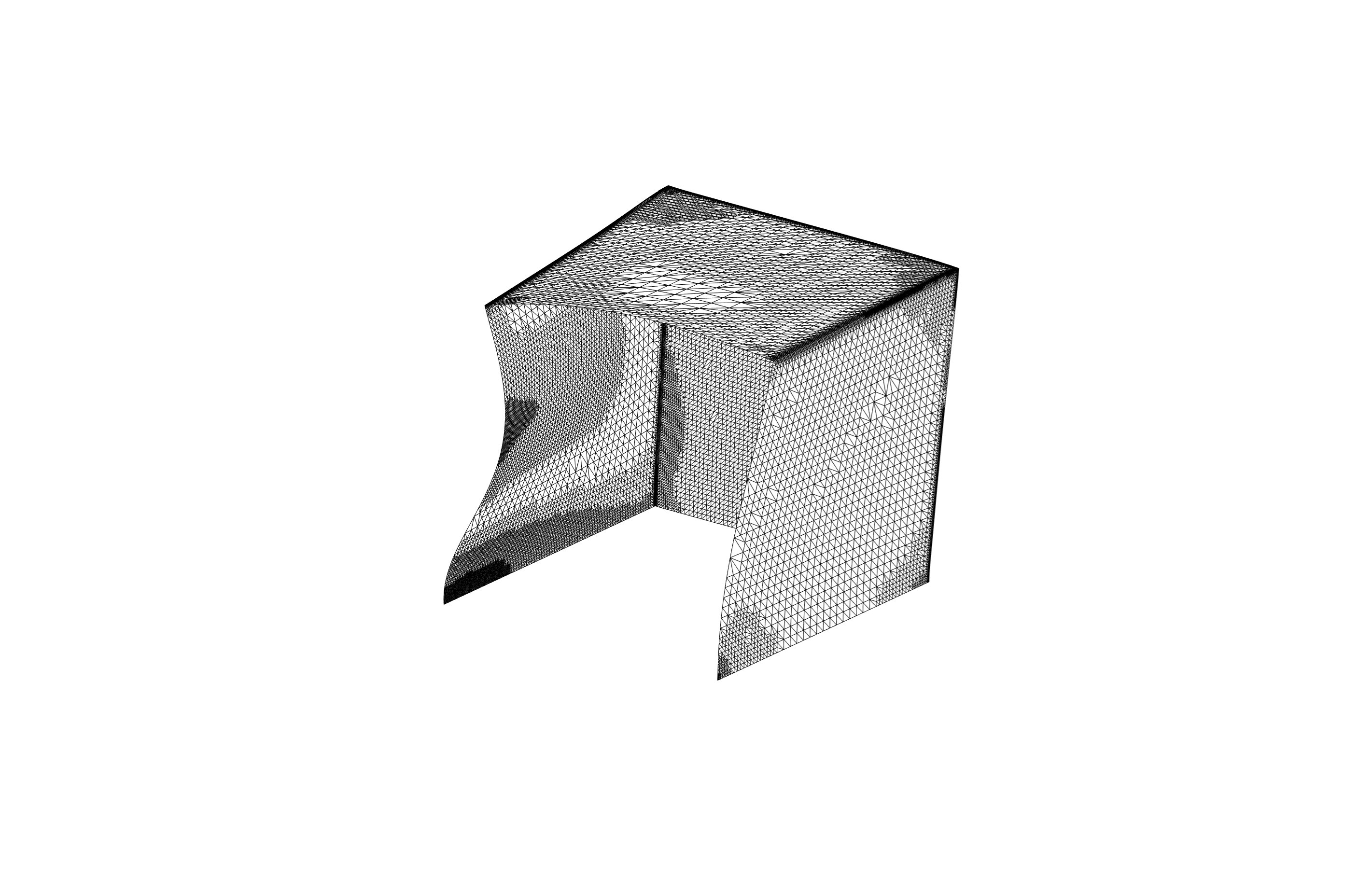 Figure 1
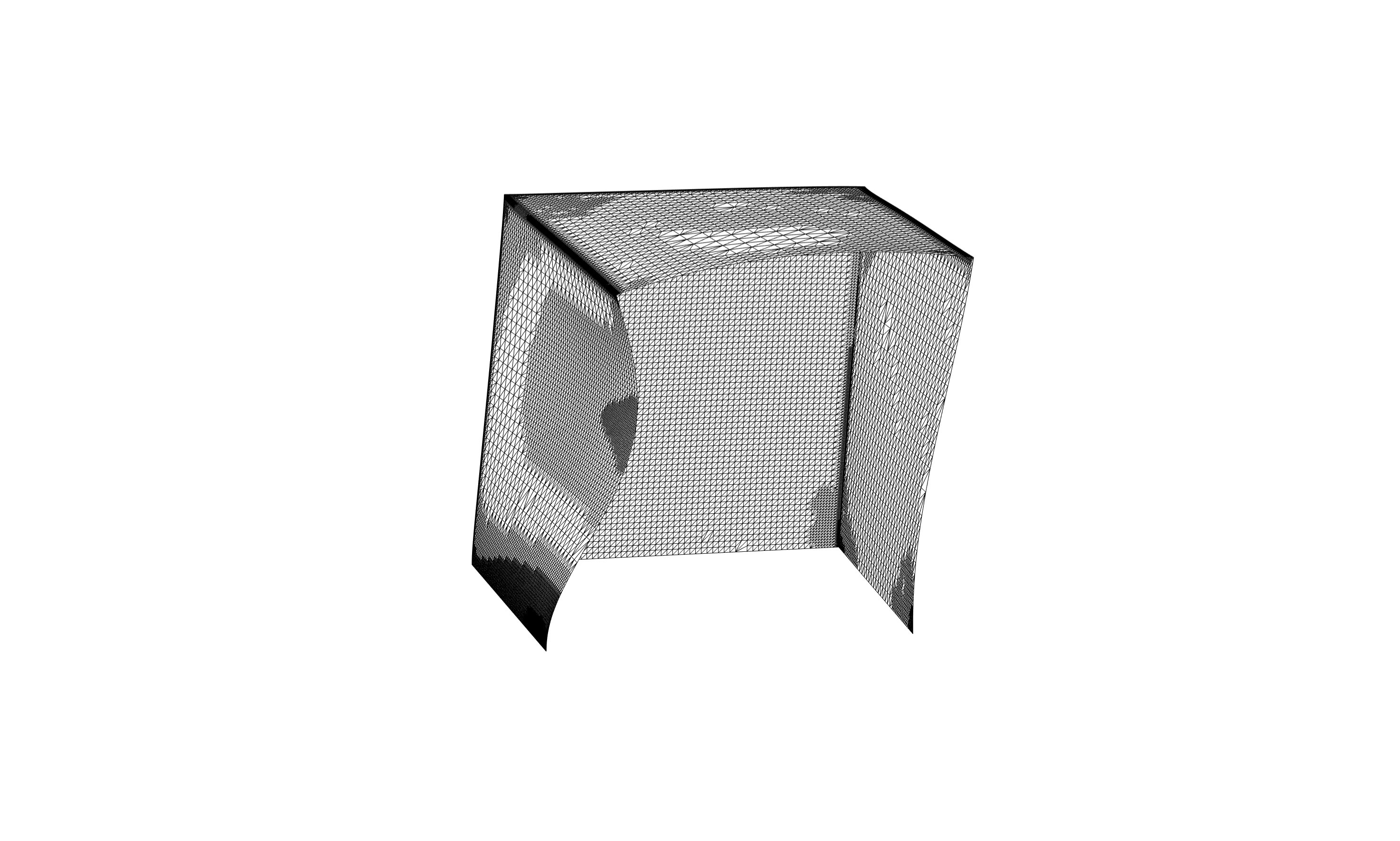 Figure 2
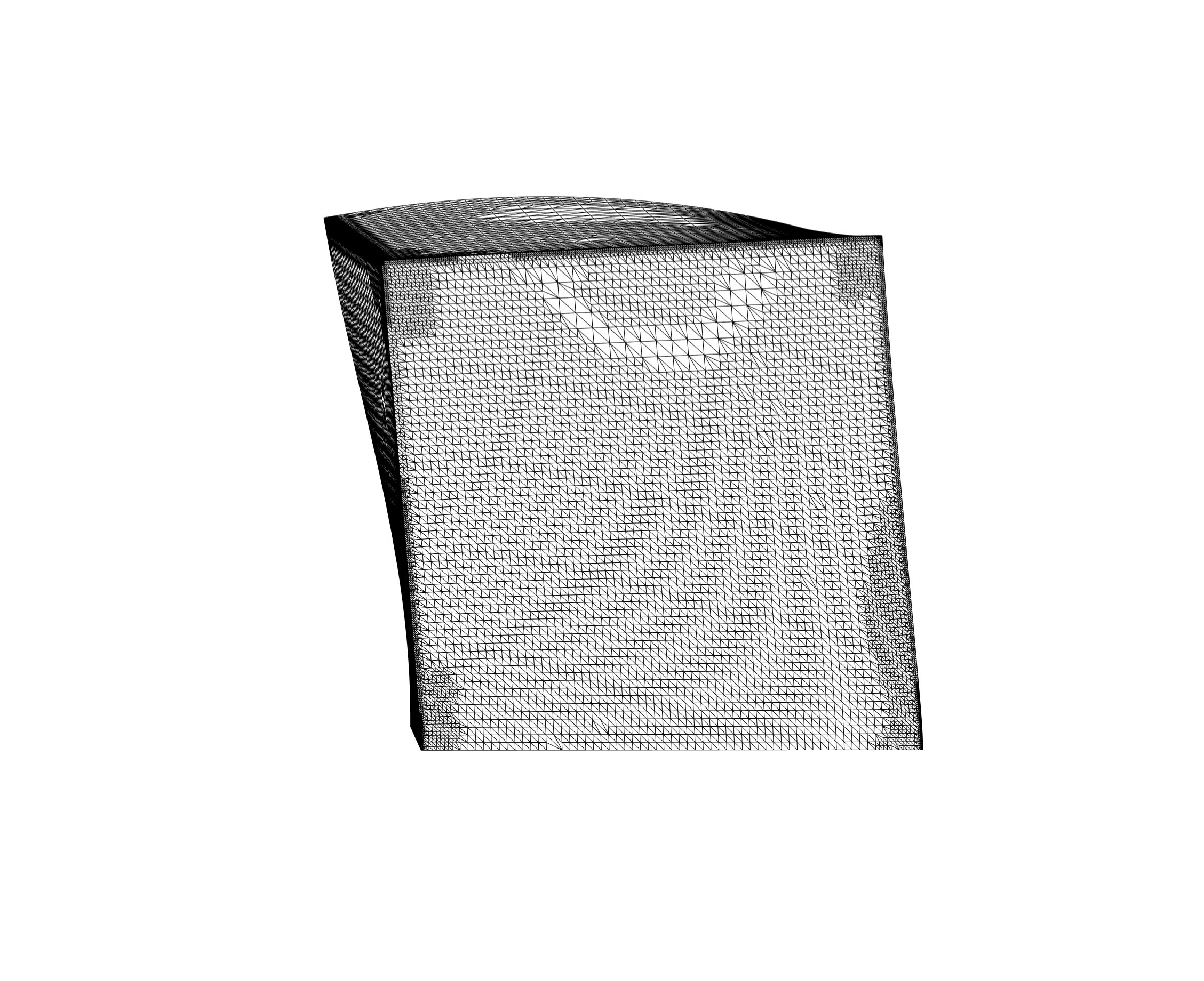 Figure 3
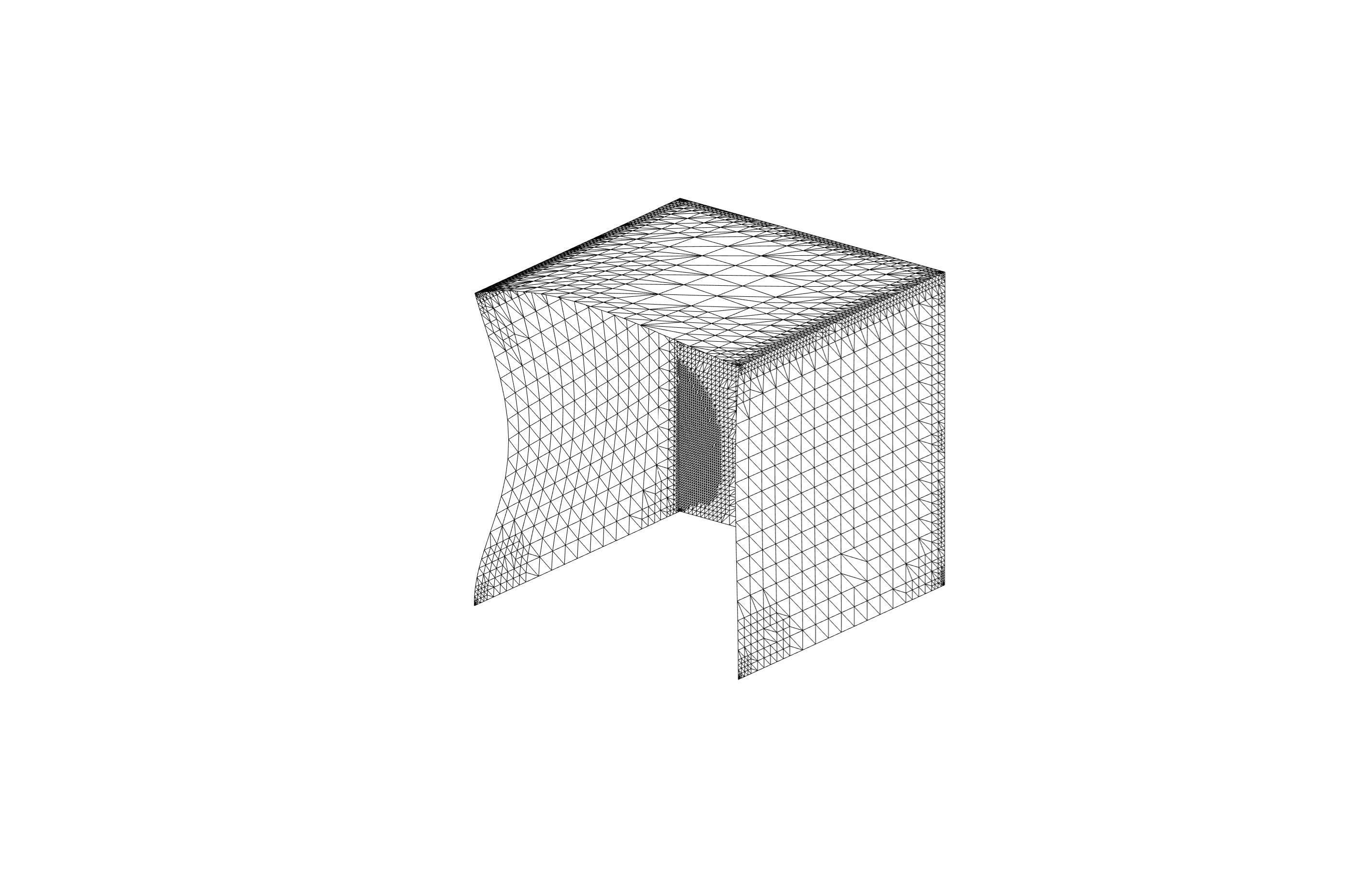 Figure 4
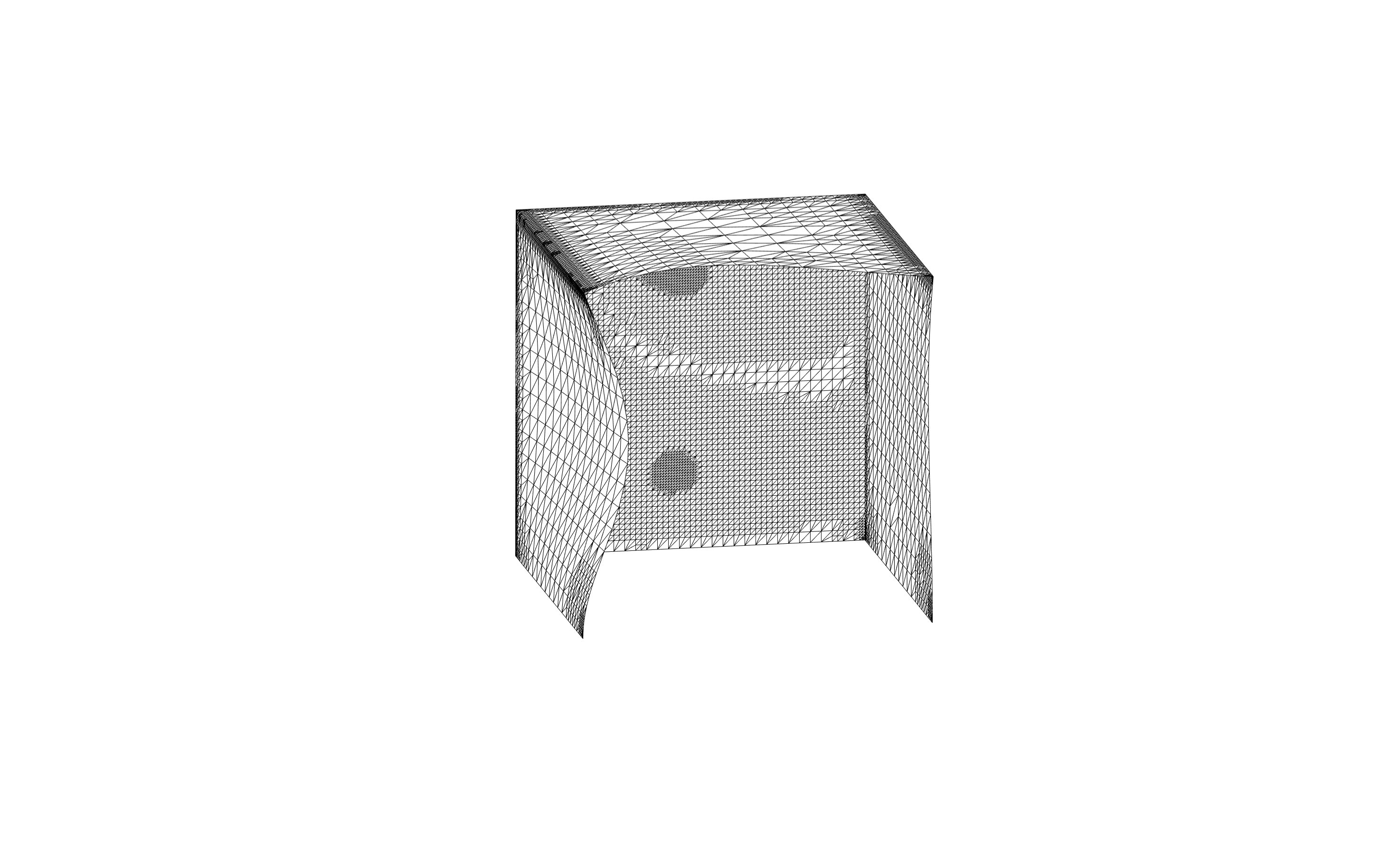 Figure 5
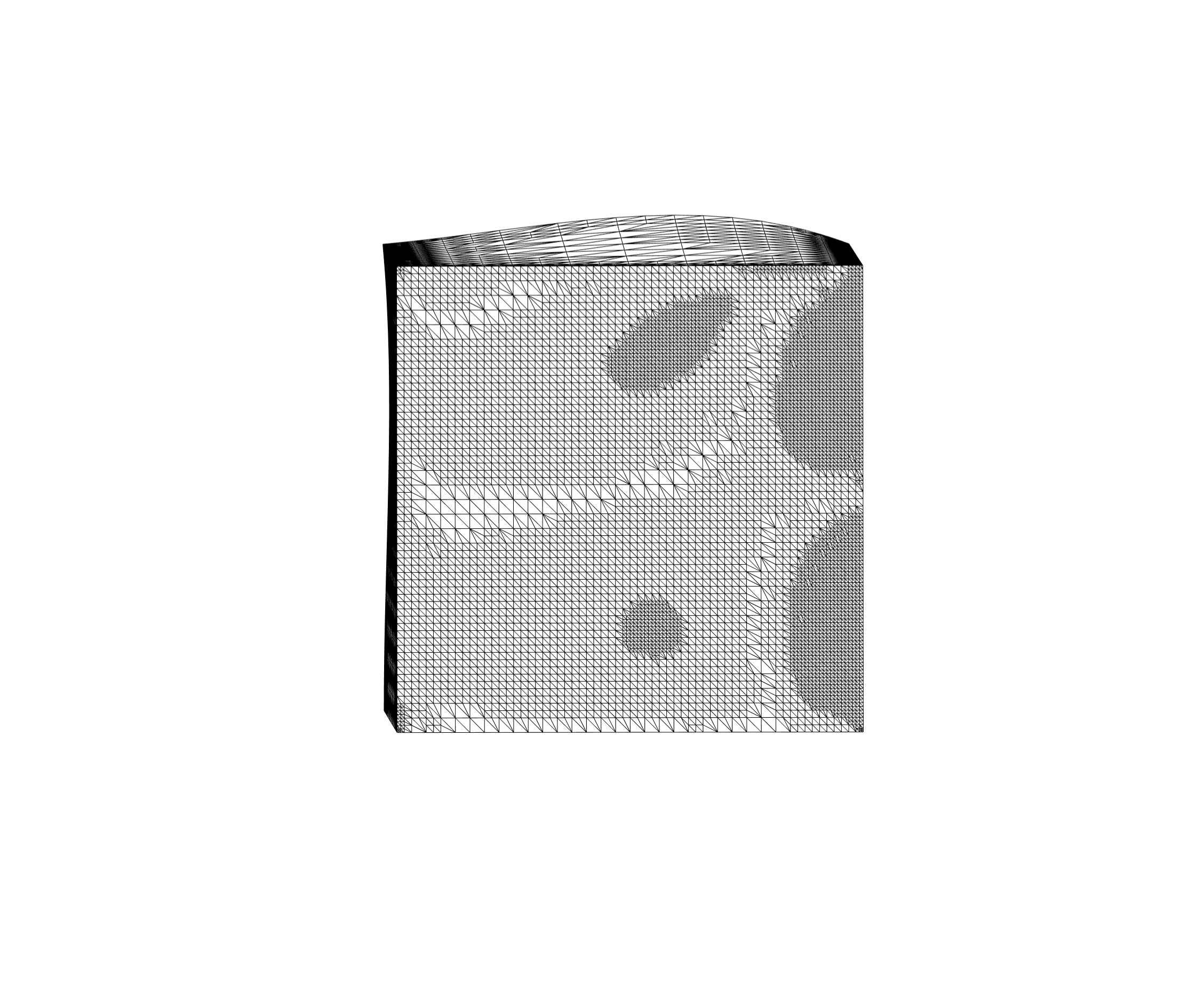 Figure 6
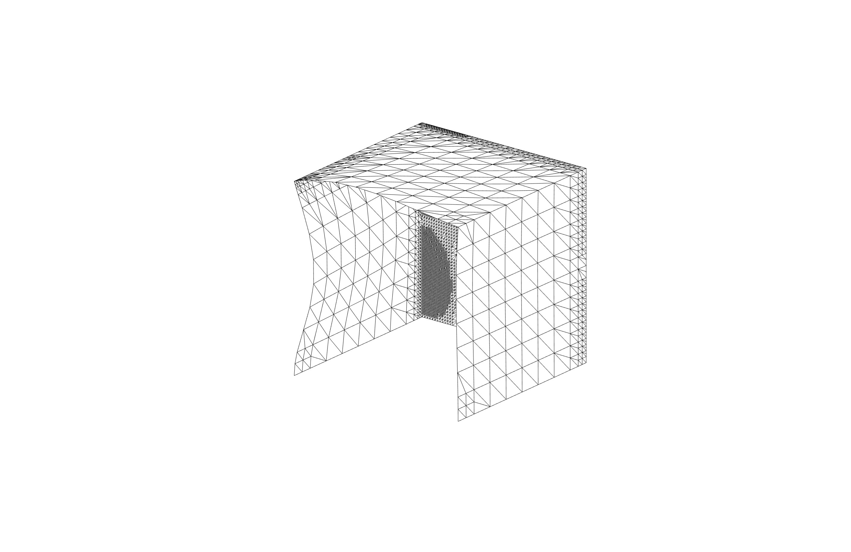 Figure 7
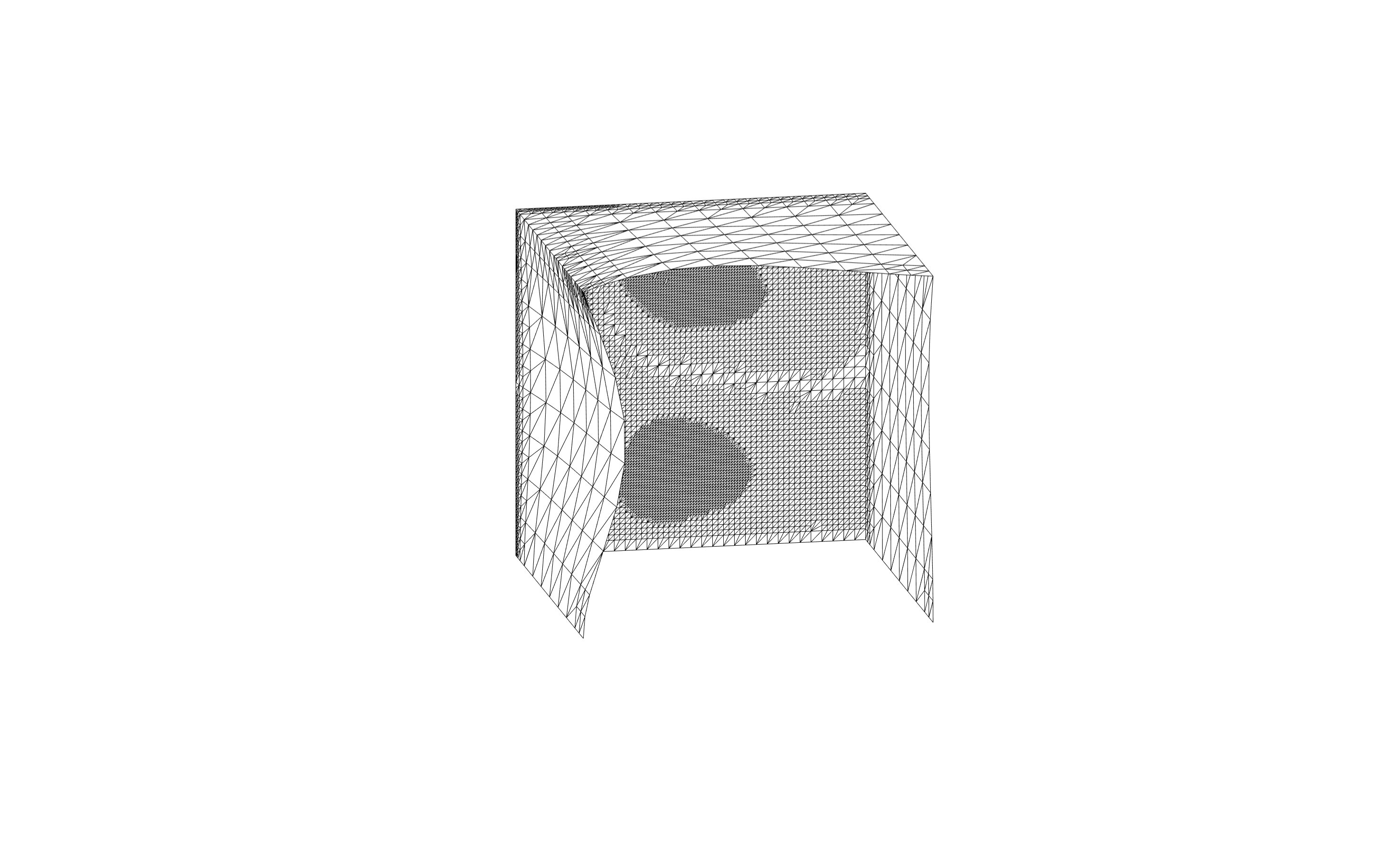 Figure 8
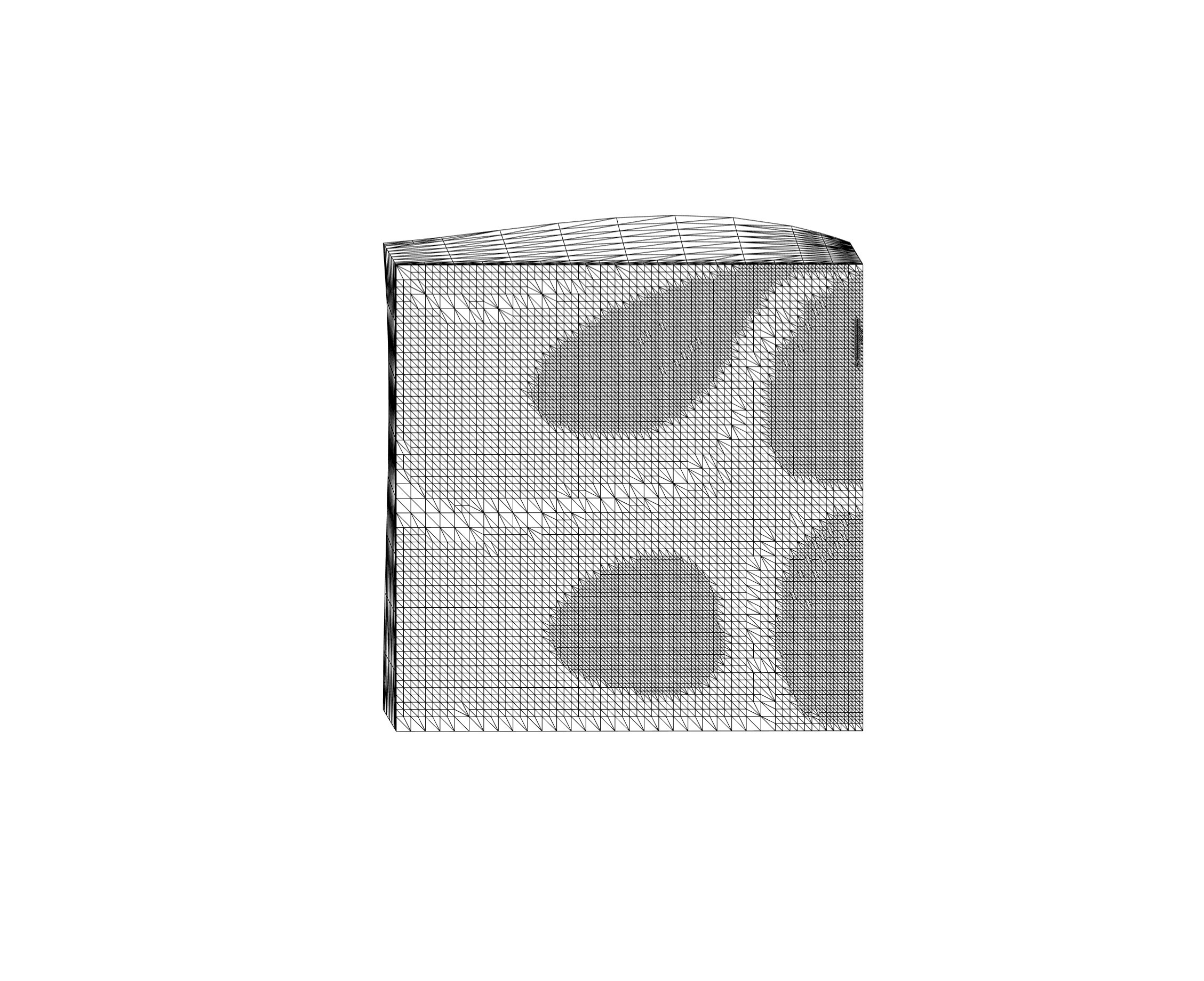 Figure 9
Peer Reviews
No public reviews on file for this paper yet. If you reviewed it on a platform where reviews are public (OpenReview, ICLR, NeurIPS, ICML), you can paste yours below so the community can read it here.
Videos
No videos yet. Explain this paper in a talk, walkthrough, or lecture? Add one.
Taxonomy
TopicsAdvanced Numerical Methods in Computational Mathematics · Elasticity and Material Modeling · Advanced Mathematical Modeling in Engineering
11institutetext: P. Hansbo
Department of Mechanical Engineering, Jönköping University, SE-55111 Jönköping, Sweden
M. G. Larson
Department of Mathematics and Mathematical Statistics, Umeå University, SE–901 87 Umeå, Sweden
Continuous/Discontinuous Finite Element Modelling of Kirchhoff Plate
Structures in Using Tangential Differential Calculus.
Peter Hansbo
Mats G. Larson
Abstract
We employ surface differential calculus to derive models for Kirchhoff plates including in–plane membrane deformations. We also extend our formulation to structures of plates. For solving the resulting set of partial differential equations, we employ a finite element method based on elements that are continuous for the displacements and discontinuous for the rotations, using –elements for the discretisation of the plate as well as for the membrane deformations. Key to the formulation of the method is a convenient definition of jumps and averages of forms that are -linear in terms of the element edge normals.
Keywords:
tangential differential calculus, Kirchhoff plate, plate structure
1 Introduction
The Kirchhoff plate model is a fourth order partial differential equation which requires –continuous elements for constructing conforming finite element methods. To avoid this requirement, nonconforming finite elements can be used; one classical example being the Morley triangle Mo68 which has displacement degrees of freedom in the corner nodes and rotation degrees of freedom at the midpoint of the edges. If we want to solve also for the membrane displacements, it is more straightforward to be able to use only displacement degrees of freedom for both the normal (plate) and tangential (membrane) displacements. To reach this goal, one can instead use the discontinuous Galerkin (dG) method HaLa02 , more efficiently implemented as a –continuous Galerkin method allowing for discontinuous approximation of derivatives, referred to as the continuous/discontinuous Galerkin, or c/dG, method, first suggested by Engel et al. engel02 , and further developed for plate models by Hansbo et al. HaHeLa10 ; HaHeLa11 ; HaLa03 ; HaLa11 and by Wells and Dung WeDu07 . See also Larsson and Larson LaLa17 for error estimates in the case of the biharmonic problem on a surface. To obtain a continuous model, we combine the plate equation for the normal displacements with the tangential differential equation for the membrane from Hansbo and Larson HaLa14a to obtain a structure with both bending resistance and membrane action. This model is then discretised using continuous finite elements for the membrane and c/dG for the plate, using the same order polynomial in both cases.
The standard engineering approach to constructing plate elements arbitrarily oriented in is to use rotation matrices to transform the displacements from a planar element to the actual, common, coordinates, thus transforming the stiffness matrices. In this paper we instead extend the c/dG method to the case of arbitrarily oriented plates, allowing for membrane deformations, directly using Cartesian coordinates in . We argue that this makes it simpler to implement discrete schemes in general, and in particular the discontinuous Galerkin terms on the element borders. It also gives an analytical model directly expressed in equilibrium equations in physical coordinates.
A particular feature of our method is the handling of the trace terms in the c/dG method. In the recent paper on dG for elliptic problems on smooth surfaces by Dedner, Madhavan, and Stinner DeMaSt13 the definition of the normal to the element faces (tangential to the surface), the conormal, was discussed and different variants tested numerically. In our case, where the surface is piecewise smooth (planar), the definition of the conormal at plate junctures is crucial to the equilibrium. It turns out the proper way to define the jumps and averages of trace quantities that are -linear in the conormal is to compute the trace on the left and right side with the respective unit conormals and adjust the sign on one of the sides with . This leads to a generalization of the standard jump and averages in the flat case where a fixed conormal is used for both the left and right side in the definition of the jump. Furthermore, the standard formula, where the jump in a product of two functions is represented as the sum of the two products of the averages and jumps of the two functions, also generalizes to this situation. With these tools at hand we may directly use standard discontinuous Galerkin techniques to derive a finite element method for a plate structure. The resulting method takes the same form as a standard c/dG method for a plate. The only difference is the proper definition of jumps and averages. See also JoLaLa17 , where a similar approach was used for the Laplace-Beltrami operator on a surface with sharp edges.
The outline of the paper is as follows: In Section 2 we derive a variational formulation for a plate with arbitrary orientation in , in Section 3 we define the relevant traces, including forces and moments, define the averages and jumps of -linear forms, and formulate the interface conditions for a plate structure, in Section 4 we formulate the finite element method, in Section 5 we present numerical examples, and finally we conclude with some remarks in Section 6.
2 Single Plate
2.1 Tangential Differential Calculus
Let be a piecewise planar two-dimensional surface imbedded in , with piecewise constant unit normal and boundary , split into a Neumann part where forces and moments are known, and a Dirichlet part where rotations and displacements are known. For ease of presentation we shall assume that and that we have zero displacements and rotations on the boundary. The case of is straightforward to implement and will be used in the numerical examples. Mixed boundary conditions are handled equally straightforward.
If we denote the (piecewise) signed distance function relative to by , for , fulfilling , we can define the domain occupied by the shell by
[TABLE]
where is the thickness of the shell, which for simplicity will be assumed constant. The closest point projection is given by
[TABLE]
the Jacobian matrix of which is
[TABLE]
where is the identity and denotes exterior product. The corresponding linear projector , onto the tangent plane of at , is given by
[TABLE]
and we can then define the surface gradient as
[TABLE]
The surface gradient thus has three components, which we shall denote by
[TABLE]
For a vector valued function , we define the tangential Jacobian matrix as
[TABLE]
and the surface divergence .
2.2 Displacement and Strain
Upon loading, each point , in the plate undergoes a displacement
[TABLE]
where and are vector fields defined on , arbitrary and a tangential vector, on , or with arbitrary. Thus, neglecting in-plane extensions for the moment, we can write
[TABLE]
in . Here .
We introduce the strain tensor as
[TABLE]
and define the symmetric part of the tangential Jacobian as
[TABLE]
The in-plane strain tensor is implemented using the following identity
[TABLE]
If we write
[TABLE]
then
[TABLE]
where
[TABLE]
is the curvature tensor, cf. DeZo95 ; DeZo96 . For planar , is constant, and this simplifies to
[TABLE]
The total in-plane strain tensor is thus given by
[TABLE]
In DeZo95 ; DeZo96 it is also shown that the mid-plane rotation in the absence of shear deformation is given by , and for shear deformable inextensible shells we thus have the shear deformation vector
[TABLE]
It is is also easy to verify that
[TABLE]
so that, since ,
[TABLE]
since is constant; thus
[TABLE]
In the tangential setting, the Kirchhoff assumption of zero shear deformations can therefore be written
[TABLE]
Furthermore, we find that
[TABLE]
and for inextensible plates we get
[TABLE]
and in this case we thus only obtain contributions to the strain energy from the displacement field
[TABLE]
2.3 Variational Formulations
We shall assume isotropic stress–strain relations,
[TABLE]
where is the stress tensor, and plane stress conditions, for which the Lamé parameters and are related to Young’s modulus and Poisson’s ratio via
[TABLE]
For the in-plane stress tensor we find, by projecting (2.29) from left and right,
[TABLE]
The potential energy of the plate is postulated as
[TABLE]
where for second order Cartesian tensors and . Integrating in , we obtain
[TABLE]
Under the assumption of clamped boundary conditions, the corresponding variational problem is to find u_{n}\in H_{0}^{2}(\Gamma)=\{\text{v\in H^{2}(\Gamma)v=\bm{\nu}\cdot\nabla_{\Gamma}v=0\partial\Gamma}\} such that
[TABLE]
for all .
Introducing also membrane deformations, the total potential energy of the plate must take into account both the bending energy and the membrane energy , so that , where
[TABLE]
Since we wish to use a 3D Cartesian vector field we redefine and , make use of (2.17), and introduce the function space
[TABLE]
We are then led to the variational problem of finding such that
[TABLE]
for all . Introducing the notation
[TABLE]
we may write (2.37) in the more compact form
[TABLE]
For implementation purposes we note that for constant
[TABLE]
and
[TABLE]
2.4 Strong Form
The corresponding strong form of the problem is to find such that
[TABLE]
and
[TABLE]
3 Plate Structures
3.1 Forces and Moments
Consider first a subdomain polygonal subdomain of the plate with boundary consisting of line segments . Using Greens formula on we obtain
[TABLE]
where we used the identity and moved the normal to the first slot in the bilinear form. Letting be a unit tangent vector to , we may split the last term on the right hand side of (3.2) in normal and tangent contributions as follows
[TABLE]
where the first term is the bending moment. For the second term on the right hand side (3.3), integrating by parts along one of the line segments , with unit tangent and normal and , we obtain
[TABLE]
where consists of the two end points of the line segment . We introduce the following notation
[TABLE]
for the normal and tangent components of the force and the moment at each of the line segments on . Furthermore, we introduce the corner, or Kirchhoff, forces
[TABLE]
at a corner associated with a line segment , which has as one of its endpoints and is the unit tangent vector to directed into . We then have the identity
[TABLE]
where is the set of corners on the polygonal boundary and is an enumeration of the two linesegments that has as one of its endpoints.
3.2 Jumps and Averages
Consider a line segment shared by two plates and . We note that the force is an valued 1-form in and the moment is an valued 2-form in . More generally let be an valued -linear form in . Then we define the jump and average at by
[TABLE]
Note that when both plates and reside in the same plane and we recover, using linearity and the simplified notation , the standard jump
[TABLE]
and similarly for the average. Finally, let be an valued -linear form in , then we note that is an valued -linear form in and we have the identity
[TABLE]
where for the scalar product is just usual multiplication of scalars. We may verify (3.16) by
[TABLE]
3.3 Interface Conditions
Consider now a plate structure consisting of a finite number of plates such that at most two plates intersect in a common line segment. For simplicity we consider clamped boundary conditions on the boundary of the structure and focus our attention on the interface conditions at the intersections between the plates. For each line segment where two plates and intersect we have the interface conditions
[TABLE]
corresponding to continuity of displacements, continuity of the rotation angle, equilibrium of forces, and equilibrium of moments.
Furthermore, at each corner , not residing on the boundary of the structure, we require equilibrium of the Kirchhoff forces
[TABLE]
where is an enumeration of the line segments that meet in the corner and is the Kirchhoff force emanating from plate , the two plates that meet in line segment . In other words, there are two contributions associated with each line segment, one for each of the two plates that share the line segment.
4 Finite Element Formulation
4.1 The Mesh and Finite Element Space
Let be a reference triangle and let be the space of polynomials of order less or equal to defined on . Let be triangulated with quasi uniform triangulation and mesh parameter such that each triangle is planar (a subparametric formulation). We let denote the set of edges in the triangulation.
We here extend the discontinuous Galerkin method of Dedner et al. DeMaSt13 for the Laplace–Beltrami operator to the case of the plate. We recall that is piecewise planar and thus is a piecewise constant exterior unit normal to .
For the parametrization of we wish to define a map from a reference triangle defined in a local coordinate system to any given triangle on . Thus the coordinates of the discrete surface are functions of the reference coordinates inside each element, . For any given parametrization, we can extend it to by defining
[TABLE]
where and is the normal to .
We consider in particular a finite element parametrization of as
[TABLE]
where are the physical location of the (geometry representing) nodes on the initial midsurface and are affine finite element shape functions on the reference element. (This parametrization is of course exact in the case of a piecewise planar .)
For the approximation of the displacement, we use a constant extension,
[TABLE]
where are the nodal displacements, and are piecewise quadratic shape functions. We employ the usual finite element approximation of the physical derivatives of the chosen basis on the surface, at , in matrix representation, as
[TABLE]
where . This gives, at ,
[TABLE]
By (4.1) we explicitly obtain
[TABLE]
so
[TABLE]
We can now introduce finite element spaces constructed from the basis previously discussed by defining
[TABLE]
We also need the set of interior edges defined by
[TABLE]
and the set of boundary edges on the Dirichlet part of the boundary
[TABLE]
To each interior edge we associate the conormals given by the unique unit vector which is tangent to the surface element , perpendicular to and points outwards with respect to . Note that the conormals may lie in different planes at junctions between different plates. The jump and average of multilinear forms for edges are defined by (3.12). For edges it is convenient to use the notation
[TABLE]
4.2 The Method
Our finite element method takes the form: find such that
[TABLE]
Here the bilinear form is defined by
[TABLE]
with and
[TABLE]
where denotes the scalar product, and
[TABLE]
Here where is an constant, cf. HaLa11 , and we also recall that the factor is included in the definition (3.9) of the moment . The right hand side is given by
[TABLE]
This is a c/dG method closely related to the one studied in HaLa11 , with the difference of being formulated in an arbitrary orientation in , including membrane deformations, and extended to structures of plates.
We note that:
- •
The continuity of displacement (3.22) is strongly enforced since consists of continuous functions.
- •
The continuity of the rotation angle (3.23) is weakly enforced by the discontinuous Galerkin method.
- •
The force equilibrium conditions (3.24) and (3.26) are weakly enforced but does not give rise to any additional terms in the formulation since consists of continuous functions.
- •
The moment equilibrium condition (3.25) is weakly enforced by the discontinuous Galerkin method.
More precisely, consider an edge shared by two elements and . Multiplying the exact equation by a test function and using Green’s formula element wise generates the following contribution at the edge ,
[TABLE]
where and . For the first term we have using the continuity of and (3.6),
[TABLE]
For the second term we note that the integrand may be written
[TABLE]
where we used the fact that is -linear in , see (3.9), and is 1-linear in , and thus is 3-linear in , together with the definition (3.12) of the jump to write the sum as a jump. Next using (3.16) we get
[TABLE]
since according to (3.25). Thus the second term takes the form
[TABLE]
where at last we symmetrized using the fact that the added term is zero by (3.23) and we included the dependency for clarity. We finally note that we have the following identities
[TABLE]
and
[TABLE]
Remark 4.1
We note that the method for a plate structure has the same form as for a single plate since we use the proper definitions of jumps and averages encoded by the conormal.
Remark 4.2
We note that with this formulation, we have Galerkin orthogonality
[TABLE]
which enables us to prove an a priori error estimate of optimal order provided the solution is regular enough using the same techniques as in HaLa02 .
Remark 4.3
For shell modelling, the plate approach can still be used by viewing the shell as an assembly of facet elements. Then we have an elementwise planar approximation of and we use elementwise projections , where is the elementwise constant approximation of . The differential operators are then defined on the discrete surface, e.g, , etc., and replacing the exact differential operators and exact surface by their discrete approximations in (4.12) we obtain a simple shell model.
5 Numerical Examples
We consider the surface of the box , fixed to the floor and with one wall missing. The material data are: Poisson’s ratio and Young’s modulus . The stabilization parameter was set to . An ad hoc residual–based adaptive scheme was used to generate locally refined meshes. The load was given as
[TABLE]
at , elsewhere. The point of the scaling with thickness is that after division by the membrane stiffness will scale with so that the limit of corresponds to the inextensible plate solution. With increasing the membrane effect will become more and more visible. The numerical results using three different thicknesses, , , are given in Figs. 1–3. Note the marked membrane deformations at .
6 Concluding Remarks
In this paper we have introduced a c/dG method for arbitrarily oriented plate structures. Our method is expressed directly in the spatial coordinates, unlike traditional schemes that typically are based on coordinate transformations from planar elements. This leads to a remarkably simple and easy to implement discrete scheme. The c/dG approach also allows for avoiding the use of –continuity, otherwise required by the plate model, by allowing for discontinuous rotations between elements, and the same function space can then be used to model both plate and membrane deformations. We also introduced the proper conormals, mean values, and jumps necessary for handling the discontinuities on the element borders.
Acknowledgements.
This research was supported in part by the Swedish Foundation for Strategic Research Grant No. AM13-0029, the Swedish Research Council Grants Nos. 2011-4992, 2013-4708, and Swedish strategic research programme eSSENCE.
The reference list from the paper itself. Each links out to its DOI / PubMed record.
- 1(1) A. Dedner, P. Madhavan, and B. Stinner. Analysis of the discontinuous Galerkin method for elliptic problems on surfaces. IMA J. Numer. Anal. , 33(3):952–973, 2013.
- 2(2) M. C. Delfour and J.-P. Zolésio. A boundary differential equation for thin shells. J. Differential Equations , 119(2):426–449, 1995.
- 3(3) M. C. Delfour and J.-P. Zolésio. Tangential differential equations for dynamical thin/shallow shells. J. Differential Equations , 128(1):125–167, 1996.
- 4(4) G. Engel, K. Garikipati, T. J. R. Hughes, M. G. Larson, L. Mazzei, and R. L. Taylor. Continuous/discontinuous finite element approximations of fourth-order elliptic problems in structural and continuum mechanics with applications to thin beams and plates, and strain gradient elasticity. Comput. Methods Appl. Mech. Engrg. , 191(34):3669–3750, 2002.
- 5(5) P. Hansbo, D. Heintz, and M. G. Larson. An adaptive finite element method for second-order plate theory. Internat. J. Numer. Methods Engrg. , 81(5):584–603, 2010.
- 6(6) P. Hansbo, D. Heintz, and M. G. Larson. A finite element method with discontinuous rotations for the Mindlin-Reissner plate model. Comput. Methods Appl. Mech. Engrg. , 200(5-8):638–648, 2011.
- 7(7) P. Hansbo and M. G. Larson. A discontinuous Galerkin method for the plate equation. Calcolo , 39(1):41–59, 2002.
- 8(8) P. Hansbo and M. G. Larson. A P 2 superscript 𝑃 2 P^{2} -continuous, P 1 superscript 𝑃 1 P^{1} -discontinuous finite element method for the Mindlin-Reissner plate model. In Numerical mathematics and advanced applications , pages 765–774. Springer Italia, Milan, 2003.