A recursive algorithm for selling at the ultimate maximum in regime-switching models
Yue Liu, Nicolas Privault

TL;DR
This paper introduces a recursive algorithm to compute the optimal stopping value in regime-switching models, enabling analysis of complex boundary functions without relying on Volterra integral equations.
Contribution
It presents a novel recursive numerical method for optimal stopping problems in regime-switching models, especially when boundary functions are non-monotone.
Findings
Effective computation of optimal stopping boundaries in complex regimes
Applicable to models with mixed-sign drifts and non-monotone boundaries
Provides a practical alternative to integral equation approaches
Abstract
We propose a recursive algorithm for the numerical computation of the optimal value function over the stopping times with respect to the filtration of a geometric Brownian motion with Markovian regime switching. This method allows us to determine the boundary functions of the optimal stopping set when no associated Volterra integral equation is available. It applies in particular when regime-switching drifts have mixed signs, in which case the boundary functions may not be monotone.
Click any figure to enlarge with its caption.
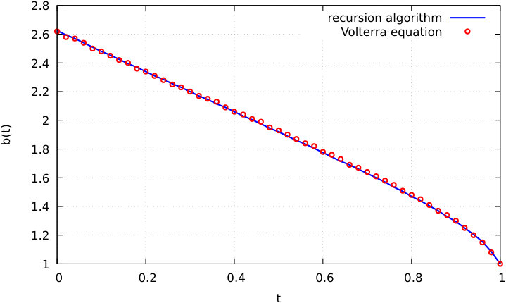 Figure 0
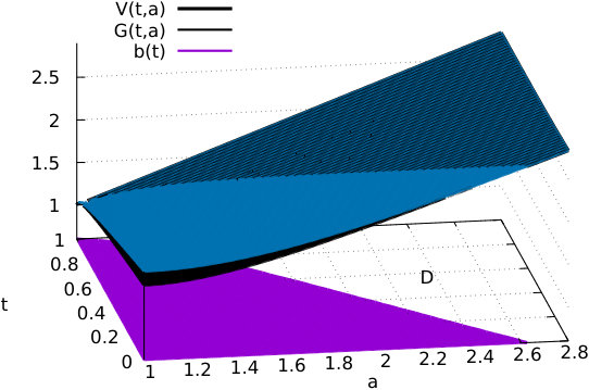 Figure 0
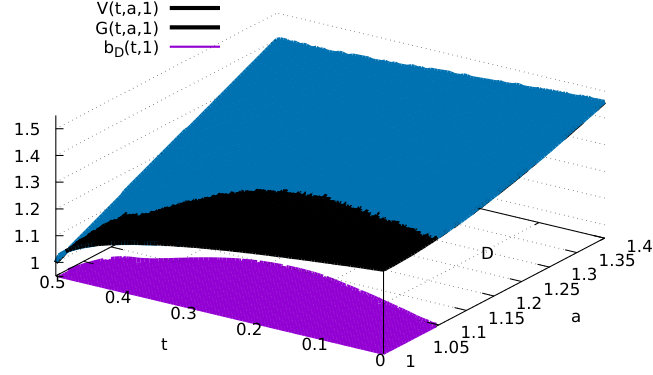 Figure 2
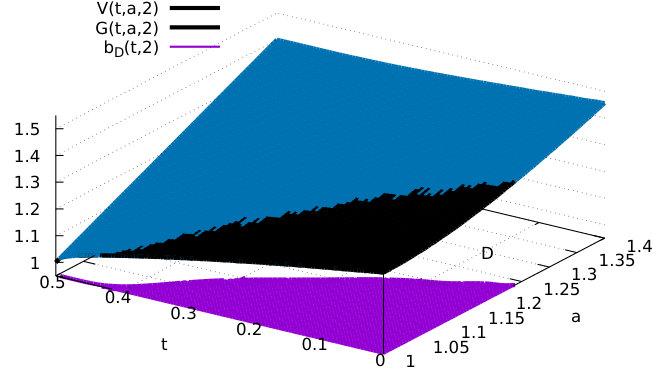 Figure 3
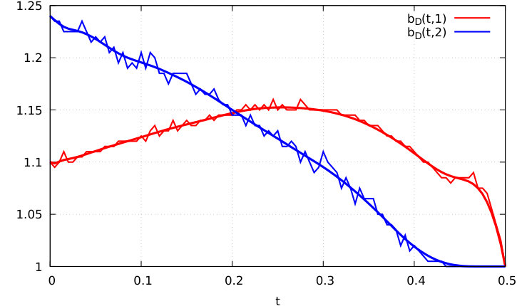 Figure 4
Peer Reviews
No public reviews on file for this paper yet. If you reviewed it on a platform where reviews are public (OpenReview, ICLR, NeurIPS, ICML), you can paste yours below so the community can read it here.
Videos
No videos yet. Explain this paper in a talk, walkthrough, or lecture? Add one.
Taxonomy
TopicsStochastic processes and financial applications · Insurance, Mortality, Demography, Risk Management · Capital Investment and Risk Analysis
A recursive algorithm for selling at the ultimate maximum in regime-switching models
Yue Liu
School of Finance and Economics
Jiangsu University
Zhenjiang 212013
P.R. China
Nicolas Privault
School of Physical and Mathematical Sciences
Nanyang Technological University
21 Nanyang Link
Singapore 637371
Abstract
We propose a recursive algorithm for the numerical computation of the optimal value function \inf_{t\leq\tau\leq T}\mathop{\hbox{\rm I\kern-1.99997ptE}}\nolimits\Big{[}\sup_{0\leq s\leq T}Y_{s}/Y_{\tau}\big{|}{\cal F}_{t}\Big{]} over the stopping times with respect to the filtration of a geometric Brownian motion with Markovian regime switching. This method allows us to determine the boundary functions of the optimal stopping set when no associated Volterra integral equation is available. It applies in particular when regime-switching drifts have mixed signs, in which case the boundary functions may not be monotone.
Key words: *Optimal stopping; Markovian regime switching; non-monotone free boundary; recursive approximation. *
Mathematics Subject Classification (2010): 93E20; 60G40; 60J28; 35R35; 91G80; 91G60.
1 Introduction
The study of optimal stopping of Brownian motion as close as possible to its ultimate maximum has been initiated in Graversen, Peskir and Shiryaev [3]. For geometric Brownian motion, the optimal prediction problem
[TABLE]
of selling at the ultimate maximum over all -stopping times has been solved in [2] by Du Toit and Peskir when the asset price is modeled by a geometric Brownian motion and is filtration generated by , see [10] for background on optimal stopping and free boundary problems, and Chapter VIII therein for ultimate position and maximum problems.
This framework has recently been extended in Liu and Privault [7] to the regime-switching model
[TABLE]
driven by a finite-state, observable continuous-time Markov chain with state space independent of the standard Brownian motion on a filtered probability space , where is the filtration generated by and and , and are deterministic functions.
Regime-switching models were introduced by Hamilton [5] in the framework of time series, in order to model the influence of external market factors. European options have been priced in continuous time regime-switching models by Yao, Zhang and Zhou [12] using a successive approximation algorithm. Optimal stopping for option pricing with regime switching has been dealt with in e.g. Guo [4] and Le and Wang [6].
It has been shown in particular in [2] that the boundary function is nonincreasing and continuous in and satisfies a Volterra integral equation of the form
[TABLE]
, with given terminal condition , where the functions and are specified in [2].
Under regime switching, the optimal boundary functions depend on the regime state of the system, and they may not be monotone if the drift coefficients have switching signs, cf. Figures 3 and 4 in Section 5. Essentially, a boundary function increases when there is sufficient time to switch from a state with negative drift to a state with positive drift and to remain there until maturity, and is decreasing otherwise. We refer to [8] and [9] for other optimal settings that involve non monotone boundary functions.
In the regime switching setting however, no Volterra equation such as (1.3) is available in general for boundary functions, cf. Section 5 and Remark 5.5 of [7]. In addition, the free boundary problem in the regime switching case consists in a system of interacting PDEs, making its direct solution more difficult, cf. Proposition 5.2 in [7]. In Buffington and Elliott [1] a free boundary problem has been solved under an ordering assumption on the boundary functions in the two-state case, see Assumption 3.1 therein, however this condition may not hold in general in our setting, cf. Figure 4 below, and their method is specific to American options.
In this paper we construct a recursive algorithm for the numerical solution of (1.1) in the regime-switching model (1.2), that includes the case where the drifts have nonconstant signs. Our algorithm has a linear complexity in the number of time steps, hence in the absence of regime switching it also performs faster than the resolution of the Volterra equation, which has a quadratic complexity due to the evaluation of the integral in (1.3), cf. Section 5.
We start by recalling the main results of [7]. From Lemma 2.1 in [7], the optimal value function in (1.1) can be written as
[TABLE]
where the function is given by
[TABLE]
for , , , with , , and
[TABLE]
Here, the infimum is taken over all -stopping times , where , . From Proposition 3.1 in [7], given and , , the optimal stopping time for (1.1), or equivalently for (1.5), is the first hitting time
[TABLE]
of the stopping set
[TABLE]
by the process .
The stopping set defined in (1.7) is closed, and its shape can be characterized as
[TABLE]
in terms of the boundary functions defined by
[TABLE]
cf. Proposition 3.2 of [7].
If the condition is not satisfied for all , then may not be decreasing, cf. Figure 4 below. On the other hand, for all leads to , , , which corresponds to immediate exercise, cf. Proposition 5.3 in [7].
In this paper we construct a recursive algorithm for the numerical solution of the optimal stopping problem (1.1), by determining the stopping set from the values of and , cf. Theorem 2.1 and Lemma 4.1 below. As this approach does not rely on the Volterra equation (1.3), it allows us in particular to determine the boundary function without requiring the condition for all as in [7], cf. for example Figure 4 below. In addition we do not rely on closed form expressions as in [2] as they are no longer available in the regime-switching setting.
Our algorithm extends the method of [12] as it applies not only to the computation of expectations, but also to optimal stopping problems. However it differs from [12], even when restricted to expectations of payoff functions , where follows (1.2). In particular, the recursion of [12] is based on the jump times of the Markov chain whereas we apply a discretization of the time interval , and our algorithm requires the Monte Carlo method only for the estimation of (2.3) below.
2 Main results
In the sequel we let , , , , and
[TABLE]
In the following Theorem 2.1, which is proved in Section 3, the function is computed by the backward induction (2.3) starting from the terminal time .
Theorem 2.1
* For all , and , the solution of (1.4) satisfies*
[TABLE]
where is the discrete infimum
[TABLE]
*taken over all -valued stopping times , and . *
* The value of in (2.2) can be computed by the backward induction*
[TABLE]
for , under the terminal condition , , where in defined in (1.6).
In addition, by the following Theorem 2.2 proved in Section 4, we provide a way to approximate the function used in (2.3). In the sequel we denote by
[TABLE]
the joint probability density function of , and we let denote the infinitesimal generator of , and define
[TABLE]
Next, we show in Theorem 2.2 that is approximated by a limiting sequence given by the backward induction (2.6) below.
Theorem 2.2
For any and we have
[TABLE]
where the limit is uniform in and is defined by the backward induction
[TABLE]
, with the terminal condition , , .
In the particular case of constant drift and volatility cf, Theorems 2.1 and 2.2 also provide an alternative numerical solution in the geometric Brownian motion model of [2]. In this case, is computed from (2.3) by the backward induction
[TABLE]
with
[TABLE]
for all and , where , , and is given by (2.4). In the general regime switching setting, the function in (2.7) can be estimated by Monte Carlo, while in the absence of regime switching it can be computed in closed form, cf. (2.7) in [2].
In Sections 3 and 4 we prove Theorems 2.1 and 2.2. Numerical illustrations are presented in Section 5 with and without regime switching. We observe in particular that boundary functions may not be monotone when the drift coefficients , , have different signs.
3 Proof of Theorem 2.1
First, we note that for any -stopping time we have
[TABLE]
, , , since is conditionally independent of
[TABLE]
given , where is the drifted Brownian motion
[TABLE]
and , , is defined in (2.5). Hence by (1.4) we have
[TABLE]
, , , where we used (2.2) and the infimum is taken over all -valued discrete stopping times . Therefore by the continuity of with respect to , cf. e.g. [10], Chap III, §7.1.1 page 130 and §7.4.1 pages 135-136, we obtain
[TABLE]
On the other hand, by (3.1) we have
[TABLE]
, , , where is the infinitesimal generator of . Next, we note that for every stopping time we have , hence converges to uniformly in and pointwise. Hence we have
[TABLE]
, for any stopping time , where we applied Lebesgue’s dominated convergence theorem based on the bounds (3.8) and (b) stated at the end of this section. Hence from (3.4) and (3.5) we find, for any stopping time ,
[TABLE]
where we applied (3.1) and the pathwise continuity of . Hence by (2.2), we obtain
[TABLE]
, which completes the proof of (2.1) by (3.3).
In order to prove (2.3) for , we consider an optimal stopping time such that
[TABLE]
where the infimum is taken over the discrete -valued stopping times , and the existence of is guaranteed by Corollary 2.9 of [10] as in Proposition 3.1 of [7]. We note the induction
[TABLE]
, , where and are defined in (2.2) and (1.6) respectively. By (3.6), this yields
[TABLE]
, where we applied (3.7), the Markov property of and the relation .
We close this section with the proof of the two bounds used for (3.5) above.
- (a)
Letting , we check that, for any stopping time and , we have the bound
[TABLE]
in which the right hand side is integrable for all . 2. (b)
On the other hand we have \mathop{\hbox{\rm I\kern-1.99997ptE}}\nolimits\left[{\hat{Y}_{t,T}}/{\check{Y}_{t,T}}\;\Big{|}\;\beta_{t}=j\right]<\infty since, using the drifted Brownian motion defined in (3.2) we have, using the Cauchy-Schwarz inequality,
[TABLE]
where we conclude to finiteness by conditioning and use of the density (2.4).
4 Proof of Theorem 2.2
We start with two lemmas.
Lemma 4.1
For all , and , we have
[TABLE]
Proof. Let denote the probability measure defined by
[TABLE]
where , , is defined in (2.5), and is the standard Brownian motion under defined in (3.2). From the definition (1.6) of we have
[TABLE]
which allows us to remove the drift component in the supremum . Next, using (4.3) we write
[TABLE]
where
[TABLE]
with for any , and
[TABLE]
By (4.5) we have, for any , , and ,
[TABLE]
where in the first equality we used the fact that the time to the first jump of after is exponentially distributed with parameter given , cf. e.g. § 10.4 in [11]. Next, for , , , and , by (4.6) we see that
[TABLE]
where we used the conditional probability distribution
[TABLE]
computed from the exponential distribution with parameter of the first jump time of the Markov chain started at and the transition matrix of the embedded Markov chain, cf. e.g. § 10.7 of [11]. Hence we conclude to (4.1) by (4.4), (4) and (4.8).
Lemma 4.2
For any , the function is uniformly continuous in , uniformly in , i.e.
[TABLE]
Proof. By (4), for all we have
[TABLE]
hence it suffices to show the continuity in of the above bound. Similarly to (4.3), we have
[TABLE]
, . Next, for any we have
[TABLE]
and similarly by replacing with , thus
[TABLE]
is upper bounded by
[TABLE]
which is -integrable as in (b). Therefore, by dominated convergence we find
[TABLE]
and similarly,
[TABLE]
Combining (4) and (4) we conclude to Lemma 4.2 by a classical uniform continuity argument.
Finally, we proceed to the proof of Theorem 2.2. Let
[TABLE]
with . By (2.6), (4.1) and (4.12) we have
[TABLE]
, where
[TABLE]
with
[TABLE]
Combining (4.13) and (4) yields
[TABLE]
for some constant independent of , hence
[TABLE]
and
[TABLE]
which tends to [math] as tends to infinity by (4.9) in Lemma 4.2. Consequently we have
[TABLE]
for any , , and by Lemma 4.2 it follows that
[TABLE]
uniformly in , for all and .
5 Numerical results
In this section we present numerical estimates obtained from Theorems 2.1 and 2.2 for the boundary functions
[TABLE]
of the stopping set defined in (1.7), in the case of two-state Markov chains with .
Constant drift.
In the absence of regime switching, the recursive algorithm of Theorems 2.1 and 2.2 is applied in Figure 1 to the computation of the value functions and with , , , , and .
Figure 1 allows us in particular to visualize the stopping set defined in (1.7) and the continuation set C=\big{\{}(t,a)\in[0,T]\times[1,\infty)\ :\ V(t,a)<G(t,a)\big{\}}.
In Figure 2 the recursive method is compared to the solution of the Volterra integral equation (1.3) by dichotomy for the computation of the boundary function .
As shown in Figure 2, the recursive and Volterra equation methods yield similar levels of precision. However, increasing the number of time steps will make the Volterra equation method perform slower relative to the recursion method, due to the quadratic complexity of the former and to the linear complexity of the latter.
Drifts with switching signs.
Figure 3 presents the graphs of the value functions obtained from the recursive algorithm of Theorems 2.1 and 2.2 with , , , , , , , and
[TABLE]
Figure 3 also allows us to visualize the stopping set and the continuation set
[TABLE]
The numerical instabilities observed are due to the necessity to check the equality when and are very close to each other. We observe that the corresponding boundary function starting from state is not monotone. Precisely, when time is close to [math] it is better to exercise early because one may switch to state after the average time , in which case the drift takes the negative value . On the other hand, when increases up to the function tends to increase as it makes more sense to wait since we may stay at state with for the remaining average time , which is higher than the remaining time .
The boundary functions are plotted in Figure 4 with spline smoothing. Starting from state we observe the usual decreasing boundary , which here becomes close to [math] before time , since in this case we should exercise immediately as the average time to switch to state exceeds the remaining time until maturity.
Until time we should exercise immediately when switching from state to state at a time such that , while after time the strategy is the opposite if .
The reference list from the paper itself. Each links out to its DOI / PubMed record.
- 1[1] J. Buffington and R.J. Elliott. American options with regime switching. Int. J. Theor. Appl. Finance , 5(5):497–514, 2002.
- 2[2] J. du Toit and G. Peskir. Selling a stock at the ultimate maximum. Ann. Appl. Probab. , 19(3):983–1014, 2009.
- 3[3] S.E. Graversen, G. Peskir, and A.N. Shiryaev. Stopping Brownian motion without anticipation as close as possible to its ultimate maximum. Teor. Veroyatnost. i Primenen. , 45(1):125–136, 2000.
- 4[4] X. Guo. An explicit solution to an optimal stopping problem with regime switching. J. Appl. Probab. , 38(2):464–481, 2001.
- 5[5] J.D. Hamilton. A new approach to the economic analysis of non-stationary time series. Econometrica , 57:357–384, 1989.
- 6[6] H. Le and C. Wang. A finite time horizon optimal stopping problem with regime switching. SIAM J. Control Optim. , 48(8):5193–5213, 2010.
- 7[7] Y. Liu and N. Privault. Selling at the ultimate maximum in a regime switching model. Preprint ar Xiv:1508.06770 v 2, 2016.
- 8[8] G. Peskir and F. Samee. The British put option. Appl. Math. Finance , 18(6):537–563, 2011.