This paper investigates the eigenvalues of the semiclassical Witten Laplacian in cases where the associated Arrhenius numbers are degenerate, extending understanding of spectral properties in such scenarios.
Contribution
It provides new insights into the spectral analysis of the Witten Laplacian when the Arrhenius numbers are not strictly increasing, a case less explored in prior research.
Findings
01
Analysis of eigenvalue behavior in degenerate Arrhenius number cases
02
Extension of spectral theory for Witten Laplacian
03
Identification of conditions affecting eigenvalue degeneracy
Abstract
We study the eigenvalues of the semiclassical Witten Laplacian Δϕ associated to a potential ϕ. We consider the case where the sequence of Arrhenius numbers S1≤…≤Sn associated to ϕ is degenerated, that is the preceding inequality are not necessarily strict.
No public reviews on file for this paper yet. If you reviewed it on a platform where reviews are public (OpenReview, ICLR, NeurIPS, ICML), you can paste yours below so the community can read it here.
Videos
No videos yet. Explain this paper in a talk, walkthrough, or lecture? Add one.
Full text
About small eigenvalues of Witten Laplacian
Laurent Michel
Université de Bordeaux, Institut Mathématique de Bordeaux, France
We study the low lying eigenvalues of the semiclassical Witten Laplacian Δϕ associated with a Morse function ϕ.
We consider the case where the sequence of Arrhenius numbers S1≤…≤Sn associated with ϕ is degenerated, that is the preceding inequalities are not necessarily strict.
Introduced in the early eighties by E. Witten to give an analytical proof of Morse inequalities [21], Witten’s Laplacian appeared recently as the cornerstone of many quantitative studies of metastability for kinetic equations (see e.g. [12, 8, 11, 5]).
One of the simplest examples of metastable dynamics is given by the movement of particle evolving in an energy landscape ϕ and submitted to random forces. The position Xt of such a particle at time t satisfies the over-damped Langevin equation
[TABLE]
where h stands for the temperature of the system and Bt is a Brownian force.111This equation appears for instance in physics to describe the microscopic
evolution of a charged gas assuming the mass of the particles is negligible.
Assuming that the potential ϕ has several wells
a particle starting from a local minimum of the function ϕ can use the random force to jump over a saddle point and reach another energy well.
The famous Eyring-Kramers law describes the
average time to escape from a well in the regime of low temperature h→0.
In his pioneering work [14], Kramers predicted in the simplified one dimensional setting that the average transition
time τϕ from a local minimum m to the nearest saddle point s is exponentially large with respect to h−1, τϕ≃aϕeκϕ/h and he gave additionally formulae for the positive
coefficient κϕ and the prefactor aϕ in terms of the second derivatives of ϕ in points m and s.
Observe that when h→0, this average transition time becomes extremely large, which justifies the terminology of metastable state given to the position m.
In practice, Eyring -Kramers law has very important applications in many domains of science where the trajectory (1.1) is used to implement computational algorithms. In order to compute some thermodynamical quantities
[TABLE]
associated with a measure μ and an observable f, one can introduce any random dynamics Xt ergodic with respect to μ and use
Monte Carlo method to approximate Eμ(f) by the long time average of f along any trajectory (see [17] for introduction to these questions).
In many situations one has dμ(x)=Zhe−ϕ(x)/h for some potential ϕ and the over-damped Langevin dynamics (1.1) fulfills the necessary assumptions.
The time needed by the process Xt to explore the whole space Rd (which insures the validity of the above approximation), is directly linked to the metastable properties discussed previously. Understanding this metastable behavior is then of crucial interest if one needs to evaluate some stopping time or accelerate the convergence for instance.
The first mathematical proof of Eyring-Kramers law in a general setting was obtained recently by a potential theory approach [2] and next by semiclassical methods [8].
This later approach and the link with the Witten Laplacian, can be understood easily by looking at Langevin equation (1.1) at the macroscopic level. Indeed, the evolution
of any statistical distribution ρ(t,x) of particles is governed by the Kramers-Smoluchowski equation
[TABLE]
Writing ρ=e−ϕ/hρ~, the above equation is equivalent to
h∂tρ~+Δϕρ~=0, where
[TABLE]
is the semiclassical Witten Laplacian associated to ϕ.
This operator is known to be non-negative and under confining assumptions on the function ϕ it has a non-trivial kernel corresponding to the global equilibrium of
(1.3).
As a consequence, the behavior of ρ~ when t→∞ is driven by the small eigenvalues of
Δϕ. In particular, any state associated to a small eigenvalue looks stable during very long times.
These are the metastable states and the inverses of the corresponding eigenvalues yield their lifetimes.
In [8], Helffer-Klein-Nier obtained a full description of the small eigenvalues of the Witten Laplacian in a quite general setting.
In terms of Kramers-Smoluchovski equation, their result implies that if the initial probability distribution ρ0 belongs to
L2(e2ϕ/hdx), then the solution ρ of (1.3) converges exponentially fast to the equilibrium probability distribution ch−2e−2ϕ/h (where ch is a normalizing factor)
[TABLE]
Moreover, the rate of convergence λh=hb(h)e−2S/h is described by the Eyring-Kramers law, that is:
S is the biggest height a particle has to pass in order to reach the unique global minimum.
-
the prefactor b(h) has an asymptotic expansion with respect to the parameter h, b(h)∼∑kbkhk and its leading term is given by an explicit formula in terms
of the Hessian of ϕ.
More precisely, the assumptions made in [8] imply that there exist a unique minimum m and a unique saddle point s of ϕ such that S=ϕ(s)−ϕ(m). Then, the leading term of b(h) is
[TABLE]
where μ1(s) denotes the negative eigenvalue of Hess(ϕ)(s). In the case of a double well, this formula is exactly the one predicted by Kramers in his paper [14].
Later on, the method developed in [8] to compute the small eigenvalues of the Witten Laplacian was successfully
used on bounded domains [9], [16] and in the study of semiclassical random walks [1].
However, the range of potential ϕ covered by these papers doesn’t include many cases which are very important in practice.
Roughly speaking, in [8], the author make an assumption on the relative position of minima and saddle points that insures in fine that the small eigenvalues are all of different size. Among the limitations of this assumption, the potential ϕ may not have too much saddle points or minima at the same level.
It turns out that in many physical applications, the energy landscape may not satisfy the above assumption.
In chemical physics, the energy potential of the reaction may have some symmetries in numerous situations.
This is for instance the case when looking at some homogenous systems such as Lennard-Jones clusters (see [20] for example and discussions on this topics).
The aim of this paper is to study the spectral properties of Δϕ in
the case where ϕ is a general Morse function without restriction on the relative position of its minima.
1.2. Heuristics on a simple example
A typical example we have in mind is the following. Suppose that ϕ:Rd→R has n0 minima all at the same level and n1 saddle points all at the same level (see Figure 1.1, where the x represent minima and the o local maxima). Denote by S=ϕ(s)−ϕ(m) the difference of height between any minimum and any saddle point. In order to simplify the situation assume also that the function
Hess(ϕ)(x) has eigenvalues ±1 when x belongs to the set of minima and saddle points.
Such an example doesn’t enter in the framework of [8], however it develops some very interesting behavior.
More precisely, in the very simplified case discussed in this section, a consequence of Theorem 7.1 below is the following
Theorem 1.1**.**
There exists ϵ0>0 and h0>0 such that for all h∈]0,h0], Δϕ has exactly n0 eigenvalues
λk,k=1,…,n0 in the interval [0,ϵ0h].
The lowest eigenvalue is λ1=0 and the other ones have the form
[TABLE]
for all k=2,…,n0. Moreover, the prefactors bk(h) have an classical expansion bk(h)∼∑j=0∞hjbk,j and the leading terms bk,0 are exactly the non zero eigenvalues of the graph G whose vertices are the minima of ϕ and whose edges are the saddle points joining two minima (see Figure 1.1).
In terms of Kramers-Smoluchovski equation, this theorem exhibits some metastable states whose lifetimes (given by the inverse of the above eigenvalues) are quantified by the graph G.
At the level of particle, these new rules of computation can be understood as follows.
Since all the minima are at the same level, the equilibrium state is equidistributed among all the minima. Moreover, since all the saddle points are at the same level, an ergodic trajectory
of (1.1) will visit all the minima in the same time scale, by traveling along the edges of the graph G. The same graph Laplacian was constructed by Landim et al [15] in a discrete setting.
It could look surprising that the coefficients bk do not depend on the second derivative of ϕ as in the usual case of
Eyring-Kramers formula. This is actually due to the normalization assumption made at the beginning of this section. In the case where the Hessian is arbitrary, the above result is still available with a weighted graph instead of G. The weights depend explicitly on the Hessian of ϕ (see Theorem 7.1).
To go further and motivate the object introduced in the next section, let us discuss now what happens if we modify slightly the potential ϕ in the following way. Suppose that ϕ is still like in Figure 1.1 excepted that we modify one of the minimal values (higher or lower). In Figure 1.2, the modified minimum is denoted by A.
Then, we can associate to this potential the two hypergraphs corresponding to minima at the same level and linked by a saddle value (see figure 1.2).
If A is an absolute minimum, then equilibrium distribution is concentrated in A and the prefactor bk(h) will be given by the smallest non zero eigenvalue of the two hypergraphs introduced above (roughly speaking this represents the maximum time needed to reach A).
In the contrary, if A is not a global minimum anymore, the equilibrium state is uniformly distributed among all the minima excepted A.
In order to visit each site of the equilibrium state, an arbitrary particle will necessarily pass through the point A.
This heuristics explains why the computation of the prefactor bk(h) will involve a more complicated procedure describing the interaction between the two hypergraphs via the well A.
The main contribution of this paper is to describe quantitatively this phenomena.
2. Framework and results
Let X be either Rd or a compact manifold of dimension d without boundary and let ϕ:X→R be a smooth Morse function.
Consider the semiclassical Witten Laplacian associated to ϕ:
[TABLE]
where h∈]0,1] denotes the semiclassical parameter.
If X is a compact manifold, the operator Δϕ is selfadjoint with domain H2(X) and its resolvent is compact. In the case X=Rd we make the additional assumption that
there exist C>0 and a compact K⊂Rd such that for all x∈Rd∖K, one has
[TABLE]
Then, Δϕ is essentially selfadjoint on Cc∞(Rd) and thanks to (2.2), there exist h0>0 and c0>0 such that
for all h∈]0,h0], we have
[TABLE]
In both situations X compact or X=Rd, it is well-known that Δϕ is non-negative. Hence
σ(Δϕ)⊂[0,∞[ and it follows from the above remarks that σ(Δϕ)∩[0,c0[ is made of eigenvalues with no accumulation point excepted maybe c0. Moreover
e−ϕ/h is clearly in the kernel of Δϕ and belongs to L2(Rd) thanks to (2.2), so that the lowest eigenvalue of
Δϕ is clearly [math].
Since ϕ is a Morse function (and thanks to assumption (2.2) in the case X=Rd), the set U of critical points is finite. In the following, for p=0,…,d, we will denote by U(p) the set of critical points of ϕ of index p. Hence, U(0) is the set of minima and
U(1) the set of saddle points of ϕ. Throughout the paper, we will denote nj=♯U(j).
From the pioneer work by Witten [21], it is well-known that for small h, there is a correspondance between the small eigenvalues of Δϕ and the critical points of ϕ.
More precisely, by standard localization arguments one can show that there exists ϵ0>0 such that for h>0 small enough, Δϕ has exactly n0 eigenvalues in the interval
[0,ϵ0h] that we denote 0=λ1≤λ2≤…≤λn0. This result is easily proved in
[4] with ϵ0h replaced by h3/2. The proof
with ϵ0h can be found in [10], Prop. 1.7 (see also Prop. 1 of [18] for a self-contained proof). Moreover, these eigenvalues are actually exponentially small, that is
live in an interval [0,e−C/h] for some C>0 (see [7] for a proof).
From a topological point of view, these informations (together with the equivalent estimates for the Witten Laplacian Δϕ(p) acting on p-forms) are sufficient to establish a correspondance between the small eigenvalues of Δϕ(p) and the critical points of ϕ of index p
(this was the key point in the Witten’s proof of Morse inequalities).
However, for applications to the description of metastable dynamics, it is important to get some accurate description of the λj’s. Our main theorem will give some asymptotic of these eigenvalues for any Morse function ϕ, without any assumption on the relative position of minimal and saddle values of ϕ.
Before going further, let us introduce few notations that we use in this paper.
For x0∈X and r>0, introduce the geodesic ball B(x0,r)={x∈X,d(x,x0)<r}.
Throughout, we will say that s is a saddle point if it is a critical point of index 1.
Given a(h),b(h)>0, two functions of the semiclassical parameter, we say that a(h)≍b(h) if there exists some constant
c1,c2>0 such that for all h>0 small one has c1b(h)≤a(h)≤c2b(h).
We say that a family of vectors (a(h))h∈]0,1] in a normed vector space V admits a classical expansion if there exists a sequence
of vectors (an)n∈N independent of h and such that for all N∈N, there exists some constants CN>0 such that
[TABLE]
We denote a(h)∼∑n=0∞hnan.
As we shall see later, we will have to analyze carefully some finite dimensional matrices which are strongly related to the critical points of
ϕ. Given any subsets B1,B2 of U, it will be convenient to introduce the finite dimensional vector space F(Bj)
of real valued functions on Bj. We shall then denote by M(B1,B2) the vector space of linear operators from
F(B1) into F(B2).
2.1. Labelling of minima
Let us now recall the general labelling of minima introduced in [8] and generalized in [11].
The main ingredient is the notion of separating saddle point which is defined as follows.
Given a saddle point s of ϕ, and r>0 small enough, the set
[TABLE]
has exactly two connected components Cj(s,r), j=1,2. The following definition is taken from [11], Definition 4.1.
Definition 2.1**.**
We say that s∈X is a separating saddle point (ssp) if it is a saddle point and if C1(s,r) and C2(s,r)
are contained in two different connected components of
{x∈X,ϕ(x)<ϕ(s)}. We will denote by V(1) the set of ssp.
We say that σ∈R is a separating saddle value (ssv) if it is of the form
σ=ϕ(s) with s∈V(1). We denote Σ=ϕ(V(1)) the set of ssv.
We say that E⊂X is a critical component if there exists
σ∈Σ such that E is a connected component of {ϕ<σ} and if
∂E∩V(1)=∅. We denote by C the set of critical components.
Let us now describe the labelling procedure of [11]. Since ϕ is a Morse function, it has finitely many critical points and so Σ is finite. We denote σ2>σ3>…>σN its elements and for convenience we also introduce a fictive infinite saddle value σ1=+∞ and denote Σ=Σ∪{σ1}.
Starting from σ1, we will recursively associate to each σi a finite family of local minima
(mi,j)j and a finite family of critical components (Ei,j)j (see Figure 2.1).
Let Xσ1={x∈X,ϕ(x)<σ1=∞}=X.
We let m1,1 be any global minimum of ϕ (not necessarily unique) and E1,1=X.
-
Next we consider Xσ2={x∈X,ϕ(x)<σ2}. This is the union of its finitely many connected components. Exactly one of these components contains m1,1 and the other components are denoted by E2,1,…,E2,N2. In each component E2,j, we pick up a point m2,j which is a global minimum of ϕ∣E2,j.
-
Suppose now that the families (mk,j)j and (Ek,j)j have been constructed until rank k=i−1. The set
Xσi={x∈X,ϕ(x)<σi} has again finitely many connected components and we label Ei,j,j=1,…,Ni those of these components that do not contain any mk,l with k<i. In each Ei,j we pick up a point mi,j which is a global minimum of ϕ∣Ei,j. Observe that for all i≥2, the components Ei,j are all critical.
We run the procedure until all the minima have been labelled.
Remark 2.2**.**
The above labelling satisfies the following property. For any σi∈Σ and any connected component Ai of
{ϕ<σi}, there exists a unique (k,l) such that k≤i and mk,l∈Ai.
*Proof. *Let us start with the existence part of the result. If Ai is one of the Ei,j for some j, then take k=i and l=j. Otherwise, this means that in the labelling procedure, Ai already contained a minimum mk,l with k<i.
Let us prove the uniqueness part. Assume that mk,l,mk′,l′∈Ai with k≤k′≤i.
Then Ai∩Ek′,l′=∅ and since Ai is a connected component of {ϕ<σi} with σi≤σk′ it follows that
Ai⊂Ek′,l′. Since mk,l∈Ai, it follows that mk,l∈Ek′,l′ which is impossible unless (k,l)=(k′,l′).
□
Using the above labelling, Hérau-Hitrik-Sjöstrand made some significative progress in [11] (in the more general situation of Kramers-Fokker-Planck operators, but this applies to Witten Laplacian).
First, they showed in Theorem 7.1 that the exponentially small eigenvalues (λm(h))m∈U(0) of Δϕ (indexed by the sequence of local minima) satisfy λm(h)≍he−2S(m)/h for the sequence of Arrhenius numbers (S(m))m∈U(0) defined by
S(mi,j)=σi−f(mi,j) with the above notations. However, their method does not permit to prove that h−1λm(h)e2S(m)/h admits a limit when h→0.
In order to compute the asymptotic expansion of the eigenvalues λm(h), they need to make some additional assumption on the interaction between minima and saddle points (see Assumption 5.1 in [11]). This hypothesis, which is a generalization of the one made in [8], can be formulated as follows with the notations of the preceding section:
Generic Assumption: For all i=1,…,N, j=1,…,Ni, the following hold true:
i)
mi,j is the unique global minimum of the application ϕ∣Ei,j.
ii)
if E is a connected component of {ϕ<σi} such that E∩V(1)=∅, there exists a unique s∈V(1) such that
ϕ(s)=supϕ(E∩V(1)). In particular, ϕ−1(]−∞,ϕ(s)[)∩E is the union of exactly two different connected components.
Throughout the paper, we denote by (GA) this assumption.
Under this assumption, there exists a bijection between U(0) and V(1)∪{s1} where
s1 is a fictive saddle point associated to σ1=∞ and for which by convention ϕ(s1)=∞.
Using this one to one correspondence, the authors exhibit some labelling
U(0)={m1,…,mn0} and V(1)∪{s1}={s1,…,sn0} such that the small eigenvalues
λi(h) are of the form
hbi(h)e−2Si/h with Si=ϕ(si)−ϕ(mi).
Moreover, they prove that the bi(h) have a classical expansion and compute the leading term of this expansion (see Theorem 5.10 in [11]).
As it is stated above, (GA) is not exactly Assumption 5.1 stated in [11]. Indeed, it is supposed in [11] that ii) holds true only for E being a critical component.
However, as indicated by the anonymous referee, we can easily construct some function ϕ satisfying this assumption, for which there is no bijection between U(0) and V(1). To see this, first consider in dimension 1 a potential ϕ with 4 minima mj, j=1,…,4 and 3 saddle points sj, j=1,…,3 such that m1<s1<m2<s2<m3<s3<m4 and such that
ϕ(m1)<ϕ(m4)<ϕ(m2)=ϕ(m3) and ϕ(s1)=ϕ(s2)<ϕ(s3).
Since the component of {ϕ<ϕ(s3)} containing m1 is not critical, this function satisfies Assumption 5.1 in [11]. It doesn’t satisfy (GA) as stated above. In higher dimension, one can easily generalize this construction to obtain potentials satisfying Assumption 5.1 in [11], with a fixed number of minima and an arbitrary large number of separating saddle points (think for instance to many saddle points between the well containing m1 and the well containing m2). This shows that Assumption 5.1 is not sufficient to insure a bijection between minima and separating saddle points.
Let us emphasize that the above remark doesn’t affect the rest of the work done in [11], where we can easily use the above corrected version of Assumption 5.1 .
Let us observe that the Generic Assumption allows some degeneracy in the sequence (Sj), that is there
may exists j such that Sj=Sj+1.
However, (GA) remains restrictive for the following reasons:
It permits only potentials ϕ for which U(0) and V(1)∪{s1} have the same cardinal.
-
The eventual degenerate heights are associated to weakly interacting eigenstates in the following sense. Assume for instance that
Sj=Sj+1 for some j=1,…,n0−1 and modify slightly the function ϕ near the minimum mj. Then the coefficients bj is modified whereas the classical expansion of bj+1 remains unchanged.
Figures 2.3, 2.4 below present some examples of potentials where (GA) is not satisfied.
These examples as well as an example in higher dimension are discussed in detail in section 7.3.
In the present paper, we obtain an asymptotic expansion for the λi(h) for general Morse functions ϕ without any additional assumptions
on the relative position of minima and ssp’s.
2.2. Main result
In order to state our main result, we introduce few notations that will be used throughout the paper.
First, using the above labelling, we define
σ:U(0)→Σ by σ(mi,j)=σi
and S:U(0)→]0,+∞] by S(m)=σ(m)−ϕ(m).
We let S=S(U(0)), then with the notations of the preceding section, we have
[TABLE]
In all the paper, we denote by m=m1,1 the (non necessarily unique) absolute minimum of ϕ that was chosen at the first step of the labelling procedure, and we let
[TABLE]
Using again the above labelling, we can associate a critical component to any local minimum. More precisely, we define
[TABLE]
by E(mi,j)=Ei,j.
Observe that by definition, this application is injective.
Using this map, we can associate to each minimum m∈U(0) a boundary set given by Γ(m)=∂E(m). Thanks to the fact that
ϕ is a smooth Morse function, for any m∈U(0), the set Γ(m) is a finite union of compact sub-manifold of X of dimension d−1 with conic singularities at the saddle points.
For our construction of quasimodes, we also need to introduce the set
[TABLE]
Given m∈U(0), one has σ(m)=σi for some i≥2. Moreover, since σi−1>σi, there exists a unique connected component of
{ϕ<σi−1} that contains m (observe that this component is not necessarily critical). We denote that component by E−(m), and by
[TABLE]
the corresponding application, where Ω(X) is the collection of connected open subsets of X.
Thanks to Remark 2.2, we know that
for any m∈U(0), there exists a
unique m′∈E−(m)∩U(0), denoted by m^(m), such that σ(m′)>σ(m). In particular,
[TABLE]
and we denote by E(m) the connected component of {ϕ<σ(m)} containing m^(m). It holds additionally
E(m)⊂E−(m) and we can easily see that E(m) is always a critical component.
Throughout, we denote by
[TABLE]
and
[TABLE]
the corresponding applications.
The fact that the inequality in (2.8) is large or strict plays an important role in our analysis.
Definition 2.3**.**
Let m∈U(0). We say that m is of type I if ϕ(m^(m))<ϕ(m). If ϕ(m^(m))=ϕ(m), we say that m is of type II.
We will denote
[TABLE]
[TABLE]
We have clearly the following disjoint union U(0)=U(0),I∪U(0),II.
Example 2.4**.**
Let us compute the preceding object in the case of the potential ϕ represented in Figure 2.1. The results are presented in Figure 2.2.
∙* Let us start with the object associated to σ2. By definition, E(m2,1)=E(m2,2)=E(m2,3)=E2, where E2 is the connected component
of {ϕ<σ2} that contains m1,1. Then we have m^(m2,1)=m^(m2,2)=m^(m2,3)=m1,1.*
Since ϕ(m1,1)=ϕ(m2,1)<ϕ(m2,3)<ϕ(m2,2), then m2,1 is of type II, whereas m2,2 and m2,3 are of type I.
∙* Consider now the level σ3. One has E−(m3,1)=E−(m3,2)=E2 and
E−(m3,3)=E−(m3,4)=E2,3. Therefore,
E(m3,1)=E(m3,2)=E3 where E3 is the connected component of {ϕ<σ3} that contains m1,1. Similarly, one has E(m3,3)=E(m3,4)=E3′ where E3′ is the connected component of {ϕ<σ3} that contains m2,3. From this computations, it follows that
m^(m3,1)=m^(m3,2)=m1,1 and since ϕ(m1,1)<ϕ(m3,1)=ϕ(m3,2) it follows that
m3,1 and m3,2 are both of type I. On the other hand, m^(m3,3)=m^(m3,4)=m2,3 and since
ϕ(m2,3)=ϕ(m3,3)<ϕ(m3,4) it follows that m3,3 is of type II and m3,4 of type I.*
∙* Finally, E−(m4,1)=E3, E(m4,1)=E4 as represented on Figure 2.2 and
m^(m4,1)=m1,1. Since ϕ(m1,1)=ϕ(m4,1), it follows that m4,1 is of type II.*
The points of type II play an important role in our analysis.
Given σ∈Σ, let Ωσ=Ωσ0∪Ωσ with
[TABLE]
and Ωσ defined by Ωσ=∅ if σ=σ1 and
[TABLE]
if σ∈Σ.
Definition 2.5**.**
We define an equivalence relation R on U(0) by mRm′ if and only if
[TABLE]
Throughout the paper, we denote by Cl(m) the equivalence class of m for the relation R.
Observe that since m is the only minimum such that σ(m)=∞, then
Cl(m)={m}.
Let us denote by (Uα(0))α∈A the equivalence classes of R
with A a finite set. We have evidently
[TABLE]
We need also to consider the set A defined by A=A∖{α} where Uα(0)={m} is the equivalence class of the absolute minimum chosen for ϕ.
Throughout, we will denote qα=♯Uα(0). We will also use the following partition of Uα(0) for any α∈A:
[TABLE]
Proposition 2.6**.**
Let α∈A. The applications σ,E−,E and m^ are constant on Uα(0).
*Proof. *For σ, it is a direct consequence of the definition.
Suppose now that m,m′∈U(0) satisfy mRm′ and m=m′.
Then, m and m′ belong to the same connected component of {ϕ≤σ(m)}. Hence, the uniqueness part in the definition of E− shows that E−(m)=E−(m′).
Since E−(m)=E−(m′), then the identity m^(m)=m^(m′) follows directly from the definition of m^. This implies automatically
E(m)=E(m′).
□
Thanks to the above proposition, given α∈A, we will denote respectively σ(α),E−(α),E(α) and m^(α) instead of
σ(m),E−(m),E(m), m^(m) for some m∈Uα(0).
Definition 2.7**.**
We say that
α* is of type I, if ϕ(m^(α))<ϕ(m) for all m∈Uα(0)*
-
α* is of type II, if there exists m∈Uα(0) such that ϕ(m^(α))=ϕ(m).*
Recall that the height function S:U(0)→R and the set of heights S=S(U(0)) were defined by (2.3) and above.
For any α∈A, we let
[TABLE]
There exists some integers ν1α<ν2α<…<νp(α)α such that
[TABLE]
In the theorem below we sum up in a rather vague way the description of these eigenvalues that we obtained in Sections 5 and 6.
Theorem 2.8**.**
There exist c>0 and some symmetric positive definite matrices Mα, α∈A such that counted with multiplicity, on has
σ(Δϕ)=⋃α∈Aσ(Mα)(1+O(e−c/h))
with
[TABLE]
for some symmetric positive definite matrices Mα,j having a classical expansion with invertible leading term given in Theorem 5.8.
Let us make a few comments on this theorem.
First, observe that since Mα,j has a classical expansion with invertible leading term M0α,j, then its eigenvalues
ζrα,j, r=1,…,rα,j have a classical expansion
[TABLE]
with ζr,0α,j eigenvalue of the matrix M0α,j.
Compared to previous results obtained under the Generic Assumption, the main difference is that the prefactor ζr,kα,j are more difficult to compute since they are obtained as the eigenvalues of the matrices
Mα,j. When (GA) is satisfied, the Mα,j are 1×1 matrices whose spectrum is direct to obtain. In the general case, this is not true anymore and the construction of the matrices Mα,j is more involved.
In particular, it depends dramatically on the number p(α)=♯S(Uα(0)). Observe that this number is also equal to the number of different values taken by ϕ on the equivalence class Uα(0).
If p(α)=1, the coefficients of Mα,j depend only on the couples (m,s) for which
ϕ(s)−ϕ(m)=Sνjα. Excepted the fact that the different eigenvalues ζrα,j,r=1,…,rα,j are linked together, the situation is similar to that encountered in the generic case. Actually, we prove in appendix that if (GA) is satisfied then Cl(m) is reduced to one point for any m, and in particular p(α)=1 for all α.
In the case where p(α)≥2, the matrix is more difficult to compute. It comes from an application of
Schur complement’s method and it depends on some couples (m,s) for which the height ϕ(s)−ϕ(m) is smaller than Sνjα.
In other words, the lifetime of the metastable state m is not entirely described by the height that is needed to jump over in order to reach
the nearest lower energy position. It depends also on some interactions with some higher energy states that are not present in the classical
Eyring-Kramers formula.
To our knowledge, this is is the first time that such a phenomena is exhibited.
Let us now compute p(α) on explicit examples. Let us fix n=2 and consider the potentials ϕ
given respectively by Figures 2.3, 2.4.
In both cases m^(m2,1)=m^(m2,2)=m^(m2,3)=m1,1 that we denote by m^ for short.
Since ϕ(m^)<ϕ(m2,j) for all j, then there is no point of type II, U(0),II=∅ and hence
Ωσ2={E2,1,E2,2,E2,3}.
Therefore, one can compute easily the equivalence classes of R in both cases:
in the case of Figure 2.3, we have 3 equivalence classes: c1={m1,1}, c2={m2,1,m2,2} and c3={m2,3}.
The potential ϕ is constant on each equivalence class, and hence p(c1)=p(c2)=p(c3)=1.
-
in the case of Figure 2.4, we have 2 equivalence classes: c1={m1,1}, c2={m2,1,m2,2,m2,3}.
The potential ϕ takes two different values on c2: p(c2)=2.
We will come back to these examples at the end of the paper and compute explicitly the spectrum of Δϕ in both cases.
Let us finish this discussion by an example where U(0),II=∅. Consider the potential given by Figure 2.5.
In that case m^(m2,1)=m^(m2,2)=m^(m2,2)=m1,1 that we denote by m^ for short.
Since ϕ(m^)=ϕ(m2,1)=ϕ(m2,2)<ϕ(m2,3), then m2,1 and m2,2 are of type II and m2,3 is of type I.
We still have Ωσ20={E2,1,E2,2,E2,3} but contrary to the previous case
Ωσ2={E2} is non empty. It follows that
Ωσ2={E2,1,E2,2,E2,3,E2} and R admits two equivalence classes:
c1={m1,1}, c2={m2,1,m2,2,m2,3}.
The potential ϕ takes two different values on c2 and hence p(c2)=2.
2.3. General strategy of the proof
Let us recall the general strategy followed in [8]. The starting point is to use the supersymmetric structure of the Witten Laplacian.
For 0≤k≤n, let Ωk(X)=C∞(X,ΛkT∗X) be the space of k-differential forms and denote d:Ωk(X)→Ωk+1(X) the exterior derivative and
d∗:Ωk(X)→Ωk−1(X) its adjoint for the natural pairing.
The Witten complex associated to the function ϕ is defined by the semiclassical weighted de Rham differentiation
[TABLE]
and its adjoint
[TABLE]
Then the semiclassical Witten Laplacian is defined on the forms of any degree by
[TABLE]
When restricted to the space of p-forms we denote this operator by Δϕ(p) (observe that in the case p=0, the above formula yields easily (2.1)).
Then, we have the following intertwining relation
[TABLE]
and its analogous for the coderivative
[TABLE]
For any p=0,…,d, it follows from (2.2) that Δϕ(p) (as an unbounded operator on L2) is essentially self-adjoint on the space of compactly supported smooth forms. We still denote by
Δϕ(p) its unique self-adjoint extension.
Then Δϕ(p) is non-negative and thanks to (2.2), there exists c0>0 such that
σess(Δϕ(p))⊂[c0,+∞[ for any
h>0 small enough (in the case where X is a compact manifold, Δϕ(p) has actually compact resolvent).
Moreover, there exists ϵp>0 such that for h>0 small enough, it has exactly
np eigenvalues in the interval [0,ϵph] where np denotes the number of critical points of index p of ϕ. We shall denote by E(p) the spectral subspace
associated to these small eigenvalues of Δϕ(p). Then dimE(p)=np and relations (2.18), (2.19) show that
[TABLE]
This shows in particular that dϕ,h acts from E(0) into E(1) and we shall denote by L this operator.
Similarly Δϕ(0) acts on E(0) and we denote by M this operator. By (2.17), we get
[TABLE]
The general strategy used in [8] (that we will follow in the present work), is to construct appropriate bases
of E(0) and E(1) in which one can compute handily the singular values of L. The main idea to construct such bases is to build accurate quasimodes for Δϕ and to project them on the spaces E(j). The construction of the quasimodes is performed in Section 3. The quasimodes for 1-forms are the ones constructed in [10]. The main properties of these quasimodes will be recalled in Section 3.3. Concerning the quasimodes on [math]-forms, one can not use the ones constructed in [8] since many important properties that are required for our analysis fail to be true in the present situation (for instance, the quasi-orthogonality). In Section 3.2, we use the partition of U(0) into equivalence classes of R to construct a family of quasimodes on [math]-forms adapted to our setting.
Each quasimode will be associated to a minimum m∈U(0).
In Section 4, we compute the matrix L in the above basis. One arrives to a block diagonal matrix
diag(Lα,α∈A) whose singular values are the singular values of each block.
Section 5 is devoted to the computation of singular values of the above blocks. The main difficulty is that given two minima m,m′ in the same equivalence class, one has not necessarily S(m)=S(m′).
For equivalence classes satisfying this property (that is p(α)=1),
each block Lα of the matrix L has a typical size e−S(α)/h and the situation could be handled quite easily.
But more complicated cases may arise where quasimodes yielding different heights S(m) are interacting. In order to treat the full general case, we
use Schur complement method combined with an induction on p(α). Running the induction step requires to exhibit a specific structure of the matrices under consideration (see Sections 5.1 and 5.2). In Section 5.3, we prove a general result for such matrices that we use to conclude in Section 5.4.
In a separate appendix, we collect several result in linear algebra. We also provide a list of notations used in the paper.
Acknowledgement: The author would like to thank D. Le Peutrec for numerous discussions; in particular for pointing out a fondamental argument in the induction step of the proof of the main result. This paper was written while the author was in leave at Stanford University and U.C. Berkeley.
He was supported by the European Research Council,
ERC-2012-ADG, project number 320845: Semi Classical Analysis of Partial Differential
Equations, by the Stanford Mathematic Department and by the France Berkeley Fund, FBF 2016-0071, Semiclassical study of randomness and dynamics.
3. Construction of adapted quasimodes
3.1. Gathering minima by equivalence class
Let us start this section with a proposition
collecting some elementary facts about E,E− and E.
Proposition 3.1**.**
Let m,m′∈U(0) such that m=m′. Then, we have the following
i)
If σ(m)=σ(m′), then:
i.a)
E(m)∩E(m′)=∅**
i.b)
either E−(m)=E−(m′) or E−(m)∩E−(m′)=∅
i.c)
if E−(m)=E−(m′) then E(m)=E(m′) otherwise E(m)∩E(m′)=∅
2. ii)
If σ(m)>σ(m′), then
ii.a)
either E(m)∩E(m′)=∅ or E−(m′)⊂E(m)
ii.b)
either E−(m)∩E−(m′)=∅ or E−(m′)⊂E−(m)
*Proof. *Let m=m′ be two minima. Assume first that σ(m)=σ(m′)=σ.
Since m=m′ and σ−1(∞)={m}, then one has necessarily m,m′∈U(0). In particular,
E−(ν),E(ν), ν=m,m′ are well-defined.
Moreover, E(m) and E(m′) being two connected components of
{ϕ<σ}, one has either E(m)=E(m′) or E(m)∩E(m′)=∅. Since m=m′ and E is injective, then E(m)∩E(m′)=∅, which proves i.a).
Since E−(m) and E−(m′) are two connected component of the same set {ϕ<τ} for some τ>σ(m), then i.b) is obvious.
Suppose now that E−(m)=E−(m′). Since σ(m)=σ(m′) then m^(m)=m^(m′). Moreover, E(m) being the unique connected component of {ϕ<σ(m)} containing m^(m), we get E(m)=E(m′). If E−(m) and E−(m′) are disjoint, then E(m) and E(m′) are also disjoint since E(m)⊂E−(m) and E(m′)⊂E−(m′). This completes the proof of i.c).
Let us now prove ii) and assume that σ(m)>σ(m′). Once again, since σ−1(∞)={m}, then
m′∈U(0). If E(m′)∩E(m)=∅, then E−(m′)∩E(m)=∅.
Moreover, E−(m′) is a connected component of {ϕ<τ} for some τ≤σ(m). Since E(m) is a connected component of
{ϕ<σ(m)}⊃{ϕ<τ}, then E−(m′)⊂E(m) which proves ii.a).
The point ii.b) is proved by similar arguments.
□
Let us now decompose the set of separating saddle points according to the equivalence classes. Given α∈A, introduce the closed set
[TABLE]
and for any α∈A let
[TABLE]
For any α∈A, let
[TABLE]
and define an application Γα from \wideparenUα(0) into the
closed subsets of X by
Since E(m)⊊E(m^), then the application Γα is slightly different from the application Γ defined in below (2.5).
Observe also that for all m∈\wideparenUα(0), Γα(m) is the boundary of the connected component of
{ϕ<ϕ(s)} that contains m.
Lemma 3.3**.**
The collection (Vα(1))α∈A is a partition of V(1).
Moreover, for all α∈A and s∈Vα(1), there exists m1(s)∈Uα(0) and
m2(s)∈\wideparenUα(0) such that
[TABLE]
One can chose m1,m2 in order that
S(m1)≤S(m2) (that is ϕ(m1)≥ϕ(m2)). Up to permutation, the couple (m1(s),m2(s)) is unique.
*Proof. *Let s∈V(1), then ϕ(s)∈Σ and there exists k≥2 such that ϕ(s)=σk. By definition, there exists two different connected components E1,E2 of {ϕ<σk} such that s∈E1∩E2. From the existence part of Remark 2.2 there exist ml,i∈E1 and ml′,i′∈E2 with l′≤l≤k. Moreover, one has necessarily l=k.
Otherwise σ(ml,i)>σk and since E1∩E2=∅, this would imply that ml′,i′∈E(ml,i) which is impossible since l′≤l.
Hence we have l=k. Therefore E1 is equal to E(ml,i) with ml,i∈Uα(0), which proves that s∈Vα(1). Moreover, E2 is either of the form E2=E(ml′,i′) with ml′,i′∈Uα(0) (if l′=k) or E2=E(ml,i) (if l′<k).
Setting m1(s)=ml,i∈Uα(0) and m2(s)=ml′,i′∈\wideparenUα(0), one has
s∈Γα(m1)∩Γα(m2) and since l≥l′ one has also ϕ(m1)≥ϕ(m2).
Let us now prove that the union of the Vα(1) for α∈A is disjoint.
Suppose that s∈Vα(1)∩Vβ(1). Then σ(α)=ϕ(s)=σ(β). Moreover, there exists
m∈Uα(0) and m′∈Uβ(0) such that s∈E(m)∩E(m′). This proves that mRm′
and hence α=β.
The uniqueness of (m1,m2) up to permutation is obvious.
□
Let us now introduce an extra partition that will be useful in the sequel.
Lemma 3.4**.**
For all
α∈A there exists a partition
Vα(1)=Vα(1),b⊔Vα(1),i
such that the following hold true:
i)
for any s∈Vα(1),i, m1(s) and m2(s) belong to Uα(0).
2. ii)
the set Vα(1),b is non-empty and
for all s∈Vα(1),b one has m1(s)∈Uα(0), m2(s)=m^(α) and
[TABLE]
*Proof. *Define
Vα(1),i={s∈Vα(1),m1(s),m2(s)∈Uα(0)}.
Then i) is true by definition. Moreover, defining
Vα(1),b=Vα(1)∖Vα(1),i, one has automatically the partition property and it remains to prove ii).
Since α∈A, the set
E(α)∩(∪m∈Uα(0)E(m))
is non-empty and contained in Vα(1),b. This proves that Vα(1),b is not empty.
Suppose now that s∈Vα(1),b. It follows from
Lemma 3.3 that m1(s)∈Uα(0) and m2(s)∈Uα(0).
But by definition of Vα(1),b, m2(s) can not belong to
Uα(0), which implies by definition that m2(s)=m^(α). This completes the proof of ii).
□
3.2. Quasimodes for [math]-forms
In this section we construct a family of quasimodes of Δϕ(0) associated to the minima of ϕ. Each of these quasimodes will be of the form
x↦h−4dχm(x)e−(ϕ(x)−ϕ(m))/h with some suitable cut-off functions χm associated to a minimum m∈U(0).
Following [8], we can associate to each minimum m∈U(0) a cut-off function χm in the following way.
For m=m, we simply take χm=1. For m∈U(0) we introduce some small parameters
ϵ,ϵ~,δ>0 with ϵ~<ϵ and
we define
[TABLE]
Proposition 3.5**.**
Let χm be any function in Cc∞(Eϵ,2ϵ~,2δ(m)) such that χm=1 on Eϵ,ϵ~,δ(m).
There exists ϵ0>0, δ0>0 and C>0 such that for all 0<δ<δ0, all 0<ϵ<ϵ0 and all 0<ϵ~<ϵ/4, the following hold
true:
a)
if x∈supp(χm) and ϕ(x)<σ(m), then x∈E(m)
2. b)
there exists cϵ>0 such that for all
x∈supp(∇χm), we have
either x∈/∪s∈V(1)∩Γ(m)B(s,ϵ) and
[TABLE]
-
or x∈∪s∈V(1)∩Γ(m)B(s,ϵ) and
[TABLE]
3. c)
for all s∈U(1)∖(V(1)∩Γ(m)), one has
dist(s,supp∇χm)≥δ.
If moreover s∈supp(χm) then s∈E(m) (in particular χm(s)=1).
4. d)
suppose that m∈Uα(0),α∈A and let s∈V(1)∩supp(χm). Then, there exists β∈A such that σ(β)<σ(α),
s∈Vβ(1) and ∪m′∈Uβ(0)E(m′)⊂{x∈X,χm(x)=1}.
*Proof. *Observe that the construction of the cut-off functions χm is slightly different to that of the χk,ϵ in Proposition 4.2 in [8] (in particular because there can exist more than one separating saddle point on ∂E(m)).
Let δ1=min{∣s−s′∣,s,s′∈U(1),s=s′} and δ2=min{dist(s,Γ(m)),s∈E(m)∩U(1)}.
Let 0<δ<41min(δ1,δ2) and
ϵ0>0 such that there exists C>0 such that for all 0<ϵ<ϵ0 and all s∈V(1), one has
[TABLE]
This is possible since ϕ is a smooth function.
Then a) and b) above can be proved in a similar way as in Proposition 4.2 in [8] and c) is a direct consequence of our choice of
δ.
Let us now prove d). By definition, if s∈V(1)∩supp(χm), then s∈E(m) (here we use the condition 0<ϵ~<ϵ/4). Hence, there exists β=α such that
s∈Vβ(1) and one has additionally σ(β)<σ(α). By definition of the sets E(m), this implies that
∪m′∈Uβ(0)E(m′)⊂E(m)∖∪s′∈V(1)∩Γ(m)B(s′,ϵ) for any ϵ∈]0,ϵ0[
with ϵ0>0 small enough independent of δ. This implies the results.
□
We are now in position to define the quasimodes in a recursive way on the values of σ(α).
We start with the quasimode associated to m. We set
[TABLE]
where c(m,h) is a normalizing constant such that ∥fm∥L2=1.
Due to the fact that ϕ may have several global minima, the function fm(0) does not concentrate
only on m but on the reunion of all global minima. Hence the normalizing factor c(m,h) is computed by adding the contributions coming from each of these minima via quadratic approximation.
More precisely, it follows from the Laplace method that
c(m,h)∼∑k=0∞hkγk(m) with the function γ0 given by
Eventually, observe that fm(0) is an exact quasimode: Δϕfm(0)=0.
-
Suppose now that k∈{2,…,K} and that the quasimodes fm(0) have been constructed for m∈⋃α′∈A,σ(α′)≤σk−1Uα(0), and
let us define fm(0) for m∈Uα(0) with σ(α)=σk.
The form of the quasimode associated to m depends on the type of m as introduced in Definition 2.3.
⋆
If m is of type I, then we define the fm(0) as in [8] by
[TABLE]
where χm is the cut-off function associated to m defined in Proposition 3.5 and c(m,h) is again a normalizing constant such that ∥fm(0)∥L2=1. As before, we have to add all the contributions of minima in E(m) at the same height as m. We get
c(m,h)∼∑k=0∞hkγk(m) with γ0(m) given by (3.8).
⋆
Let us now construct quasimodes associated to minima m of type II. We assume here that U(0),II=∅ and we define
[TABLE]
where for short,
we denote m^=m^(α) and qαII=♯Uα(0),II.
Let us introduce an additional cut-off function around m^ that we define as follows.
Recall that E(α) denotes the connected component of {x∈E−(m),ϕ(x)<σ(m)} that contains m^. As before, we introduce some parameters
ϵ,ϵ~,δ>0 with ϵ~<ϵ and we define
[TABLE]
Then, we let χ^m^ be any function in Cc∞(Eϵ,2ϵ~,2δ(α)) such that χ^m^=1 on Eϵ,ϵ~,δ(α).
For m∈Uα(0),II, we let χ^m=χm, with χm defined in Proposition 3.5.
We want to construct the quasimode as linear combination of the χ^me−ϕ/h, m∈Uα(0),II. In order to chose the coefficients, let us introduce
Fα=F(Uα(0),II) the finite vector space of functions from Uα(0),II into R.
This space has dimension qαII+1 and is endowed with the usual euclidean structure
[TABLE]
We denote by N the associated norm.
Eventually, we define
θ0α∈Fα
by
[TABLE]
where c(m,h) is the unique positive constant such that
the function
[TABLE]
satisfies ∥f~m∥L2=1 and
c0α(h) is defined by N(θ0α)=1.
Let us now extend the definition of the set
H(m) in the following way. Given
α∈A and m∈Uα(0),II we define
[TABLE]
Observe that if α is of type II, since E(m^(α)) is larger than E(α), then
H(m^(α)) and Hα((m^(α)) may be different.
From the preceding definition, it follows that for all m∈Uα(0),II, c(m,h) admits a classical expansion
c(m,h)=∑khkγk(m) with
[TABLE]
Therefore, we can compute the constant c0α(h), and we get
[TABLE]
Here the index α is used to indicate that the function is associated to Uα(0),II.
Lemma 3.6**.**
There exist some functions θ1α,…,θqαIIα∈Fα such that the following hold true:
i)
{θjα,j=0,…,qαII}* is an orthonormal basis of Fα*
ii)
the functions θjα admit a classical expansion
[TABLE]
and for all j≥1, the leading terms θjα,0 are orthogonal to the function
θ0α,0(m)=γ0(m)c0α(0).
*Proof. *First observe that θ0α admits a classical expansion
θ0α∼∑j≥0hjθ0α,j with θ0α,0(m)=γ0(m)c0α(0).
Since (θ0α,0)⊥ is a qαII dimensional subspace of Fα, it admits an orthonormal basis
(θ~jα,0) independent of h. Then the function θ~jα defined by
[TABLE]
form a basis of (θ0α)⊥. Moreover, the θ~jα admit a classical expansion and since
⟨θ~jα,0,θ0α⟩=O(h) for any j, they satisfy
[TABLE]
Defining the (θjα) as the Graam-Schmidt orthonormalization of the (θ~jα), we get the announced result.
□
Observe that since Uα(0),II has qαII elements, the functions θ1α,…,θqαIIα can also be indexed by Uα(0),II using any arbitrary bijection.
We end up with a family of functions (θmα)m∈Uα(0),II and for convenience we will also denote
θm^α=θ0α.
Then, we define the qαII quasimodes associated to the m∈Uα(0),II by
[TABLE]
where the normalization factor c(m′,h) is defined above and insures that
[TABLE]
Before going further and as a preparation for the final analysis we would like to write the quasimode given by (3.9) and
(3.14) in the same fashion.
For this purpose, we define Uα(0)
by
[TABLE]
with the convention that Uα(0),II=∅ if Uα(0),II=∅
(observe that Uα(0) is equal to the set \wideparenUα(0) defined in 3.3 if and only if Uα(0),II=∅).
Then, we define θmα(m′) for any m∈Uα(0),m′∈Uα(0) in the following way:
if m∈Uα(0),II and m′∈Uα(0),II, we keep the above definition.
-
otherwise, we set
[TABLE]
Then formula (3.9) and (3.14) can be summarized in
[TABLE]
with Uα(0) and θα as above.
Definition 3.7**.**
For any α∈A, let us denote by Tα∈M(Uα(0),Uα(0)) the matrix given by
[TABLE]
Let us remark that if all points of Uα(0) are of type I, then Tα is just the qα×qα identity matrix, whereas if
Uα(0),II=∅ it is a (qα+1)×qα matrix.
Observe also that the partitions Uα(0)=Uα(0),I⊔Uα(0),II and
Uα(0)=Uα(0),I⊔Uα(0),II induce decompositions of the corresponding vector spaces
[TABLE]
and
[TABLE]
From the above construction, one deduces that in a suitable basis the matrix Tα is block diagonal with Id on the upper-left corner and a certain orthogonal matrix in the
lower-right corner. More precisely, there exists an orthogonal matrix
\wideparenTα∈M(Uα(0),II,Uα(0),II) such that for any
f=fI+fII with fI∈F(Uα(0),I) and fII∈F(Uα(0),II), one has
[TABLE]
Moreover, the matrix \wideparenTα is just the matrix (θmα(m′))m∈Uα(0),II,m′∈Uα(0),II
whose coefficients are given by Lemma 3.6. In particular, Ran\wideparenTα=(Rθ0α)⊥ where
θ0α is defined by (3.11).
For any m∈U(0), let us introduce the set F(m) defined as follows.
If m=m, let F(m)=X. If m∈U(0),I:=U(0)∩U(0),I, let
F(m)=E(m)
and if m∈U(0),II:=U(0)∩U(0),II let
[TABLE]
where α is such that m∈Uα(0). Observe that we always have E(m)⊂F(m).
Proposition 3.8**.**
Let m,m′∈U(0) be such that m=m′. The following hold true
i)
if mRm′ then
i.a)
if m or m′ is of type I, then F(m)∩F(m′)⊂V(1).
i.b)
if m and m′ are both of type II, then F(m)=F(m′).
2. ii)
If m′∈/Cl(m), then
ii.a)
if σ(m)=σ(m′), then F(m)∩F(m′)=∅.
ii.b)
if σ(m)>σ(m′), then either F(m)∩F(m′)=∅ or
F(m′)⊂F˚(m)
*Proof. *Let mRm′ with m=m′. As in the proof of Proposition 3.1, one has necessarily m,m′=m.
Assume first that m is of type I. Then F(m)=E(m). If m′ is also of type I, then
F(m′)=E(m′). Moreover since m=m′, it follows from i.a) of Proposition 3.1 that
E(m)∩E(m′)=∅. Therefore, F(m)∩F(m′) is either empty or is reduced to a union of saddle points which are separating by definition.
If m′ is of type II, the same proof works. This completes the proof of i.a).
Suppose now that m and m′ are both of type II. Since mRm′, it follows that E(m)=E(m′) and hence F(m)=F(m′)
which shows i.b).
Suppose now that m′∈/Cl(m). Consider first the case where σ(m)=σ(m′). Then, one has necessarily
F(m)∩F(m′)=∅ otherwise we would have mRm′.
Suppose now that σ(m)>σ(m′) and that F(m)∩F(m′)=∅.
If m=m, then F(m)=X and the conclusion is obvious. Suppose now that m∈U(0) and consider first the case where
m and m′ are of type I. Then F(m)=E(m) and F(m′)=E(m′) and since σ(m)>σ(m′) it follows that E(m)∩E(m′)=∅. Hence ii.a) of Proposition 3.1 shows that E−(m′)⊂E(m) which yields F(m′)⊂E(m)=F˚(m). If m is of type I and m′ of type II, then
one has E(m)∩E~=∅ with either E~=E(m′′) for some m′′∈Cl(m′) or E~=E(m′).
As before, E(m) contains the connected component of {ϕ<σ(m)} that contains E~ and the same proof works.
Let us now suppose that m is of type II and m′ is of type I. Then E(m′)∩E~=∅ with either E~=E(m′′)
for some m′′∈Cl(m) or E~=E(m). In both cases one sees easily that
E−(m′)⊂E~ which proves the result.
The case where both m and m′ are of type II is left to the reader.
□
Let us now give some informations on the support of the quasimodes. For m∈U(0), let us introduce the set
[TABLE]
If m is of type I, it is clear that Fϵ,ϵ~,δ(m)=Eϵ,ϵ~,δ(m) and if m is of type II, one has
[TABLE]
From the above construction one deduces the following proposition.
Proposition 3.9**.**
There exists ϵ0,δ0>0 such that for all 0<δ<δ0 and all 0<ϵ~<ϵ/4<ϵ0/4, the following hold true:
i)
for any m,m′∈U(0)
[TABLE]
2. ii)
for any α∈A and m∈Uα(0), one has supp(fm(0))⊂Fϵ,2ϵ~,2δ(m) and
[TABLE]
*Proof. *Observe that
[TABLE]
Since F(m) and F(m′) are compact, the first point of the proposition immediately follows.
The second point of the proposition is a direct consequence of c) of Proposition 3.5.
□
Recall that the functions fm(0),m∈U(0) depend on ϵ,ϵ~,δ via the definition of the cut-off function
χm. This family is quasi-orthonormal in the following sense.
Proposition 3.10**.**
There exists ϵ0,δ0,β>0 such that for all 0<δ<δ0, 0<ϵ~<ϵ/4<ϵ0/4
and all m,m′∈U(0), one has
[TABLE]
*Proof. *Throughout the proof, we assume that 0<δ<δ0 and 0<ϵ~<ϵ/4<ϵ0/4 as in Proposition 3.5 and we decrease ϵ0,δ0 if necessary.
Let m,m′ be two minima.
∙ Consider first the case where mRm′. If m=m, one has necessarily m′=m and hence
⟨fm(0),fm′(0)⟩=∥fm(0)∥2=1 by construction.
Consider now the case where m,m′=m and
suppose first that m or m′ is of type I. If m=m′, the definition of c(m,h) shows that ∥fm∥=1. If m=m′, it follows from
ii) of Proposition 3.9 that fm(0) and fm′(0) are supported in Fϵ,2ϵ~,2δ(m) and Fϵ,2ϵ~,2δ(m′) respectively.
Moreover, thanks to i) of Proposition 3.8, one has F(m)∩F(m′)⊂V(1)∩∂F(m). Hence,
one can chose ϵ0 sufficiently small, so that
Fϵ,2ϵ~,2δ(m)∩Fϵ,2ϵ~,2δ(m′)=∅.
Therefore, supp(fm(0))∩supp(fm′(0))=∅ and hence fm(0) and fm′(0) are orthogonal.
Suppose now that m and m′ are both of type II. Then, we can write
[TABLE]
Since for ν2=ν1, χ^ν1 and χ^ν2 have again disjoint support for ϵ0,δ0>0 small enough, we get
[TABLE]
This shows in particular that ∥fm(0)∥L2=1 for all m∈U(0).
∙ Suppose now, that m′∈/Cl(m) (in particular m=m′). If σ(m′)=σ(m) then F(m)∩F(m′)=∅
thanks to ii.a) of Proposition 3.8 and i) of Proposition 3.9 implies that Fϵ,2ϵ~,2δ(m)∩Fϵ,2ϵ~,2δ(m′)=∅. Then, the first part of ii) of Proposition 3.9
proves that fm(0) and fm′(0) are orthogonal.
Consider now the case where σ(m)=σ(m′), let say σ(m)>σ(m′).
From ii.b) of Proposition 3.8, we know that either F(m′) is disjoint from F(m) or F(m′)⊂F˚(m). In the first case, we get immediately
⟨fm(0),fm′(0)⟩=0 by the same argument as before. Suppose we are in the second situation, that is F(m′)⊂F˚(m). By definition, we have ϕ(m)≤ϕ(m′), and by taking ϵ0,δ0>0 small enough we can insure that Fϵ,2ϵ~,2δ(m′)⊂F˚ϵ,2ϵ~,2δ(m).
Suppose first that ϕ(m)<ϕ(m′). A priori we don’t know if m,m′ are of type I or II. However, since
Fϵ,2ϵ~,2δ(m′)⊂F˚ϵ,2ϵ~,2δ(m), then
[TABLE]
and
[TABLE]
where the constant c~(m,h) is uniformly bounded with respect to h. This is clear if m is of type I. If m is of type II and let say m∈Uα(0),
then F(m′)⊂F˚(m) implies that there exists ν∈Uα(0) such that F(m′)⊂E(ν) (or E(ν)). Then the general formula (3.14) shows (3.23).
Moreover, by construction, there exists
a cut-off function ψ∈Cc∞(F˚ϵ,2ϵ~,2δ(m)) independent of h such that infsuppψϕ=ϕ(m′) and
[TABLE]
and it follows that
[TABLE]
Since ϕ(m′)>ϕ(m), this proves the result.
It remains to study the case where ϕ(m)=ϕ(m′). Let α,α′∈A be such that
m∈Uα(0) and m′∈Uα′(0). From the above assumption, one has also σ(m)>σ(m′)
and F(m′)⊂F˚(m).
Since σ(m)>σ(m′) and ϕ(m)=ϕ(m′) then fm′(0) is necessarily of type II. It has the form (3.14) and since Fϵ,2ϵ~,2δ(m′)⊂F˚ϵ,2ϵ~,2δ(m), then
(3.23) still holds true. Hence, we get
[TABLE]
On the other hand, by a standard argument based on Laplace method, we know that there exist r>0 and β>0 such that for all ν∈Uα′(0),II, one has
Since θm′ is orthogonal to θ0α′ by construction, the first term of the right hand side above vanishes and we get
⟨fm(0),fm′(0)⟩=O(e−β/h). This completes the proof.
□
We end up this section by giving some exponential estimate of the action of dϕ,h on the quasimodes.
Lemma 3.11**.**
There exists C>0 such that for all ϵ>0 small enough, we have
[TABLE]
for all m∈U(0).
*Proof. *The result is classical, but since the quasimodes fm(0) are slightly different from the usual ones, we have to check the estimates.
Let m∈U(0) and let us compute dϕ,hfm(0).
If m=m, then dϕ,hfm(0)=0 and there is nothing to do.
All terms of the above sum corresponding to m∈Uα(0) are O(e−(S(m)−Cϵ)/h thanks to b) of Proposition 3.5.
The only new term is the one corresponding to
m^(m). Since χ^m^∈Cc∞(Eϵ,2ϵ~,2δ) and is equal to 1 on Eϵ,ϵ~,δ, we have again
[TABLE]
on supp(∇χ^m^) and the proof is complete.
□
3.3. Quasimodes for 1-forms
This section is devoted to the quasimodes associated to low lying eigenvalues of Δϕ(1).
The construction of these quasimodes was done in [10] and we refer to that paper for all the proofs.
Here, we just describe the main properties of these functions. In this section ωs denotes a small neighbourhood of s∈U(1) that may be chosen as small as needed independently of ϵ0 fixed in previous sections.
Given any saddle point s∈U(1), and any appropriate open neighborhood ωs of s, let
Pϕ,s denote the operator Δϕ(1) restricted to ωs with Dirichlet boundary conditions.
Let us denote a normalized fundamental state of Pϕ,s. The quasimodes fs(1) are then defined by
[TABLE]
where ψs is a well-chosen C0∞ localization function supported in ωs and equal to 1 near s and
ε0=±1 will be fixed later. By taking ωs sufficiently small,
we can insure that the fs(1) have disjoint supports,
and thanks to c) of Proposition 3.5, we can also shrink ωs in order that
[TABLE]
Observe that this choice of ωs depends on δ0 but not on ϵ0.
From this construction, we immediately deduce that
[TABLE]
and hence the family {fs(1),s∈U(1)} is a free family of 1-forms.
From [7] Proposition 5.2.6, one knows that the eigenvalues of Pϕ,s are exponentially small.
Using Agmon estimates, it follows that
there exists β>0 independent of ε such that
[TABLE]
Combined with the spectral theorem, this proves that the n1 eigenvalues of Δϕ(1) in [0,ϵ1h] are actually
O(e−β/h) (see [7] Proposition 5.2.5, for details).
Furthermore, Theorem 2.5 of [10] implies that these quasimodes have a WKB writing
[TABLE]
where bs(1)(x,h) is a 1-form having a semiclassical asymptotic, and ϕ+,s is the phase generating the outgoing manifold of ∣ξ∣2−∣∇xϕ(x)∣2 at (s,0) (see [6] chapter 3 for details on such constructions). In particular, the phase function ϕ+,s satisfies the eikonal equation ∣∇xϕ+,s∣2=∣∇xϕ∣2 and ϕ+,s(x)≍∣x−s∣2 near s (the notation ≍ was defined in the paragraph before section 2.1). For other properties of ϕ+,s we refer to [10].
3.4. Projection onto the eigenspaces
The next step in our analysis is to project the preceding quasimodes onto the generalized eigenspaces associated to exponentially small eigenvalues. Recall that we have built in the preceding section quasimodes fm(0), m∈U(0) with good orthogonality properties. To each of these quasimode we will associate a function in E(0), the eigenspace associated to o(h) eigenvalues. For this, we first define the spectral projector
[TABLE]
where γ=∂B(0,ϵ0h) and ϵ0>0 is such that σ(Δϕ)∩[0,2ϵ0h]⊂[0,e−C/h].
From the fact that Δϕ(0) is selfadjoint, we get that
[TABLE]
We now introduce the projection of the quasimodes constructed above,
em(0)=Π(0)(fm(0)).
We have the following
Lemma 3.12**.**
The system (em(0))m∈U(0) is free and spans E(0). Besides, there exists β>0 independent of ϵ0 such that
for all 0<ϵ~<ϵ/4<ϵ0/4, one has
[TABLE]
for all m,m′∈U(0).
*Proof. *The argument is very classical. We recall it for reader’s convenience.
One has
[TABLE]
Since (z−Δϕ(0))−1=O(h−1) on γ, it follows from Lemma 3.11 that
em(0)−fm(0)=O(−β/h) for some β>0. This proves the first point. Combining this information with
Proposition 3.10 we get immediately the second point.
□
We can do a similar study for Δϕ(1), for which we know that the n1 eigenvalues lying in [0,ϵ1h] are
actually O(e−α′/h).
To the family of quasimodes (fs(1))s∈U(1), we now associate a family of functions in E(1), the eigenspace associated
to eigenvalues of
Δϕ(1) in [0,ϵ1h]. Thanks to the spectral properties of the selfadjoint operator Δϕ(1), its spectral projector onto E(1) is given by
[TABLE]
where γ=∂B(0,ε1h) with ϵ1 defined above. In the sequel, we denote
es(1)=Π(1)(fs(1)).
The family (es(1))s satisfies the following estimates
Lemma 3.13**.**
The system (es(1))s∈U(1) is free and spans E(1). Besides, we have
[TABLE]
with β′>0 independent of ε.
*Proof. *Using the orthonormality of the fj(1) and (3.29), the proof is the same as that of Lemma 3.12.
□
4. Preliminary for singular values analysis
This section is a preparation to the study of the singular values of the operator L:E(0)→E(1) defined below (2.20).
We simplify the forthcoming study by several reductions and changes of basis.
Let us denote by Lπ the n1×n0 matrix given by
[TABLE]
with es(1), em(0) defined in the preceding section.
Since (em(0)) and (es(1)) are almost orthonormal bases (thanks to Lemma 3.12 and 3.13), this matrix is close to the matrix of the operator L in these bases. We first work on the matrix Lπ.
Recall that m denotes the absolute minimum of ϕ associated to the connected component E(m)=X.
Since Δϕ(0)em=0, the non zero singular values of Lπ are exactly the singular values of the reduced matrix Lπ,′ defined by Ls,mπ,′=Ls,mπ for all s∈U(1),m∈U(0)
with U(0)=U(0)∖{m}.
Lemma 4.1**.**
There exists β′′>0 such that for ϵ>0 sufficiently small, one has
[TABLE]
for all s∈U(1),m∈U(0).
*Proof. *The trick to get the good error estimate above is now well-known (see for instance proof of Prop. 5.8 in [11]) but we recall the proof for reader’s convenience. Let s∈U(1),m∈U(0), then thanks to (2.18) we have
[TABLE]
But from Lemma 3.11, 3.13 and Cauchy-Schwarz inequality one gets
[TABLE]
Since β′ is independent of ϵ, one can conclude by taking ϵ small enough and β′′=β′/2.
□
Let us denote Lbkw∈M(U(0),U(1)) the matrix defined by
[TABLE]
Of course, the first column of this matrix is identically zero and it is more interesting to consider the matrix
Lbkw,′∈M(U(0),U(1)) defined by
[TABLE]
As we shall see later, the singular values of Lπ,′ and Lbkw,′ are exponentially close and it is natural to
study the matrix Lbkw,′.
For s∈U(1)∖V(1) and m∈U(0), thanks to ii) of Proposition 3.9
one has dϕ,hfm(0)=0 near s, and hence
[TABLE]
Therefore, the singular values of Lbkw,′ are equal to the singular values of the reduced matrix Lbkw,′′∈M(U(0),V(1))
defined by
[TABLE]
In order to study this matrix, we need to introduce a new enumeration of critical points.
Let us start with few abstract notations.
Assume that (I,≤) and (J,≤) are two totally ordered sets and let
A=(aij)i∈I,j∈J be the associated matrix (with i,j enumerated in increasing order). Assume that we have partitions PI,PJ of I and J respectively
[TABLE]
Assume that each partition admits a total order ⪯ (that is we can compare the subsets Ii). Then we get a total order ⪯ on I (resp. J) by using the associated lexicographical order:
[TABLE]
Hence, there exists a unique α:(I,≤)→(I,⪯) which is strictly increasing (and hence bijective). Similarly, there is a unique
β:(J,≤)→(J,⪯) which is strictly increasing.
We denote by API,PJ the matrix (aα(i),β(j))i∈I,j∈J.
This matrix is obtained from A by intertwining the basis vector, hence it has exactly the same singular values.
Let us go back to the matrix Lbkw,′′. Consider the partitions of U(0) and V(1) given by
[TABLE]
At this stage of our analysis, we do not need any specific choice of order on these partitions. We just endow A with any total order and for all α,β∈A we choose any arbitrary total order on Uα(0) and Vβ(1).
This gives an order on the above partitions and we
denote by L=(Lα,β)α,β∈A the matrix Lbkw,′′ associated to these partitions. Observe here that each
Lα,β is itself a matrix Lα,β=(Ls,mα,β)s∈Vβ(1),m∈Uα(0).
Lemma 4.2**.**
For all α=β, Lα,β=0.
*Proof. *Let α;β∈A such that α=β and let m∈Uα(0) and
s∈Vβ(1).
If σ(α)=σ(β) then α=β implies that s∈/F(m). Shrinking if necessary (by taking ϵ0,δ0>0 small enough) the support of fm(0) and fs(1), it follows that these functions have disjoint supports so that
their scalar product vanishes.
If σ(α)=σ(β), then by construction dϕ,hfm(0) is supported near {ϕ=σ(α)} whereas
es(1) is supported near {ϕ=σ(β)}. Since this two sets are disjoints we get
⟨fs(1),dϕ,hem(0)⟩=0 and the proof is complete.
□
From this lemma we deduce that the matrix L admits a block-diagonal structure
[TABLE]
with Lα:=Lα,α. Recall from Definition 3.7,
that for any α∈A,
the matrix Tα∈M(Uα(0),Uα(0)) is given by
Tα=(θmα(m′))m′∈Uα(0),m∈Uα(0). We have the following factorization result on Lα.
Lemma 4.3**.**
We have
Lα=LαTα
where the matrix Lα=(ℓ^s,m′α)s,m′∈M(Uα(0),Vα(1)) is given by
[TABLE]
with
gm′(0)(x)=h−4dc(m′,h)χ^m′(x)eϕ(m′)−ϕ(x)/h.
*Proof. *Let s∈Vα(1),m∈Uα(0).
From equation (3.17), one has
[TABLE]
Moreover, the function ϕ being constant on Uα(0),II,
we can replace ϕ(m) by ϕ(m′) in the above identity and it follows that
[TABLE]
which is exactly the result to be proved.
□
One of the crucial points of our analysis is to compute the coefficient ℓ^s,mα. Given m∈Uα(0), we define
[TABLE]
with Hα(m) defined in (3.12). One has clearly hϕ(m)=π4dγ0(m) with
γ0 given by (3.13). Moreover, in the case where
H(m)={m}, one has hϕ(m)=∣detHessϕ(m)∣41.
Given s∈V(1), we denote by λ^1(s) the unique negative eigenvalue of Hessϕ(s).
In order to keep uniform notations, we also extend the definition (4.7) to saddle points by
[TABLE]
Eventually, we introduce the diagonal matrix Ωα∈M(Uα(0),Uα(0)) defined by
[TABLE]
with S^(m)=σ(α)−ϕ(m).
For m∈Uα(0), one has of course σ(α)=σ(m) and hence S^(m)=S(m) but this fails to be true for m=m^(α).
We then define the rescaled matrix
Lα=(ℓ~s,mα)∈M(Uα(0),Vα(1)) by
[TABLE]
i.e.
[TABLE]
Going back to the matrix Lα, one has
[TABLE]
and using the fact that Tαf(m)=f(m) for any f supported on Uα(0),I one gets
[TABLE]
with Ωα∈M(Uα(0),Uα(0)) defined by Ωαf(m)=e−S(m)/hf(m).
The following lemma gives
an asymptotic expansion of the matrix Lα. We recall that m1(s),m2(s) were defined in Lemma 3.3
Lemma 4.4**.**
Let α∈A and s∈Vα(1), m∈Uα(0). The following hold true:
i)
if m∈/{m1(s),m2(s)}, then ℓ~s,mα=0.
2. ii)
the coefficients ℓ~s,mα admits a classical expansion
ℓ~s,mα∼h21∑k≥0hkℓ~s,mα,k. Moreover, one can chose ε0=±1 in
(3.26) in order that the
leading terms satisfy
[TABLE]
and
in the case where m2(s)∈Uα(0),
[TABLE]
In particular, if m2(s)∈Uα(0), one has
[TABLE]
for all s∈Vα(1).
*Proof. *Suppose first that m=m1(s),m2(s).
Then, supp(dϕ,hgm(0))=supp(dχ^m) is contained in a small neighborhood
ω of Γ(m). Since m=m1(s),m2(s) it follows from
Lemma 3.3 that s∈/ω and hence ℓ~s,mα=0 which proves i).
Let us now compute the coefficients ℓ~s,m for m∈{m1(s),m2(s)}∩Uα(0) (observe that this set may be reduced to m1(s)). We compute these coefficients in the case where m2(s)∈Uα(0). If it is not the case, the only non-zero coefficient is ℓ~s,m1(s) that is computed in the same way.
Recall from (3.30), that the quasimodes on 1-forms are given by
[TABLE]
Summing up the construction of [8] section 4.2, there exists an open neighborhood Vs of s on which one can find a system of local Morse coordinates
(y,z)∈R×Rd−1 in which s is the origin and such that the following properties hold true:
(1)
in the above coordinate system one has
[TABLE]
and
[TABLE]
where (λ^j(s))j=1,…,d are the eigenvalues of Hess(ϕ) at point s.
2. (2)
the amplitude bs(1)(x,h) admits a classical expansion
[TABLE]
with
[TABLE]
3. (3)
one can chose the orientation of the y axis so that
[TABLE]
Moreover, the cut-off function χm can be constructed so that
(4)
in Vs the functions χ^mj, j=1,2 depend only on the variable y,
and one can shrink ωs in order that
(5)
supp(fs(1)) is contained in Vs.
Observe that the only minor (but important) difference with [8] is the property (2), saying that each χmj,j=1,2 is supported in one of the two different half plane {y≶0}. Let us now compute the first coefficient in the asymptotic expansion of ℓ~s,mp,α.
Using the above properties, Proposition 3.5 and following the computations of [8] section 6
we get
[TABLE]
with
[TABLE]
Using the local form of ϕ and ϕ+, we get
[TABLE]
with g−(z)=∑j=2dλ^j(s)zj2.
Since χ^m depends only on y and g−≥cν2 on ∣z∣∞≥ν, the integration domain B(s,ϵ) can be replaced by
a smaller one Ws={∣y∣<ϵ,∣z∣∞≤νϵ} modulo exponentially small error terms. Using also the identity
S^(m)=ϕ(s)−ϕ(m), we get
[TABLE]
with
[TABLE]
The integral in the right hand side can be easily computed by mean of Stoke formula and Laplace method.
We get
[TABLE]
Combining this with the expression of c(m,h) and e(s,h), we obtain
[TABLE]
We now remark that with our choice of χ^m, one has
[χ^m1]−ϵϵ=−1 and [χ^m2]−ϵϵ=1.
Taking ε0=(−1)d, we get immediately the formula of ii).
□
5. Computation of the approximated singular values
From Lemma A.2, we know that the singular values of a block-diagonal matrix are given by the singular values of each block. Hence, in view of the results of the preceding section, we study the matrices Lα.
The first step in the analysis is to prove that Lα is injective excepted for α=α.
5.1. Injectivity of the matrix Lα
We first compute the kernel of the matrix Lα.
Lemma 5.1**.**
Let α∈A, then
if α is of type I (that is Uα(0),II=∅), then Lα,0 is injective
-
if α is of type II, then Ker(Lα,0)=Rξ0 where
ξ0∈Rq^α≃Fα is defined by
[TABLE]
for all m∈Uα(0).
*Proof. *Suppose first that α is of type II. Let x∈Fα=F(Uα(0)) be such that
Lα,0x=0, then
Moreover, since α is of type II, then m2(s)∈Uα(0) for any s∈Vα(1)
and thanks to (4.13) we get
[TABLE]
Now, we recall that for any s∈Vα(1), m1(s) and m2(s) are exactly the two minima such that
s=Γα(m1)∩Γα(m2). Therefore, we deduce from (5.2) that
[TABLE]
By definition of the equivalence relation R, this implies that xmhϕ(m) is constant on Uα(0),
which means exactly that x∈Rξ0.
Suppose now that α is of type I and let x∈F(Uα(0)) such that Lα,0x=0. As precedently, one shows that there exists a constant c such that for all m∈Uα(0),
hϕ(m)xm=c.
Recall that the non-empty set Vα(1),b was defined in Lemma 3.4. Given sb∈Vα(1),b, since m2(sb)=m^(α)∈/Uα(0), one has
ℓ~sb,mα,0=0 for any m=m1(sb) and
[TABLE]
Combined with (5.1) this shows that xm1(sb)=0
and hence c=0 which proves that Ker(Lα,0)=0.
□
Proposition 5.2**.**
Let α∈A, then the matrix \wideparenLα:=LαTα admits a classical expansion
\wideparenLα∼h21∑jhj\wideparenLα,j and the matrix \wideparenLα,0 is injective.
*Proof. *Thanks to Lemma 3.6 and 4.4 the matrices Lα and Tα admit some classical expansions
Lα∼h21∑hjLα,j and Tα∼∑hjTα,j. Therefore,
\wideparenLα admits a classical expansions \wideparenLα∼h21∑jhj\wideparenLα,j with \wideparenLα,0=Lα,0Tα,0.
Let us now prove that
\wideparenLα,0 is injective.
Suppose first that α is of type I. Then Tα=Tα,0=Id and the result follows immediately from the first part of Lemma
5.1.
Suppose now that α is of type II and let x∈F(U(0)) be such that
Lα,0Tα,0x=0. We decompose
x=xI+xII with x∙ supported in U(0),∙. Thanks to (3.20), one has
[TABLE]
with \wideparenTα,0:F(U(0),II)→F(U(0),II)
such that Ran\wideparenTα,0=(Rθ0α)⊥ where the function θ0α is defined by (3.11).
On the other hand, one has kerLα,0=Rξ0 and one can decompose
ξ0=ξ0I+ξ0II with ξ0II=θα,0. The equation Lα,0Tα,0x=0 implies that
there exists λ∈R such that Tα,0x=λξ0 and hence
\wideparenTα,0xII=λξ0II. On the other hand, by construction, Ran\wideparenTα,0=(ξ0II)⊥.
This implies that λ=0 and proves the result.
□
Corollary 5.3**.**
For all α∈A the matrix Lα is injective.
*Proof. *This follows directly from the above proposition and the fact that
[TABLE]
with Ωα defined below
(4.10) which is invertible.
□
5.2. Graded structure of the matrices Lα
Throughout this section, we assume that α∈A is fixed.
Recall that we defined Sα=S(Uα(0)), p(α)=♯Sα and some integers
ν1α<…<νp(α)α such that
[TABLE]
with the convention Sν1α>…>Sνp(α)α. In order to lighten the notation we will drop the indices α and write from now p=p(α), νj=νjα.
To the set of heights Sα, we can associate a natural partition
[TABLE]
with
Uα,n(0)={m∈Uα(0),ϕ(m)=σ(α)−Sνn}. We order this partition by deciding that
Uα,n+1(0)≺Uα,n(0).
On the other hand, we recall that Lα=\wideparenLαΩα
with \wideparenLα=LαTα.
Let us
compute the matrices \wideparenLα and Ωα in the basis given by the above partition of Uα(0). With a slight abuse of notation we still denote by \wideparenLα, Ωα the resulting matrices.
Since S^(m)=σ(α)−Sνk on Uα,k(0), it follows from (4.8) that in the above partition,
the matrix Ωα writes
[TABLE]
where the rj=♯Uα,j(0) are such that r1+…+rp=♯Uα(0). Factorizing by e−Sνp/h, we get
Ωα=e−Sνp/h\wideparenΩα(τ) with
[TABLE]
where τ=(τ2,…,τp)∈(R+∗)p is defined by τj=e(Sνp−(j−2)−Sνp−(j−1))/h for any j=2,…,p.
With these new notations, one deduces from (5.3), that
Lα,∗Lα=he−2Sνp/h\wideparenMα(τ)
with
[TABLE]
It turns out that matrix such matrices can be described in a slightly more general setting that is useful to compute their spectrum. We introduce this setting now. Throughout, we denote by S+(E) the set of symmetric positive definite matrix on a vector space E. We will denote by Scl+(E) the set of h-depending matrices M(h)∈S+(E) admitting a classical expansion
M(h)∼∑jhjMj with M0∈S+(E). We will sometimes forget E and write for short S+,Scl+.
Definition 5.4**.**
Let E=(Ej)j=1,…,p be a sequence of finite dimensional vector spaces Ej of dimension rj>0, let
E=⊕j=1,…,pEj and let τ=(τ2,…,τp)∈(R+∗)p−1. Suppose that τ↦M(τ) is a smooth map from (R+∗)p−1 into the set of matrices
M(E).
We say that M(τ) is an (E,τ)-graded matrix if there exists
M′∈S+(E) independent of τ such that M(τ)=Ω(τ)M′Ω(τ) with Ω(τ)∈M(E) of the form (5.6), that is Ω=diag(εj(τ)Irj,j=1,…,p) where
ε1(τ)=1 and εj(τ)=(∏k=2jτk) for all j≥2.
-
We say that a family of (E,τ)-graded matrices Mh(τ), h∈]0,h0] is classical if one has
Mh(τ)=Ω(τ)M′(h)Ω(τ) for some matrix M′(h)∈Scl+(E).
Throughout, we denote by G(E,τ) the set of (E,τ)-graded matrices and by Gcl(E,τ) the set of classical (E,τ)-graded matrices.
Let us remark that for p=1, a graded matrix is simply a τ-independent symmetric positive definite matrix.
Lemma 5.5**.**
Suppose that Mh(τ) is a classical (E,τ)-graded family of matrices and that p≥2. Then
one has
[TABLE]
with
J(h)∈Scl+(E1)**
-
Nh(τ′)∈Gcl(E′,τ′)* with τ′=(τ3,…,τp) and E′=(Ej)j=2,…,p.*
-
Bh(τ′)∈M(E1,⊕j=2pEj)* satisfies*
[TABLE]
with bj(h):E1→Ej independent of τ admitting a classical expansion.
Moreover, the matrix Nh(τ′)−Bh(τ′)J(h)−1Bh(τ′)∗ belongs to Gcl(E′,τ′).
*Proof. *Assume that Mh(τ)=Ω(τ)M′(h)Ω(τ) with Ω(τ) of the form (5.6).
First observe that
[TABLE]
with
[TABLE]
On the other hand, we can write
[TABLE]
with
J(h),N′(h)∈Scl+ and B′(h) admitting a classical expansion.
Therefore,
[TABLE]
which has exactly the form (5.8) with Bh(τ′)=Ω′(τ′)B′(h) and
Nh(τ′)=Ω′(τ′)N′(h)Ω′(τ′).
By construction, Nh(τ′) belongs to Gcl(E′,τ′) and Bh(τ′) has the required form.
It remains to prove that Rh:=Nh(τ′)−Bh(τ′)J(h)−1Bh(τ′)∗ belongs to Gcl(E′,τ′). First observe that since J(h) is symmetric positive definite, this quantity is well-defined. Moreover, one has by construction
[TABLE]
with R′(h)=N′(h)−B′(h)J(h)−1B′(h)∗.
Since J(h)∈Scl+, then J(h)−1∈Scl+ and R′(h) admits a classical expansion R′(h)∼∑jhjRj′ with
[TABLE]
Moreover, since M′(h)∈Scl+ then the matrix
[TABLE]
is symmetric definite positive. Hence, it follows directly from Lemma A.5 that R0′∈S+.
□
5.3. The spectrum of graded matrices
Using Lemma 5.5, we define an application R:Gcl(E,τ)→Gcl(E′,τ′) with τ′=(τ3,…,τp) and
E′=⊕j=2pEj, by
[TABLE]
for any Mh(τ)∈Gcl(E,τ). Of course, the map R depends on E and τ, but we ommit this dependance since the set on which R is acting will be obvious in the sequel. By a slight abuse of notations we will denote
Rk=R∘…∘R (k times). Obviously, Rk acts from G(E,τ) into
G(E(k),τ(k)) with E(k)=⊕j=k+1pEj and τ(k)=(τk+2,…,τp).
In the same way, we defined R, we can define a map J:Gcl(E,τ)→Scl+(E1) by J(Mh(τ))=Mh if p=1 and J(Mh(τ))=J(h) for any Mh(τ) having the form (5.8) if p≥2.
Theorem 5.6**.**
Let E=(Ej)j=1,…,p be a finite sequence of vector space Ej of finite dimension nj=dimEj
and let τ=(τ2,…,τp)∈(R+∗)p−1. Suppose that Mh(τ) is classical (E,τ)-graded. There exists h0>0 and δ>0 such that
uniformly with respect to h∈]0,h0] and ∣τ∣∞<δ, one has
In the above theorem, the matrix J∘Rj−1(Mh(τ)) is always independent of the parameter τ. Let us denote
{λ1j≤…≤λnjj}=σ(J∘Rj−1(Mh(τ)).
The identity (5.10) means that there exists a,b>0 independent of τ,h such that
[TABLE]
and that for all j=1,…,p, Mh(τ) has exactly nj eigenvalues μ1j≤…≤μnjj
in εj[a,b] and
[TABLE]
*Proof. *We prove the theorem by induction on p. Throughout the proof the notation O(.) is uniform with respect to the parameters h and τ.
For p=1, Mh(τ)=Mh∈Scl+(E1) is independent of τ and JR0(Mh(τ))=JMh(τ)=Mh
which proves the statement.
Suppose now that p≥2 and
let Mh(τ)∈Gcl(E,τ). We have
[TABLE]
with J(h),Bh(τ′) and Nh(τ′) as in Lemma 5.5.
In order to lighten the notation we will drop the variable τ,τ′ in the proof below.
For λ∈C, let
[TABLE]
This is an holomorphic function, and since it is non trivial, its inverse is well defined
excepted for a finite number of values of λ which are exactly the eigenvalues of Mh. Moreover λ∈C↦P(λ)−1 is meromorphic with poles in σ(Mh) and
for any μ in σ(Mh), the rank of the residue of P(λ)−1 at μ is exactly the multiplicity of μ as an eigenvalue.
Let us first prove that Mh admits at least n1 eigenvalues of size 1.
Let λn1=λn1(h), n=1,…,n1 denote the increasing sequence of eigenvalues of the positive definite matrix J(h).
Since J(h)=J0+O(h) with J0∈S+, then the λn1(h) satisfy
λn1(h)=λn,01+O(h) with λn,01 eigenvalue of J0. In particular λn,01>0 for all n=1,…,n1 and hence there exists c1,d1>0 and h0>0 such that for h∈]0,h0] and all n=1,…,n1, one has
λn1(h)∈[c1,d1].
Let n∈{1,…,n1} be fixed and consider
Dn=Dn(h,τ2)={z∈C,∣z−λn1∣≤Mτ22} for some M>0 that will be chosen large enough later and
D~n={z∈C,∣z−λn1∣≤2Mτ22}.
Observe that for h,τ2>0 small enough, the disks D~n are disjoint. By definition, one has Nh(τ′)=O(1) and since
λnℓ≥c1>0, this implies that for τ2>0 small enough with respect to c and λ∈D~n, the matrix τ22Nh(τ′)−λ is invertible, and
(τ22Nh(τ′)−λ)−1=O(1).
Moreover, for λ∈D~n∖Dn, J(h)−λ is invertible and (J(h)−λ)−1=O(τ2−2M−1). This implies that for
M>0 large enough, J(h)−λ−τ22Bh∗(τ22Nh−λ)−1Bh is invertible with
[TABLE]
Hence, the standard Schur complement procedure shows that for λ∈D~n∖Dn,
P(λ) is invertible with inverse E(λ) given by
[TABLE]
with
[TABLE]
and
[TABLE]
By the functional calculus and Cauchy formula, the number of eigenvalues of Mh (counted with multiplicity) in
Dn is equal to the rank of the projector
[TABLE]
Let us denote Rτ2(λ)=−τ2(τ22Nh−λ)−1Bh and Rτ2†(λ)=−τ2Bh∗(τ22Nh−λ)−1 , then
[TABLE]
Since Nh=O(1), then τ22Nh−λ is invertible in D~n and it follows that
[TABLE]
that can be written
[TABLE]
with
{\mathcal{R}}_{\tau_{2}}^{\bullet}=\left(\begin{array}[]{cc}I&0\\
0&R^{\bullet}_{\tau_{2}}\end{array}\right). Moreover, since Rτ2∙ is invertible and holomorphic in D~n then so is Rτ2∙. Therefore,
rk(Πn)=rk(Π~n) where
[TABLE]
with
[TABLE]
Since
for M large enough independent of (h,τ), the matrix (I−τ22Bh∗(τ22Nh−λ)−1Bh(J(h)−λ)−1)−1 is holomorphic in D~n, it follows from (5.12) that
the rank of En is exactly the multiplicity of λn1 and hence the rank of Πn is exactly the multiplicity of λn1.
This proves that Mh admits at least n1 eigenvalues μ11≤…≤μn11 in the interval
[c1−Mτ22,d1+Mτ22] and that these eigenvalues satisfy
[TABLE]
Let us now study the eigenvalues below τ22. Throughout the proof, we denote t=∣τ′∣∞.
Thanks to the last part of Lemma 5.5, the matrix Zh(τ′):=R(Mh(τ))=Nh−BhJ(h)−1Bh∗ is classical (E′,τ′)-graded.
Hence, it follows from the induction hypothesis that uniformly with respect to h, one has
[TABLE]
with ε~j=(∏l=3jτl)2 for j≥3 and ε~2=1.
Moreover, by definition, one has Zh=R(Mh(τ)), hence (5.16) rewrites
[TABLE]
Since Mh(τ′)∈Gcl(E,τ), then for all j=2,…,p the matrix J∘Rj−1(Mh(τ)) belongs to Scl+(Ej).
For j=2,…,p, let λ1j(h)≤…≤λnjj(h) denote the eigenvalues of the symmetric matrix
J∘Rj−1(Mh(τ)).
As above, this implies that there exists cj,dj>0 and h0>0 such that for all h∈]0,h0] the
eigenvalues λnjj(h) satisfy λnjj(h)∈[cj,dj] for all n=1,…,nj.
Suppose now that j∈{2,…,p} and n∈{1,…,nj} are fixed and consider
Dj,n′={z∈C,∣z−εjλnj∣≤Mt2εj} for some M>0 to be chosen large enough and
D~j,n′={z∈C,∣z−εjλnj∣≤2Mt2εj}. As above, we introduce also
the corresponding projector
[TABLE]
Since J0 is invertible, we know that for λ in D~j,n′ and h,t small enough, J(h)−λ is invertible and once again the Schur complement formula permits to
write the invert of P(λ)
[TABLE]
with
[TABLE]
and
[TABLE]
Setting λ=τ22z, we get (using the relation εj=τ22ε~j)
[TABLE]
with D^n′={z∈C,∣z−ε~jλnj∣≤Mt2ε~j}.
Moreover, for ∣z−ε~jλnj∣=Mt2ε~j, the matrix J(h) is invertible with J(h)−1=O(1), hence we have
[TABLE]
Moreover, by definition of D^j,n′ and thanks to (5.16), one has dist(z,σ(Zh))≥21Mt2ε~j
for any z∈∂D^j,n′.
Hence ∥(Zh−z)−1∥≤2(Mt2ε~j)−1 and since t≥τ2, it follows that
[TABLE]
Integrating along ∂D~j,n′ and working as above, we get
[TABLE]
with
{\mathcal{R}}_{\tau_{2}}^{\bullet}=\left(\begin{array}[]{cc}R^{\bullet}_{\tau_{2}}&0\\
0&I\end{array}\right).
The same argument as above show that rk(Πn)=rk(En′)
with
[TABLE]
This shows again that the rank of En′ (and hence Πj,n′) is exactly the multiplicity of λnj.
Therefore, for any j=2,…,p, Mh admits
nj eigenvalues μ11≤…μn11 in the interval εj[cj−Mt2,dj+Mt2] and that these eigenvalues satisfy
[TABLE]
Combining this estimate with (5.15) and using the fact the dim(E)=∑j=1prj, we obtain the μnj are the only eigenvalues
of Mh. This completes the proof.
□
5.4. The singular values of Lα
Given m,m1,m2∈U(0) and s∈V(1), we denote
[TABLE]
and
[TABLE]
Let us define the matrix Υα∈M(Uα(0),Vα(1)) by
[TABLE]
where the indexes m,s are enumerated according to the partitions of Section 5.2.
Observe that with this notation, the conclusion of Lemma 4.4 rephrases as Lα,0=Υ. Moreover, the above expression can be simplified according to the type of α. More precisely,
if α is of type I, then m2(s)∈Uα(0) if and only if s∈Vα(1),i
-
if α is of type II, then m2(s) is always in Uα(0).
Theorem 5.8**.**
Let Mα=Lα,∗Lα.
There exist c>0 such that counted with multiplicity, one has
[TABLE]
where the matrices Mα,j have a classical expansion Mα,j∼∑hkMkα,j whose leading term is given by
[TABLE]
where Zα=ΩαTα,0Υα,∗ΥαTα,0Ωα belongs to G(E,τ) with
E=(F(Uα,j(0)))j=1,…,p and τ=(τj)j=1,…,p with τj=e(Sνp−(j−2)−Sνp−(j−1))/h
with
\wideparenMα,′=(h−1\wideparenLα,∗\wideparenLα). Of course, this matrix is symmetric positive and thanks to Proposition 5.2, it admits a classical expansion
[TABLE]
with \wideparenM0α,′=(\wideparenLα,0)∗\wideparenLα,0=Tα,0Υα,∗ΥαTα,0∈S+.
This shows that \wideparenMα,′ belongs to Scl+. Hence
\wideparenMα is classical (E,τ)-graded with E=(F(Uα,j(0)))j=1,…,p and
τ=(τ2,…,τp), τj=e(Sνp−(j−2)−Sνp−(j−1))/h and the conclusion follows directly from Theorem 5.6.
□
6. Proof of main theorem
In this section we explain how one can deduce Theorem 2.8 from Theorem 5.8.
As in [8], the general idea is to compare the singular values of the successive reduced matrix by mean of Fan inequalities.
As a preparation, we shall compare the matrices Lπ,′ and Lbkw,′ defined in Section 3.
First, observe that thanks to (4.4), (4.5), (4.10), one has
[TABLE]
with
J:F(V(1))→F(U(1)) defined by Js,s′=δs,s′, L=diag(Lα,α∈A),
T=diag(Tα,α∈A) and Ω=diag(Ωα,α∈A).
Lemma 6.1**.**
There exists γ>0 such that
[TABLE]
*Proof. *First observe that thanks to Lemma 4.1, one has
with R=O(e−γ/h).
Hence, we have to prove that there exists
R:F(V(1))→F(U(1)) such that
R=RLT
and
R=O(e−γ/h).
From Proposition 5.2, we know that the matrix W:=(LT)∗LT
is invertible with inverse uniformly bounded with respect to h. This allows to define
R:=RW−1(LT)∗. Thanks to the above remarks, one has R=O(e−γ/h) and by construction
[TABLE]
which completes the proof.
□
We are now ready to prove Theorem 2.8. Until the end of this section, γ,C>0 denote some
constants independent on h that may change from line to line. We shall also denote by SV(M) the singular values of any matrix M.
From Section 2.3, we know that the n0 exponentially small eigenvalues of Δϕ(0) are the square of the singular values of the matrix L. Thanks to Lemmas 3.12 and 3.13, one has
[TABLE]
and it follows from Fan inequality (Lemma A.1) that
[TABLE]
Hence, we are reduced to compute the singular values of Lπ.
Since the first column of Lπ is the null vector, it follows that the non zero singular values of
Lπ are the singular values of Lπ,′.
From Lemma 6.1, one knows that
[TABLE]
and since J∗J=Id this implies for h small enough
[TABLE]
Using the fact that ∥J∥=∥J∗∥=1, (6.4) and (6.5) combined with Lemma A.1 show that
[TABLE]
Combined with Theorem 5.8 this proves Theorem 2.8.
7. Some particular cases and examples
In this section, we rephrase Theorem 5.8 in the particular situations p(α)=1 and p(α)=2.
7.1. The case p(α)=1
In this section we assume that p(α)=1. Then, the set Sα is reduced to a singleton Sα={Sν1α}.
Moreover, the points of Uα(0) are either all of type I, or all of type II.
7.1.1. The case where α is of type II
We first assume that α is of type II. Then all the points m∈Uα(0) are of type II and Theorem 5.8 takes the following form
Theorem 7.1**.**
Let α∈A be such that p(α)=1 and all the points of Uα(0) are of type II. Then the matrix Lα has exactly
qα=♯Uα(0) singular values counted with multiplicity,
ρα,μ(h), μ=1,…,qα. They have the following form
[TABLE]
where ζα,μ∼∑r=0∞hrζα,μ,r is a classical symbol
such that the ζα,μ,0, μ=1,…,qα are the non zero singular values of the matrix
Υα∈M(Uα(0),Vα(1)) given by
Observe that the description of the approximated small eigenvalues of Δϕ in the above theorem is very close in spirit to that obtained in non degenerate situations. Though, the different eigenvalues ρα,μ are linked one each other, the only minima involved
in the computation of the prefactor ζα,μ are associated to the typical height Sν1α. In that sense, we can say that the above formula is a generalized Eyring-Kramers formula.
As already mentioned in the introduction, the matrix Υα enjoys a nice interpretation in terms of graphs theory. In order to simplify, suppose that the function ϕ is such that the coefficients of Υα are either 1 or −1. Define a graph Gα associated to the
equivalence class α in the following way. The vertices of the graph are the minima m∈Uα(0) and the edges are the
saddle points s∈Vα(1). The two vertices associated to the edge s∈Vα(1) are just m1(s) and m2(s).
With this definition it turns out that the matrix Υα is the transpose of the incidence matrix of a certain oriented version of the graph
G. As a consequence, the ∣ζα,μ,0∣2 are the eigenvalues of the corresponding graph Laplacian
ΔG=(δm,m′)m,m′∈U(0) defined by
[TABLE]
where the degree d(m) is the number of edges incident to the vertex m.
Figure 1.1 in the introduction presents an example of potential ϕ having one unique saddle value σ and such that all local minima are absolute minima. We represent also in Figure 1.1 the graph associated to the non trivial equivalence class (that is the one which is not reduced to one element).
In the case where the coefficients of Υα are not necessarily equal to ±1, the same interpretation is available with weighted graphs.
We refer to [3] for definitions and standard results on graphs theory.
7.1.2. The case where α is of type I
In this section, we compute explicitly the singular values of Lα, when α is of type I.
Theorem 7.2**.**
Let α∈A be such that p(α)=1 and all the points of Uα(0) are of type I. Then, the matrix Lα has exactly
qα:=♯Uα(0) singular values counted with multiplicity. These singular values
ρα,μ(h), μ=1,…,qα have the following form
[TABLE]
where ζα,μ∼h21∑r=0∞hrζα,μ,r has a classical expansion
such that ζα,μ,0 are the qα singular values of the matrix Υα
given by
[TABLE]
if s∈Vα(1),i and
[TABLE]
if s∈Vα(1),b. Moreover, these singular values are non zero.
As in the case of points of type II we can interpret the matrix Lα,0 in terms of graphs.
However, some saddle points are now associated to only one minimum. In terms of graph, this
leads to some edges having only one vertex which means that
we are dealing with hypergraphs.
7.2. The case p(α)=2
In all this section we assume that p(α)=2. Then ϕ takes two different values φ−<φ+ on Uα(0).
One has Sα={Sν+α<Sν−α} with Sν±α=σ(α)−φ±.
7.2.1. The case where α is of type II
The partition (5.4) takes the form
Uα(0)=Uα,+(0)⊔Uα,−(0)
with Uα,±(0)={m∈Uα(0),ϕ(m)=φ±}.
Since α is of type II, then m2(s)∈Uα(0) for all s. It is then convenient to introduce the partition of Vα(1) given by
[TABLE]
with
Vα,+(1)={s∈Vα(1),m1(s),m2(s)∈Uα,+(0)}
and
Vα,−(1)={s∈Vα(1),m1(s),m2(s)∈Uα,−(0)},
where the functions m1,m2 are defined by Lemma 3.3.
In the case s∈Vα,+−(1), it follows from the choice of Lemma 3.3 that
m1(s)∈Uα,+(0) and m2(s)∈Uα,−(0).
We order the above partitions by deciding Uα,+(0)≺Uα,−(0) and
Vα,+(1)≺Vα,+−(1)≺Vα,−(1).
Then, the matrix Yα:=h−21e−Sν+α/hLα has the form
[TABLE]
where τ=e(Sν+α−Sν−α)/h and the matrices ι,b+−,b−+ admit a classical expansion whose
principal terms are given by the following formula
for all s∈Vα,+(1) and m∈Uα,+(0) one has
ιs,m0=υ2(s,m,m1(s),m2(s))
-
for all s∈Vα,−(1) and m∈Uα,−(0) one has
as,m0=υ2(s,m,m1(s),m2(s))
-
for all s∈Vα,+−(1), m∈Uα,+(0) and m′∈Uα,−(0) one has
(b+−0)s,m=υ1(s,m,m1(s))
and
(b−+0)s,m′=−υ1(s,m′,m2(s))
with υ2,υ1 given by (5.20), (5.21).
By a standard block-matrix computation one has
[TABLE]
with J=ι∗ι+b+−∗b+−, B=b+−∗b−+ and
A=a∗a+b−+∗b−+. All these matrices admit a classical expansion, A≃∑k≥0hkAk,
B≃∑k≥0hkBk, J=∑k≥0hkJk and one has
J0=ι0,∗ι0+b+−0,∗b+−0, B0=b+−0,∗b−+0 and
A0=a0,∗a0+b−+0,∗b−+0, where we use the notation (cj)∗=cj,∗.
Theorem 7.3**.**
The matrix Lα has exactly qα,±=♯Uα,±(0)
singular values λα,μ±(h), μ=1,…,qα,± counted with multiplicity which are of order
h21e−Sν±α/h.
These singular values have the following form
[TABLE]
where ζα,μ±∼h21∑khkζα,μ,k± is a classical symbol such that (ζα,μ,0±)2 are the qα,± non-zero eigenvalues
of the matrices G± given by G+=J0 and
G−=A0−(B0)∗(J0)−1B0, where A0,J0 and B0 are defined below (7.3).
Let us make a few comments on this theorem. First, observe that the prefactor
ζ±=ζα,μ± obeys two different laws wether we are in the + or − case. In the + case, ζ+ is determined by the matrix
J0 which depends only on the minima m∈Uα(0) such that S(m)=Sν+. In that sense, the behavior of ζ+ obeys
law similar to the generalized Eyring-Kramers law of Theorem 7.1.
In the − case, the situation is different since the matrix G− involves values of ϕ on all minima and not only those for which
S(m)=Sν−. Hence the term (B0)∗(J0)−1B0 in the definition of G− can be understood as a tunneling term between minima associate to both heights.
This interpretation is confirmed by the following example. Suppose that ϕ has two distinct minimal values and one saddle value.
Figure 7.1 below represents such a potential. The blue wells correspond to the absolute minimal value and the red one to the other minimal value. All the saddle points are supposed to be at the same level. Then, the matrices A0 and J0 can be viewed as the Laplacians of the hypergraphs built as follows. First we consider the graph G associated to all the minima whose vertex are the minima and edges are the saddle points between two minima (without distinction on the level of the minima). The blue and red hypergraphs Gb and Gr are obtained by cutting the graph G on edges between a blue and a red minimum.
Eventually, the matrix B links blue and red minima.
7.2.2. The case where α is of type I
In this section we assume that α is of type I. The partition (5.4) takes the form
Uα(0)=Uα,−(0)⊔Uα,+(0)
with
[TABLE]
We order the two elements of Pα(0) by deciding Uα,+(0)≺Uα,−(0).
In order to deal with the saddle points, we introduce the partition
Pα(1) which is a mix of partitions used in Lemma 3.4 and Section 7.2.1:
[TABLE]
with
[TABLE]
Here the function m1,m2 are defined by Lemma 3.3. One has the following
Theorem 7.4**.**
Assume that p(α)=2 and α is of type I. The matrix Lα has exactly qα,±=♯Uα,±(0)
singular values λα,μ±(h), μ=1,…,qα,± counted with multiplicity which are of order
h21e−Sν±α/h.
These singular values have the following form
[TABLE]
where ζα,μ±∼h21∑khkζα,μ,k± is a classical symbol such that (ζα,μ,0±)2 are the qα,± eigenvalues (which are non zero)
of the matrices G± given by G+=J0 and
G−=A0−(B0)∗(J0)−1B0, where A0,B0 and J0 are defined by
[TABLE]
with the matrix, a0,b+−0,b−+0 and ι0 defined by
for all s∈Vα,+,i(1) and m∈Uα,+(0) one has
ιs,m0=Υ2(s,m,m1(s),m2(s))
-
for all s∈Vα,+,b(1) and m∈Uα,+(0) one has
ιs,m0=Υ1(s,m,m1(s))
-
for all s∈Vα,−,i(1) and m∈Uα,−(0) one has
as,m0=Υ2(s,m,m1(s),m2(s))
-
for all s∈Vα,−,b(1) and m∈Uα,−(0) one has
as,m0=Υ1(s,m,m1(s))
-
for all s∈Vα,+−(1), m∈Uα,+(0) and m′∈Uα,−(0) one has
(b+−0)s,m=Υ1(s,m,m1(s))
and
(b−+0)s,m′=−Υ1(s,m′,m2(s))
7.3. Some examples
7.3.1. Computations in dimension one with p(α)=1
Let us compute the small eigenvalues of the potential ϕ represented in Figure 7.2.
As already noticed in the discussion below Theorem 2.8, there are exactly three equivalence classes for R in that case:
U1(0)={m1,1}, U2(0)={m2,1,m2,2} and U3(0)={m2,3}.
Let us denote by s1 the saddle point between m2,1 and m2,2, s2 the saddle point between m2,2 and m1,1
and s3 the saddle point between m1,1 and m2,3.
Denote also S2=ϕ(s1)−ϕ(m2,1)=ϕ(s1)−ϕ(m2,2) and S3=ϕ(s3)−ϕ(m2,3). Observe also that for all
m∈U(0), one has H(m)={m}.
Then the matrix Lbkw defined by (4.2), admits the following form
[TABLE]
with the coefficients given by the following formula:
[TABLE]
[TABLE]
The corresponding squares of singular values are then
[TABLE]
where μ2± are the square of the singular values of the matrix
[TABLE]
with a=∣ϕ′′(s1)ϕ′′(m2,1)∣41, b=∣ϕ′′(s1)ϕ′′(m2,2)∣41 and
c=∣ϕ′′(s2)ϕ′′(m2,2)∣41.
It follows that
[TABLE]
whose eigenvalues could be computed handily. For instance, if ∣ϕ′′(s)∣=∣ϕ′′(m)∣=1 for all s∈U(1) and
m∈U(0), one has
[TABLE]
whose eigenvalues are
μ2±=23±25
We would like to conclude this example by noticing that
one has necessarily μ2+=μ2−. Indeed, if one computes the characteristic polynomial of the above matrix, one finds
P(x)=x2−(a2+b2+c2)x+a2c2 whose discriminant is given by
[TABLE]
Since ϕ is a Morse function, one has b=0 and hence Δ>0.
7.3.2. Computations in dimension one with p(α)=2
Suppose now that the potential ϕ is as represented in Figure 2.4.
As already noticed there are exactly two equivalence classes for R in that case:
U1(0)={m1,1}, U2(0)={m2,1,m2,2,m2,3}, and again, one has H(m)={m} for all m∈U(0).
Let us denote by s1 the saddle point between m2,1 and m2,2, s2 the saddle point between m2,2 and m2,3
and s3 the saddle point between m2,3 and m1,1.
Denote also S2=ϕ(s1)−ϕ(m2,1)=ϕ(s1)−ϕ(m2,2) and S3=ϕ(s2)−ϕ(m2,3).
Then the matrix Lbkw,′′ admits the following form in the basis (fm2,3(0),fm2,1(0),fm2,2(0)) and
(fs3(1),fs2(1),fs1(1))
[TABLE]
with
the leading terms of the coefficients given by the following formula:
[TABLE]
and
[TABLE]
In order to simplify the computation, assume that ϕ′′(m)=1 for all m∈U(0) and
ϕ′′(s1)=ϕ′′(s2)=−1. Denote θ=∣ϕ′′(s3)∣ and τ=e−(S2−S3)/h. Then
It follows that the singular values of order e−S2/h are
\mu_{\pm}(h)=\big{(}\frac{h}{\pi}\big{)}^{\frac{1}{2}}e^{-S_{2}/h}(\sqrt{\lambda_{\pm}}+{\mathcal{O}}(h)) with
λ± eigenvalues of M0:=A0−(B0)∗(J0)−1B0 with
[TABLE]
Hence
[TABLE]
with ν=1+θ21∈]0,1[. The eigenvalues of this matrix are
[TABLE]
This can be seen as perturbations by the well of height S3 of the eigenvalues λ± computed in the previous example (obtained by taking ν=0 in the above formula).
7.3.3. Computations in higher dimension
Consider the case of potential ϕ having N≥3 minima m1,…,mN and one local maximum at the origin as presented in Figure 7.3. Assume also that there are exactly N saddle points s1,…,sN, all at the same height ϕ(sj)=σ2 and that
the set {ϕ<σ2} has exactly N connected components E1,…,EN, each Ej containing the minimum mj and that for all
j=1,…,N, {sj}=Ej∩Ej+1 with the convention EN+1=E1.
Assume in addition that all the ϕ(mj) are equal and denote S=σ2−ϕ(m1).
Then, Assumption H(1,2) is satisfied. Let us choose m1 as the global minimum associated to σ1=∞.
Then all the other minima are associated to the saddle value σ2. It is clear that they all belong to the same equivalence class and that they are all of type II. Moreover, for all m∈U(0)∖{m1}, one has H(m)={m}. Then, we can apply Theorem 7.1 to get the spectrum of the Witten Laplacian associated to ϕ. It follows that the eigenvalues are given by λ1=0 and for all n=2,…,N
[TABLE]
where bn admit a classical expansion bn(h)≃πh∑k≥0bn,khk. Moreover, one has
bn,0=μn2 where the μn, n=2,…,N are the non zero singular values of the matrix
[TABLE]
where we denote αj=φ′′(mj)41 and βj=(−φ′′(sj))41.
If one assumes additionally that αj and βj are independent of j, let say αj=α and βj=β, then
L=αβA with
[TABLE]
The singular values of A are the square roots of the eigenvalues of
[TABLE]
which are known to be νk=2(1−cos(N2kπ)), k=0,…,N−1.
In particular, for all 2≤k<2N, νk has multiplicity 2 since
νk=νN−k.
Suppose now that the potential ϕ is invariant by rotation of angle N2π, then (7.5) still holds true with bn(h) being the singular values of a matrix of the form
[TABLE]
with θ(h)≃∑k≥0hkθk. Hence, the above computation is still available and it follows that for 2≤k<2N,
bk(h)=bN−k(h). This permits to recover the results of [11], section 7.4.
Appendix A Some results in linear algebra
We collect here some helpful results of linear algebra.
Lemma A.1**.**
(Fan inequalities)*
Let A,B be two matrices and denote by μn the singular values of any matrix. Then*
[TABLE]
[TABLE]
where ∥C∥ denotes the norm of C:Rp→Rq with R∙ endowed with ℓ2 norms.
Let A=diag(A1,…,AN) be a block diagonal matrix. Then the singular values of A are the singular values of the An counted with multiplicities.
*Proof. *It is straightforward, since
A∗A=diag(A1∗A1,…,AN∗AN).□
Lemma A.3**.**
Let E, F be two finite dimensional vector spaces and A(h):E→F be a family of linear operators depending on a parameter h∈]0,1].
Assume that A(h) admits a classical expansion A(h)∼∑k≥0hkAk and that the matrix A0 has non zero singular values.
Then, for h>0 small enough the singular values μn(h) of A(h) admit a classical expansion
[TABLE]
where the μn0 are the singular values of A0.
*Proof. *Since the singular values of A(h) are the eigenvalues of A∗A which is selfadjoint, the result follows easily from Kato’s perturbation theory
of analytic families of selfadjoint operators
([13], chap 2, section 1) applied to the expansion of A∗A in h powers cut at finite rank.
□
Lemma A.4**.**
Let A be a p×(q+1) matrix and T a (q+1)×q matrix. Assume that T∗T=Id and that kerA=Ran(T)⊥. Then the singular values of
A are {0,z1,…,zq} where z1,…,zq are the singular values of AT.
*Proof. *First observe that since kerA=Ran(T)⊥, then [math] is a singular value of multiplicity one of A. Let us denote ξ~0 a unit vector such that
kerA=Rξ~0.
By definition, there exists an orthonormal basis ξ1,…,ξq of Rq such that
[TABLE]
for all k=1,…,q. Let us denote ξ~k=Tξk. Since T∗T=Id, then ξ~k is an orthonormal family of Rq+1. Moreover, since
kerA=Ran(T)⊥, then Ξ={ξ~0,…,ξ~q} is an orthonormal basis of Rq+1. Moreover, for all k=1,…,q, it follows from
(A.1)
that
[TABLE]
This shows that the matrix A∗A in the basis Ξ is exactly diag(0,z12,…,zq2) and proves the result.
□
Lemma A.5**.**
Let M be a real matrix. Assume that M is symmetric definite positive and that it admits a block decomposition
[TABLE]
Then J and N−B∗J−1B are symmetric definite positive.
*Proof. *This is quite standard, but we recall the proof for reader’s convenience.
Of course J and N−B∗J−1B are symmetric.
Moreover, since M is positive definite, then
[TABLE]
for some c>0. This shows that J is definite positive.
On the other hand,
denoting
[TABLE]
one has
[TABLE]
Since M is positive definite, this implies that N−BJ−1B∗ is positive definite.
□
Appendix B Link between R and the Generic Assumption
Proposition B.1**.**
Suppose that the Generic Assumption is satisfied, that is for all m∈U(0) one has the following:
i)
ϕ∣E(m)* has a unique point of minimum*
ii)
if E is a connected component of {ϕ<σ(m)} such that E∩V(1)=∅,
there exists a unique s∈V(1) such that ϕ(s)=supE∩V(1).
In particular, E∩ϕ−1(]−∞,ϕ(s)[) is the union of exactly two different connected components.
Then for all m∈U(0), Cl(m) is reduced to {m}.
*Proof. *If m=m there is nothing to prove . Suppose that m∈U0) and
apply Assumption ii) to E−(m). One has evidently V(1)∩E−(m)=∅ since it contains E(m)⊂E−(m) and
E(m) is a critical component. Hence, E−(m)∩{ϕ<σ(m)} has exactly two connected components which are necessarily E(m) and E(m).
Suppose now that m′Rm. Then σ(m′)=σ(m) and hence m′∈/E(m). Therefore m′∈E(m) which implies
m=m′.
□
Remark B.2**.**
There exists some functions ϕ such that Cl(m)={m} for all m∈U(0) and that do not satisfy the Generic Assumption.
Take for instance ϕ:R→R with 2N+1 minima and 2N saddle points such that
m1<s1<m2<s2<…<m2N<s2N<m2N+1**
-
there exists σ such that ϕ(sj)=σ for all j=1,…,2N.
-
there exists α<β<σ such that
∀j=1,…,N, ϕ(m2j+1)=β, and ∀j=1,…,N, ϕ(m2j)=α.
Then, Cl(mj)={mj} for all j and since
max{ϕ(s),s∈R}=σ is equal to ϕ(sj) for all j=1,…,2N, the ii) of (GA) is not satisfied.
Appendix C List of symbols
We enumerate different notations used in the paper and give the first place they appear.
[TABLE]
[TABLE]
Bibliography21
The reference list from the paper itself. Each links out to its DOI / PubMed record.
1[1] J.-F. Bony, F. Hérau, and L. Michel, Tunnel effect for semiclassical random walks , Analysis and PDE 8 (2015), no. 2, 289–332.
2[2] A. Bovier, V. Gayrard, and M. Klein, Metastability in reversible diffusion processes. II. Precise asymptotics for small eigenvalues , J. Eur. Math. Soc. 7 (2005), no. 1, 69–99.
3[3] D. M. Cvetković, M. Doob, and H. Sachs, Spectra of graphs , third ed., Johann Ambrosius Barth, Heidelberg, 1995, Theory and applications.
4[4] H. Cycon, R. Froese, W. Kirsch, and B. Simon, Schrödinger operators with application to quantum mechanics and global geometry , study ed., Texts and Monographs in Physics, Springer-Verlag, 1987.
5[5] G. Di Gesu, T. Lelièvre, D. Le Peutrec, and B. Nectoux, Sharp asymptotics of the first exit time density , ar Xiv:1706.08728.
6[6] M. Dimassi and J. Sjöstrand, Spectral asymptotics in the semi-classical limit , London Mathematical Society Lecture Note Series, vol. 268, Cambridge University Press, 1999.
7[7] B. Helffer, Semi-classical analysis for the Schrödinger operator and applications , Lecture Notes in Mathematics, vol. 1336, Springer-Verlag, 1988.
8[8] B. Helffer, M. Klein, and F. Nier, Quantitative analysis of metastability in reversible diffusion processes via a Witten complex approach , Mat. Contemp. 26 (2004), 41–85.

 Figure 1
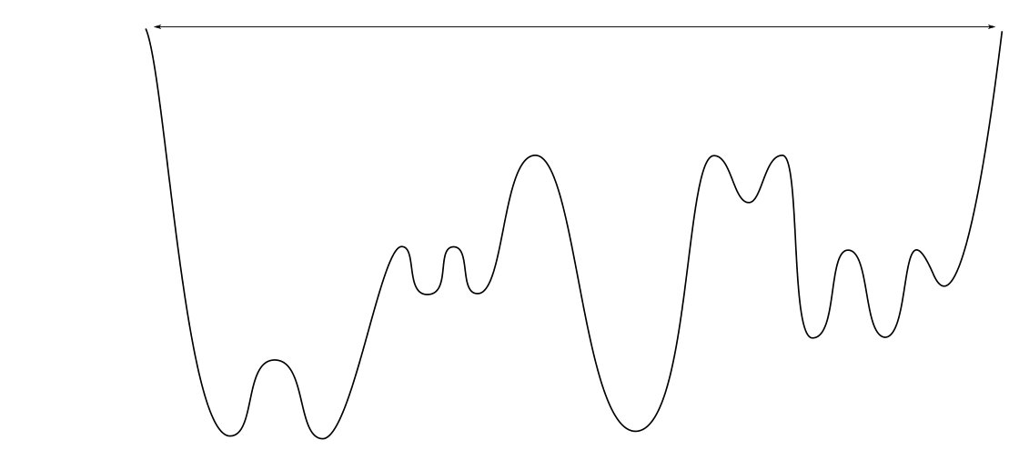 Figure 2
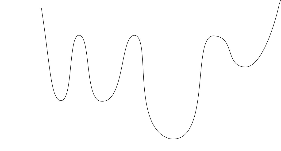 Figure 3
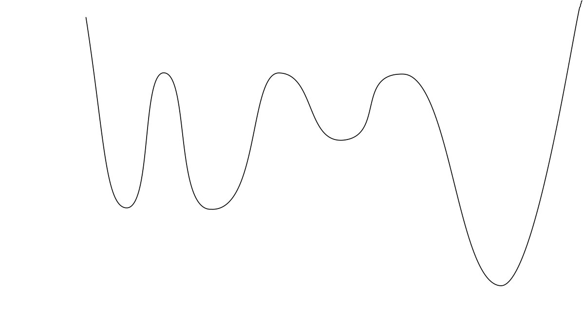 Figure 4
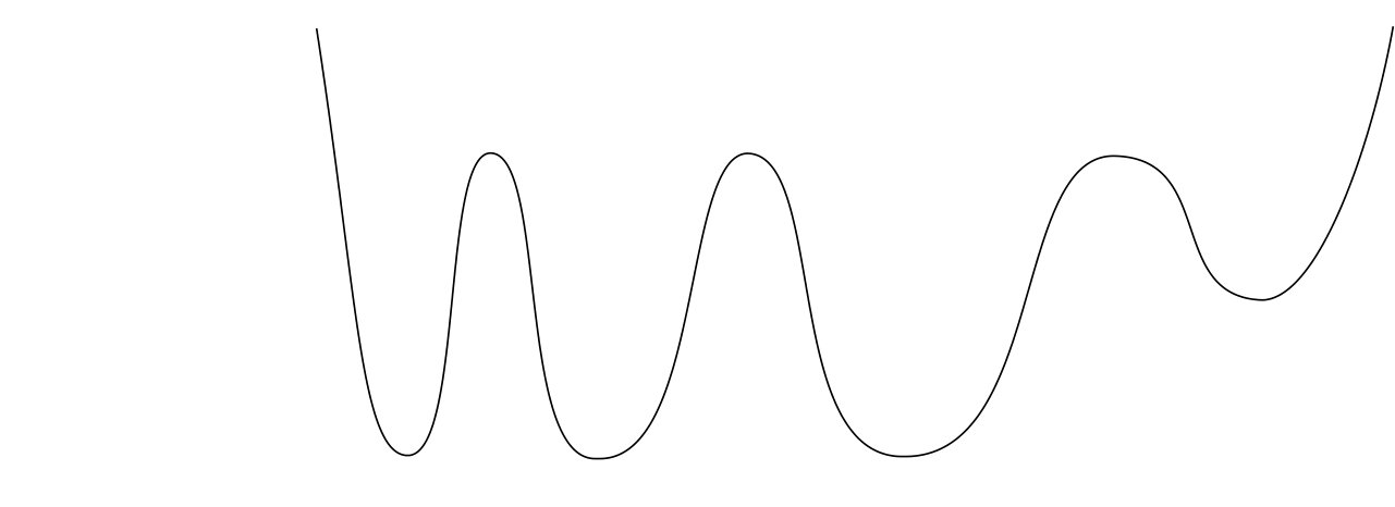 Figure 5
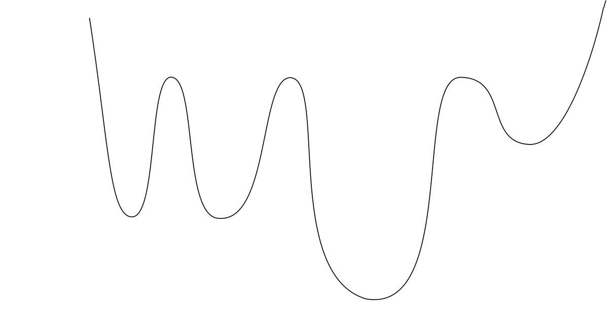 Figure 6
 Figure 7
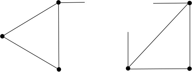 Figure 8
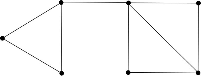 Figure 9
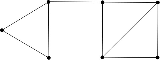 Figure 10
 Figure 11
 Figure 12
 Figure 13
 Figure 14