Robust inference for threshold regression models
Javier Hidalgo, Jungyoon Lee, Myung Hwan Seo

TL;DR
This paper develops robust inference methods for threshold regression models that are valid whether the threshold point has a kink or a jump, addressing irregularities in the likelihood function and providing practical confidence interval procedures.
Contribution
It introduces a unified inference framework for threshold models that works under both continuity and discontinuity assumptions, handling irregularities in the likelihood Hessian.
Findings
The proposed method achieves correct coverage probabilities in simulations.
The scale parameter can be consistently estimated using a kernel method.
Bootstrap test inversion provides reliable confidence intervals in finite samples.
Abstract
This paper is concerned with inference in threshold regression models when the practitioners do not know whether at the threshold point the true specification has a kink or a jump. We nest previous works that assume either continuity or discontinuity at the threshold point and develop robust inference methods on the parameters of the model, which are valid under both specifications. In particular, we found that the parameter values under the kink restriction are irregular points of the Hessian matrix of the expected Gaussian quasi-likelihood. This irregularity destroys the asymptotic normality and induces the non-standard cube root convergence rate for the threshold estimate. However, it also enables us to obtain the same asymptotic distribution as in Hansen (2000) for the quasi-likelihood ratio statistic for the unknown threshold up to an unknown scale parameter. We show that this…
Click any figure to enlarge with its caption.
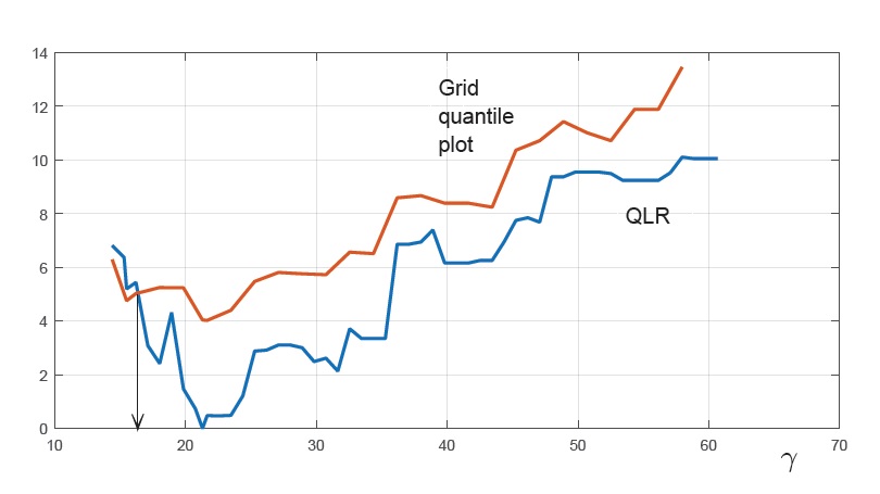 Figure 1
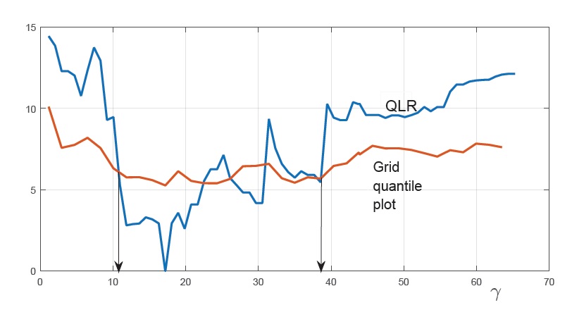 Figure 2
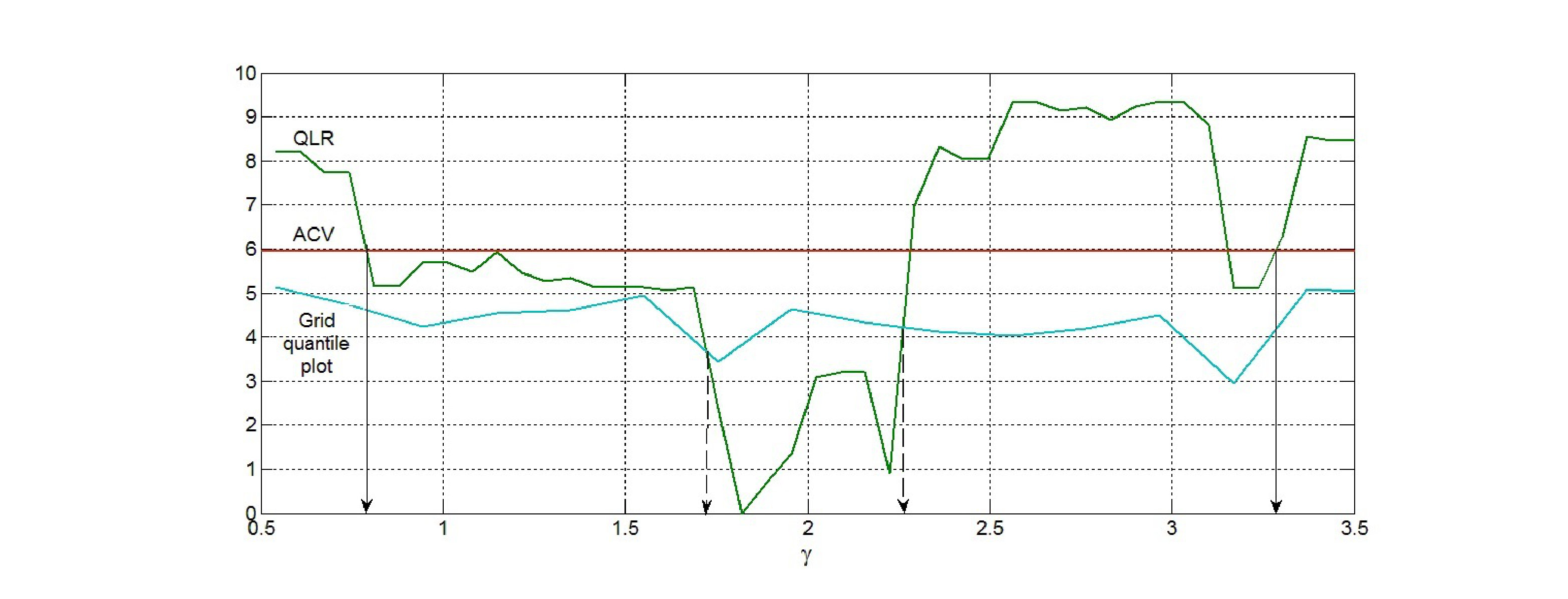 Figure 1
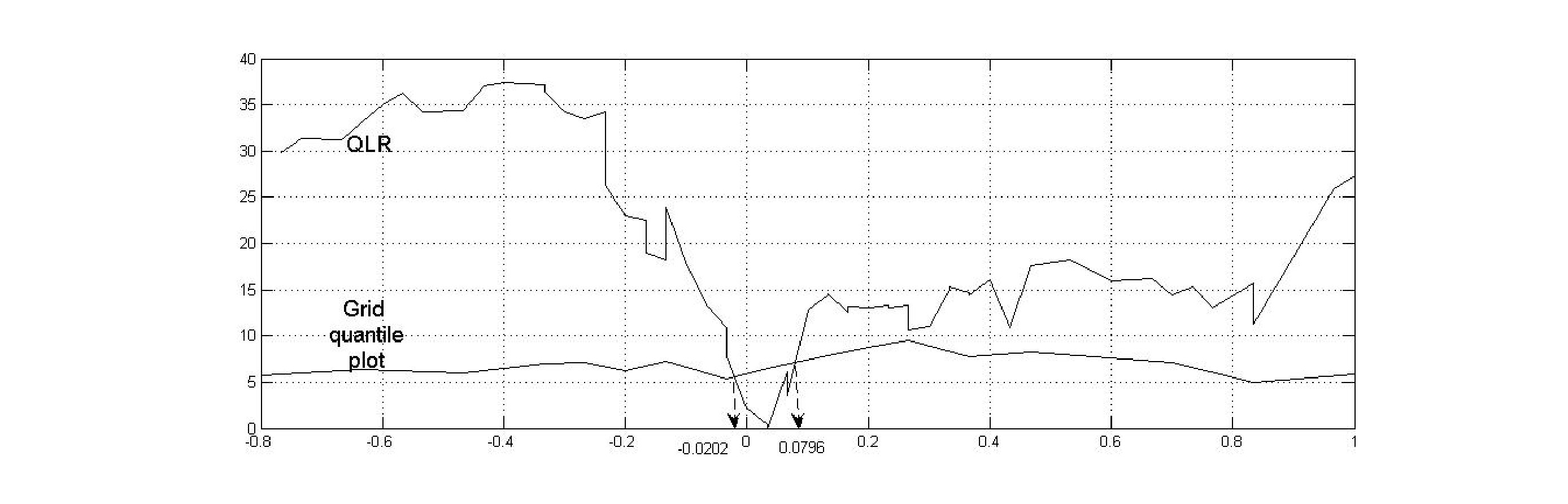 Figure 2
| Size | Coverage Probability | |||||||||||
|---|---|---|---|---|---|---|---|---|---|---|---|---|
| median of (2) | median of (2) | third quart. of (2.674) | ||||||||||
| \ | 100 | 250 | 500 | \ | 100 | 250 | 500 | 100 | 250 | 500 | ||
| 1/4 | Asym | 0.01 | 0.095 | 0.059 | 0.044 | 0.9 | 0.733 | 0.770 | 0.774 | 0.811 | 0.834 | 0.844 |
| 0.05 | 0.195 | 0.153 | 0.130 | 0.95 | 0.818 | 0.832 | 0.857 | 0.870 | 0.895 | 0.914 | ||
| 0.1 | 0.290 | 0.242 | 0.200 | 0.99 | 0.916 | 0.938 | 0.950 | 0.953 | 0.971 | 0.980 | ||
| B/rap | 0.01 | 0.003 | 0.015 | 0.009 | 0.9 | 0.756 | 0.810 | 0.840 | 0.783 | 0.826 | 0.852 | |
| 0.05 | 0.052 | 0.055 | 0.037 | 0.95 | 0.833 | 0.880 | 0.910 | 0.859 | 0.892 | 0.915 | ||
| 0.1 | 0.106 | 0.095 | 0.083 | 0.99 | 0.928 | 0.959 | 0.969 | 0.935 | 0.965 | 0.980 | ||
| 1/8 | Asym | 0.01 | 0.068 | 0.037 | 0.029 | 0.9 | 0.79 | 0.837 | 0.897 | 0.817 | 0.835 | 0.872 |
| 0.05 | 0.164 | 0.092 | 0.077 | 0.95 | 0.856 | 0.898 | 0.923 | 0.873 | 0.91 | 0.914 | ||
| 0.1 | 0.214 | 0.15 | 0.129 | 0.99 | 0.933 | 0.961 | 0.975 | 0.949 | 0.964 | 0.972 | ||
| B/rap | 0.01 | 0.006 | 0.009 | 0.008 | 0.9 | 0.791 | 0.846 | 0.881 | 0.792 | 0.827 | 0.871 | |
| 0.05 | 0.046 | 0.052 | 0.049 | 0.95 | 0.858 | 0.907 | 0.93 | 0.859 | 0.9 | 0.917 | ||
| 0.1 | 0.099 | 0.095 | 0.105 | 0.99 | 0.936 | 0.968 | 0.98 | 0.938 | 0.963 | 0.972 | ||
| Size | Coverage Probability | |||||||||||
|---|---|---|---|---|---|---|---|---|---|---|---|---|
| median of (2) | median of (2) | third quart. of (2.674) | ||||||||||
| \ | 100 | 250 | 500 | \ | 100 | 250 | 500 | 100 | 250 | 500 | ||
| 1/4 | Asym | 0.01 | 0.185 | 0.145 | 0.155 | 0.9 | 0.608 | 0.612 | 0.658 | 0.740 | 0.730 | 0.725 |
| 0.05 | 0.344 | 0.293 | 0.268 | 0.95 | 0.687 | 0.707 | 0.742 | 0.813 | 0.817 | 0.827 | ||
| 0.1 | 0.437 | 0.379 | 0.365 | 0.99 | 0.831 | 0.851 | 0.859 | 0.905 | 0.924 | 0.926 | ||
| B/rap | 0.01 | 0.022 | 0.013 | 0.021 | 0.9 | 0.770 | 0.836 | 0.866 | 0.868 | 0.882 | 0.878 | |
| 0.05 | 0.101 | 0.066 | 0.071 | 0.95 | 0.853 | 0.894 | 0.924 | 0.932 | 0.943 | 0.943 | ||
| 0.1 | 0.203 | 0.126 | 0.133 | 0.99 | 0.946 | 0.972 | 0.982 | 0.975 | 0.984 | 0.980 | ||
| 1/8 | Asym | 0.01 | 0.155 | 0.098 | 0.079 | 0.9 | 0.661 | 0.72 | 0.786 | 0.771 | 0.779 | 0.791 |
| 0.05 | 0.285 | 0.207 | 0.158 | 0.95 | 0.745 | 0.802 | 0.852 | 0.852 | 0.844 | 0.855 | ||
| 0.1 | 0.368 | 0.275 | 0.224 | 0.99 | 0.86 | 0.886 | 0.921 | 0.925 | 0.941 | 0.938 | ||
| B/rap | 0.01 | 0.029 | 0.009 | 0.017 | 0.9 | 0.797 | 0.871 | 0.904 | 0.886 | 0.891 | 0.888 | |
| 0.05 | 0.093 | 0.073 | 0.065 | 0.95 | 0.878 | 0.917 | 0.945 | 0.936 | 0.946 | 0.943 | ||
| 0.1 | 0.171 | 0.113 | 0.109 | 0.99 | 0.95 | 0.981 | 0.99 | 0.984 | 0.984 | 0.98 | ||
| Size | Coverage Probability | |||||||||||
|---|---|---|---|---|---|---|---|---|---|---|---|---|
| median of | median of | third quart. of | ||||||||||
| \ | 100 | 250 | 500 | \ | 100 | 250 | 500 | 100 | 250 | 500 | ||
| C | Asym | 0.01 | 0.123 | 0.028 | 0.005 | 0.9 | 0.802 | 0.946 | 0.975 | 0.749 | 0.925 | 0.972 |
| 0.05 | 0.168 | 0.043 | 0.015 | 0.95 | 0.84 | 0.965 | 0.983 | 0.784 | 0.945 | 0.98 | ||
| 0.1 | 0.200 | 0.056 | 0.024 | 0.99 | 0.892 | 0.982 | 0.992 | 0.852 | 0.966 | 0.99 | ||
| B/rap | 0.01 | 0.027 | 0.014 | 0.012 | 0.9 | 0.768 | 0.854 | 0.805 | 0.828 | 0.894 | 0.877 | |
| 0.05 | 0.091 | 0.054 | 0.052 | 0.95 | 0.817 | 0.918 | 0.889 | 0.88 | 0.949 | 0.943 | ||
| 0.1 | 0.153 | 0.108 | 0.104 | 0.99 | 0.905 | 0.979 | 0.975 | 0.954 | 0.981 | 0.984 | ||
| Size | Coverage Probability | |||||||||||
|---|---|---|---|---|---|---|---|---|---|---|---|---|
| median of (2) | median of (2) | third quart. of (2.674) | ||||||||||
| \ | 100 | 250 | 500 | \ | 100 | 250 | 500 | 100 | 250 | 500 | ||
| Asym | 0.01 | 0.0033 | 0.0032 | 0.002 | 0.9 | 0.969 | 0.976 | 0.971 | 0.969 | 0.979 | 0.975 | |
| (=0.7906) | 0.05 | 0.0133 | 0.0109 | 0.0093 | 0.95 | 0.987 | 0.988 | 0.987 | 0.98 | 0.991 | 0.986 | |
| 0.1 | 0.0266 | 0.0219 | 0.0203 | 0.99 | 0.999 | 0.998 | 0.998 | 0.998 | 0.999 | 0.997 | ||
| B/rap | 0.01 | 0.0104 | 0.0173 | 0.0114 | 0.9 | 0.837 | 0.859 | 0.836 | 0.839 | 0.848 | 0.843 | |
| 0.05 | 0.0691 | 0.0713 | 0.0674 | 0.95 | 0.87 | 0.901 | 0.868 | 0.87 | 0.883 | 0.875 | ||
| 0.1 | 0.1353 | 0.1358 | 0.1276 | 0.99 | 0.935 | 0.936 | 0.925 | 0.926 | 0.933 | 0.928 | ||
| 0.25 | Asym | 0.01 | 0.016 | 0.0074 | 0.0075 | 0.9 | 0.88 | 0.909 | 0.93 | 0.879 | 0.925 | 0.931 |
| 0.05 | 0.0599 | 0.0402 | 0.0322 | 0.95 | 0.938 | 0.95 | 0.972 | 0.927 | 0.958 | 0.961 | ||
| 0.1 | 0.1102 | 0.076 | 0.0648 | 0.99 | 0.985 | 0.992 | 0.993 | 0.982 | 0.994 | 0.984 | ||
| B/rap | 0.01 | 0.0146 | 0.0075 | 0.0121 | 0.9 | 0.873 | 0.876 | 0.894 | 0.851 | 0.896 | 0.897 | |
| 0.05 | 0.0585 | 0.0518 | 0.0563 | 0.95 | 0.934 | 0.93 | 0.939 | 0.916 | 0.949 | 0.943 | ||
| 0.1 | 0.1123 | 0.1024 | 0.1117 | 0.99 | 0.984 | 0.986 | 0.992 | 0.975 | 0.987 | 0.981 | ||
Peer Reviews
No public reviews on file for this paper yet. If you reviewed it on a platform where reviews are public (OpenReview, ICLR, NeurIPS, ICML), you can paste yours below so the community can read it here.
Videos
No videos yet. Explain this paper in a talk, walkthrough, or lecture? Add one.
Robust Inference for Threshold Regression Models††thanks: We thank anonymous referees and an Associate Editor for their constructive comments. M. Seo
gratefully acknowledges the support from Promising-Pioneering Researcher Program through Seoul National University (SNU) and from the Ministry of Education of the Republic of Korea and the National Research Foundation of Korea (NRF-0405-20180026).
Javier Hidalgo
London School of Economics
Jungyoon Lee
Royal Holloway, University London
Myung Hwan Seo
Seoul National University
Abstract
This paper is concerned with inference in threshold regression models when the practitioners do not know whether at the threshold point the true specification has a kink or a jump. We nest previous works that assume either continuity or discontinuity at the threshold point and develop robust inference methods on the parameters of the model, which are valid under both specifications. In particular, we found that the parameter values under the kink restriction are irregular points of the Hessian matrix of the expected Gaussian quasi-likelihood. This irregularity destroys the asymptotic normality and induces the nonstandard cube root convergence rate for the threshold estimate. However, it also enables us to obtain the same asymptotic distribution as in Hansen (2000) for the quasi-likelihood ratio statistic for the unknown threshold up to an unknown scale parameter. We show that this scale parameter can be consistently estimated by a kernel method as long as no higher order kernel is used. Furthermore, we propose to construct confidence intervals for the unknown threshold by bootstrap test inversion, also known as grid bootstrap. Finite sample performances of the grid bootstrap confidence intervals are examined through Monte Carlo simulations. We also implement our procedure to an economic empirical application.
JEL Classification: C12, C13, C24.
Key words: Change Point, Kink, Grid Bootstrap, Cube Root.
1 INTRODUCTION
This paper examines robust inference in threshold models without a priori knowledge on whether the model is or not continuous at the threshold point. Since its introduction, threshold models have gained a lot of attention in econometrics, statistics and other fields, see Tong (1990) and Hansen among others. In the time series context, their popularity is due to the fact that they are capable to explain nonlinear features present in many data such as chaos, cycles, irreversibility among others. In addition they have proved to have superior forecast performance in times of recession, see Tiao and Tsay .
We nest previous works that assume either continuity or discontinuity at the threshold point and develop robust inference methods on the parameters of the model, which are valid under both specifications When looking at inferences regarding these type of models, the literature has explicitly assumed that either the threshold regression model is continuous and kinked or it is discontinuous at the threshold point. For instance, Chan (1993) and Hansen have focused on inference when the model is discontinuous at the threshold point, whereas Chan and Tsay Hansen and Feder (1975a) have focused on inference in kink models. However, there is no a priori reason to believe that the model is or it is not continuous. The main motivation to have a “unified” or robust inference theory for these models is that their statistical properties are very different whether one estimates the model under the restriction of continuity or not. In particular, the estimates of the parameters of the model are all square root -consistent and asymptotically normal when the model is estimated under the (true) assumption of continuity, but under discontinuity the least squares estimator of is super consistent, asymptotically independent of the slope parameter estimates, and non-Gaussian. So, it is worthwhile to obtain some statistical properties of estimates of the parameters in a model that nests continuous and discontinuous frameworks.
We show an interesting property that the estimator of the threshold parameter fails to be root- consistent, contrary to what one might expect, if the model is continuous but the true restriction is not imposed in the estimation procedure. More specifically, we show that the rate of convergence of the estimate of the threshold point becomes in contrast to , which was first obtained by Feder and in the time series context by Chan and Tsay by imposing the (true) constraint of a kink in its estimation. The asymptotic distribution of the threshold estimator is no longer normal but the “” of some Gaussian process. On the other hand, we find that the unconstrained estimator of the slope parameters is asymptotically independent of the estimator of the threshold point, contrary to the findings in previous works. The asymptotic independence is also the case under the jump models of Chan or Hansen but not under the constrained estimation of Feder’s (1975) or Chan and Tsay’s (1998) kink models. This finding is interesting and new, when compared to standard results in regression models, where it is known that the consequence of not using the (true) restrictions is inefficiency but otherwise the asymptotic distribution is still Gaussian and the rate of convergence is the same. So, we conclude that the statistical inference for threshold regression models hinges too much on the unverified assumption of kink versus jump.
Our preceding discussion motivates us to develop a robust inference in the threshold regression model. To that end, we first show that a quasi-likelihood ratio statistic for the location of the threshold has the same asymptotic distribution up to a scale constant that depends on whether the true regression model has a kink or a jump. Second, we present an estimator for the scale factor based on the ratio of two kernel Nadaraya-Watson estimators. The consistency of this estimator is standard under the jump model but non-standard under the kink model because both its numerator and denominator converge to zero in probability. However, we prove that, similar to L’Hopital rule, the ratio of the two degenerating terms still converges in probability to the correct scale factor under the interesting requirement that higher-order kernels should not be used. Third, we show that the asymptotic distribution of the unconstrained estimator of the slope parameters when the model has a kink is identical to the one under the jump specification, which results from the asymptotic independence between the estimators of the slope and threshold parameters. This is not the case if the (correct) kink assumption were employed in the estimation of the parameters.
The last goal of this paper is to present valid bootstrap schemes for the construction of confidence sets for the threshold location. The motivation comes from the fact that sometimes the asymptotic critical values appear to be a poor approximation to the finite-sample ones, as documented by Hansen and also in our Section 5 among others. In addition, the first-order validity of the bootstrap is of theoretical interest and it has not been established even under the Hansen’s shrinking jump design. The interest stems from two sets of findings in the literature regarding the failure of bootstrap for non-standard estimators: firstly with cube-root estimators such as the maximum score estimator, and secondly with super-consistent estimators such as the estimator of autoregressive coefficients of unit root processes and the threshold estimator under Chan’s (1993) model, see Abrevaya and Huang , Seijo and Sen , and Yu , just to name a few. Note that the unconstrained estimator of the threshold belongs to the cube-root class under the kink model and to the super-consistent class under the jump models. Unlike failures of bootstrap in the cases listed above, we show that the proposed bootstrap statistics, which build on the wild bootstrap, correctly approximate the sampling distribution of the scaled quasi-likelihood ratio statistic in our settings. This contrast is perhaps due to the fact that the nuisance parameter in the asymptotic distribution under the non-shrinking model is infinite-dimensional while the ones in our continuous and shrinking specifications are finite-dimensional scaling terms. Furthermore, we propose bootstrap test inversion confidence interval for the threshold, also known as the grid bootstrap in Hansen , to enhance the finite-sample coverage probability.
We then present results of a small Monte Carlo experiment, which report good finite-sample performance of our bootstrap procedure for inference on the threshold location. In our empirical application, we apply our robust inferential method to the time series data on real GDP growth and debt-to-GDP ratio of a number of countries. Numerous works had fitted jump threshold models to a variety of of datasets, see e.g. Caner, Grennes, and Koehler-Geib , Cecchetti, Mohanty, and Zampolli , and Lee et al. , while Hansen had fitted kink threshold model to the US time series data. As there is little guidance from economic theory on suitability of jump or kink models, we advocate the use of our robust inference, and find substantial heterogeneity across countries in not just the estimated model parameters but also in the presence and location of threshold effect.
In Section 2 we introduce the model and present a set of regularity assumptions and describe how to estimate the parameters of the model. In particular, we examine the properties of the least squares estimator of the parameters when the model is continuous but we estimate them without this knowledge. In Section 3 we then develop robust inferential methods for model parameters that are valid under both continuous and discontinuous settings, despite the slower rate of convergence for the estimate of the threshold under the kink specification. We then present in Section 4 a bootstrap algorithm for inference on the model parameters, establishing their validity. Section 5 presents results of a small Monte Carlo study, followed by Section 6, which contains the empirical application. Section 7 concludes. This paper has an appendix that contains some of the proofs and an online supplement that presents the remaining proofs, technical lemmas, and more numerical results for Sections 5 and 6.
2 MODEL AND ESTIMATORS
We shall consider the following threshold regression model
[TABLE]
where denotes the indicator function and is a -dimensional vector of regressors. The parameter is referred to as a threshold point, taking values in a compact parameter space , which is a subset of the interior on the domain of the threshold variable . It is worth mentioning that all our results hold true also when , which is the case with structural break models. However, we have opted not to include this scenario for the sake of clarity and notational simplicity.
We assume that is an element of the regressor vector and denote
[TABLE]
where is partitioned to match the dimensionality of . Also we shall abbreviate and , so that we can write as
[TABLE]
Before stating some regularity assumptions on the model, we need to introduce some extra notation. Let denote the density function of , which we assume to exist, and , the conditional variance function of error term, while denotes the unconditional variance. Denote matrices , and let and . As usual the “[math]” subscript on a parameter indicates its true unknown value. Finally, let and with .
Assumption Z**.**
Let be a strictly stationary, ergodic sequence of random variables such that their -mixing coefficients satisfy and , where is the filtration up to time . Furthermore, , , and for some .
Assumption Q**.**
The functions , V\left(\gamma\right)\and are continuous at . For all , the functions , E\big{(}x_{t}x_{t}^{\prime}\mathbf{1}\left\{q_{t}\leq\gamma\right\}\big{)} and are positive and continuous, and the functions ,\ E\big{(}|x_{t}|^{4}|q_{t}=\gamma\big{)} and E\big{(}|x_{t}\varepsilon_{t}|^{4}|q_{t}=\gamma\big{)} are bounded by some .
Assumptions **Z **and Q are commonly imposed on the distribution of , see e.g. Hansen , so his comments apply here. As discussed therein, the self-exciting threshold autoregressive model of Tong satisfies Assumption Z. The condition for is written in terms of as the other elements in are fixed given . While we allow conditional heteroscedasticity of a general form, Assumption Q requires continuity of the conditional variance function at .
2.1 Estimators
We estimate by the (non-linear) least squares estimator (LSE), that is,
[TABLE]
where is a compact set in and
[TABLE]
which is a step function in at ’s. For its computation, we shall employ a step-wise algorithm. To that end, one could employ the grid search algorithm on to find . Define the concentrated sum of squared residuals
[TABLE]
where
[TABLE]
is the LSE of for a given . Then, our estimator of is , with
[TABLE]
Since the minimizer is given by an interval, it is common to let the estimator be the maximum. This is the unconstrained LSE and for comparison we also describe the continuity constrained least squares estimator (CLSE), which minimizes under Assumption C in the next section,
[TABLE]
This estimator was considered by Feder and later by Chan and Tsay or Hansen who have established the asymptotic normality of with the standard squared root consistency.
3 Robust Confidence Regions
This section presents our main results, namely how to perform robust inference in threshold models and in particular on the location of the threshold point. We begin with developing inference methods for the regression coefficients and the unknown threshold based on the LSE when the true regression model has a kink. Then, they are compared with other inference methods that are developed under different sampling schemes such as Hansen . In particular, we show that a judicious choice of statistics enables us to perform a robust inference in the sense that the same critical values can be employed for inference whether the model has a kink or a jump. That is, we do not need to know whether the model has a kink or a jump to make inference for the parameters and . As mentioned in the introduction the motivation comes from the rather surprising results given in Proposition 1 and Theorem 1 below.
First we state the kink model in terms of assumption.
Assumption C**.**
Assume that and
[TABLE]
Under Assumption C the model (2) is written as
[TABLE]
Feder (1975), Chan and Tsay (1998), and Hansen (2017) considered the estimation of the model (11) along with an auxiliary condition of to ensure the identification of the change-point . This is a model with a kink.
Then, the next proposition establishes the consistency and rates of convergence of the LSE defined in under Assumption C.
Proposition 1**.**
Under Assumptions C, Z and Q, we have that
[TABLE]
The results of Proposition 1 are surprising because the convergence rate of is slower than that of the CLSE , which is known to be as shown in the aforementioned works. That is, using the true restriction on the parameters leads to a faster rate of convergence of the estimator of , not just reducing its asymptotic variance as is often the case.
Next we present the asymptotic distribution of .
Theorem 1**.**
Let Assumptions C, Z and Q hold and and be two independent standard Brownian motions. Define . Then,
[TABLE]
where the two limit distributions are independent of each other.
The asymptotic independence is a consequence of the different convergence rates between the two sets of estimators and by similar arguments as in Chan , albeit the rate for being slower than that for in our case. The asymptotic independence does not hold for the CLSE and , which converge at the same rate as mentioned above and they are jointly asymptotically normal with a non-diagonal variance covariance matrix.
Theorem 1 suggests that Gonzalo and Wolf’s subsampling procedure would be correct if they had used the normalization instead of the incorrect one . On the other hand, it is worth mentioning that Seo and Linton considered the smoothed least squares estimator for the same setup. The convergence rate for their smoothed least squares estimator for was slower than our cube-root rate under their assumptions for the smoothing parameter.
Remark 1**.**
We now present a heuristic discussion to illustrate why the constrained and unconstrained estimators of have different rates of convergence and the unconstrained estimator belongs to the cube-root class explored by Kim and Pollard for the data and Seo and Otsu for more general setups. For simplicity of illustration, we begin with a simplified model, where , , is fixed at , and thus . In addition we shall assume and thus by (10) without loss of generality since we can always rename the variable as . It is well known that the rates of convergence of an M-estimator is governed by the local behavior of its criterion function around the true value provided that the estimator is consistent. Then the convergence rate of LSE is determined by the stochastic expansion of
[TABLE]
in small neighborhoods of and . Consider . The case of is handled similarly. Then, as and ,
[TABLE]
because for some positive constant ,
[TABLE]
due to Assumption Q. This cubic approximation at is non-standard and invalidates the asymptotic normality of , which builds on the quadratic approximation.111This also shows that the asymptotic variance formula in Gonzalo and Wolf’s (2005) Theorem A.1 and Remark A.1 is not properly defined due to the degeneracy of , where is the second derivative matrix of the expected criterion function that is evaluated under the continuity restriction. Similarly,
[TABLE]
Thus, the last two displayed expressions suggest that
[TABLE]
as these rates of convergence balance the speeds at which the bias and standard deviation of converge to zero. In comparison, the CLSE is ruled by
[TABLE]
due to the continuity constraint (10), for which we observe the quadratic expansion
[TABLE]
This yields that
[TABLE]
which coincides with the rates of convergence that both Feder a, b) and Chan and Tsay obtained.
An intuitive explanation for the preceding Proposition, Theorem, and Remark is to appeal to “misspecification”. Although the unconstrained model (1) encompasses both continuous and discontinuous models, the estimated regression function is almost surely discontinuous, since the probability that the LSE fulfills the continuity restriction is zero.
3.1 Inference on Regression Coefficient
Theorem 1 in Section 3.1, Lemma A.12 of Hansen and Theorem 2 of Chan report the same asymptotic distribution for namely , which is asymptotically independent of . Thus, the inference for is uniform under any widely used sampling scheme with strongly identified , provided that the respective sample moments
[TABLE]
where , are consistent under each data generating process. This is the case due to the uniform law of large numbers, which only requires consistency of .
It is worthwhile to mention that this “oracle” property of does not hold true for the CLSE , whose asymptotic distribution is affected by that of , as was first noticed and shown by Feder and later extended to time series data by Chan and Tsay .
3.2 Inference on Threshold
The main purpose of this section is to develop a method to construct confidence regions for that is valid regardless of whether the regression model has a kink or a jump at the true value of . Conventionally, inference on has been done after assuming either that the model has a kink or that it has a jump, i.e. the practitioner chooses between jump or kink models before estimating the threshold point. More specifically, if we decide that the model has a jump, then one follows e.g. Hansen , whereas if one has chosen the kink model then one needs to employ the asymptotic normal inference as in Feder and others. One of our findings is that Hansen results are not valid if the model had a kink and likewise Feder’s results are not valid if the model had a jump.
Thus, this section develops robust confidence regions that are valid regardless which of the two models is the true specification. To ease reference, we recall Hansen’s (2000) diminishing jump specification:
Assumption J**.**
For some and , and d^{\prime}Vd\and are positive for all .
When is greater than or equal to , is too small to consistently estimate , and such case is excluded. And we suppress the dependence of on the sample size to simplify the notation.
To develop robust confidence sets, we need to find a statistic whose asymptotic distribution is invariant to the true parameter value, that is, a statistic whose asymptotic distribution does not change suddenly under Assumption C. We begin by introducing a Gaussian quasi-likelihood ratio statistic based on the unconstrained model . Specifically, let
[TABLE]
where is defined in .
We now derive the following asymptotic distribution for , which contrasts with the asymptotic distribution obtained by Hansen under Assumption J.
Proposition 2**.**
Suppose that Assumptions C, Z and Q hold. Then, as ,
[TABLE]
where
[TABLE]
In comparison, we recall Hansen’s (2000) results that
[TABLE]
where
[TABLE]
and that the distribution function of is given by .
The results of our Proposition 2 and that in indicate that the only difference between the limit distributions of under the kink and jump specifications is the scaling factor. This is the case despite the fact the estimator exhibits different rates of convergence across the two settings.
Next, we propose an estimator of the unknown scaling of that converges in probability to under Assumption J, while it converges to under Assumption C, thus adapting to the unknown true scaling in each situation. We begin with a natural estimator of , which is a ratio of two Nadaraya-Watson estimators of the conditional expectations. That is,
[TABLE]
where and are, respectively, the kernel function and bandwidth parameter and ’s are the least squares residuals. The consistency of to is standard, as argued in Hansen .
However, it is not trivial to establish that when the true model has a kink at because both numerator and denominator degenerates asymptotically in Assumption C. It turns out that we need to impose some unconventional restrictions on the kernel function and the bandwidth . Specifically, we assume
Assumption K**.**
Assume the following for and
is symmetric and for and .
is twice continuously differentiable with the first derivative and for all u\such that as .
, where the characteristic function satisfies that is integrable.
as .
It is clear that the Epanechnikov and the Gaussian kernel functions satisfy , and . One important observation is that rules out higher-order kernels by assuming . The consequence of dropping the assumption that is discussed in detail in Remark 2 that follows the next proposition.
Proposition 3**.**
Suppose Assumptions Z, Q and K hold true. Then, under Assumption C
[TABLE]
while under Assumption J.
Remark 2**.**
We now comment on the consequence of dropping the assumption that . If we allowed for higher-order kernels, that is and but , would not be consistent. Indeed, Proposition 3 and Lemma 2 in the Appendix indicate that, without loss of generality for and , converges in probability to
[TABLE]
where g_{r}\left(q\right)=E\left(x_{t2}^{r}\varepsilon_{t}^{2}\mid q_{t}=q\right)\and . This is the case because dropping in the assumption of and letting , the numerator in will be
[TABLE]
whereas the denominator in becomes
[TABLE]
So that, unless , we obtain that (similar to the L’Hopital rule):
[TABLE]
and hence would not be a consistent estimator of the scale factor .
We can construct the percent confidence set of by
[TABLE]
As we have already argued, this confidence set is valid under both scenarios, as the next theorem shows.
Theorem 2**.**
Let Assumption K, Z and Q hold true and suppose that either Assumption C or J hold. Then, for any ,
[TABLE]
4 BOOTSTRAP
This section develops a bootstrap-based test inversion confidence interval for the unknown threshold parameter , which is valid under Assumption C as well as under Assumption J. We do not discuss the bootstrap for in detail but note that the bootstrap for the linear regression can be employed,222This excludes the case where is not strongly identified in the sense that with . This case has not been explored except when , see e.g. Hansen (1996) and it is an interesting future research area. see e.g. Shao and Tu , since we can treat as for the inference on due to the arguments leading to the asymptotic independence between and .
We propose using the bootstrap test inversion method, also known as the grid bootstrap, of Dümbgen to build confidence intervals for the parameter , see also Carpenter and Hansen . Such a test inversion bootstrap confidence interval (BCI) is known to have certain optimality properties as in e.g. Brown, Casella and Hwang from the Bayesian perspective. Mikusheva showed that test inversion BCI attains correct coverage probability uniformly over the parameter space for the sum of coefficients in autoregressive models, despite the behavior of the estimator not being uniform over the parameter space.
For a given confidence level , one can exploit the duality between hypothesis testing and confidence interval by inverting tests to obtain a confidence region
[TABLE]
where is the bootstrap estimate of the th quantile of the statistic when . In other words, it denotes the bootstrap critical value of level () testing for . In practice, one would estimate over a grid of and use some smoothing method such as linear interpolation or kernel averaging to obtain a smoothed bootstrap quantile function over a range of . The region is known as -level grid bootstrap confidence interval (BCI) of in the terminology of Hansen .
Figure 1 illustrates how this confidence interval can be obtained in practice. The line is the linear interpolation of the rescaled statistic over the grid of at 50 points. The ACV line is the asymptotic critical value of Hansen . The true value of was . We estimated bootstrap quantile function (described in the sequel) at 17 grid points and present the interpolated line as Grid quantile plot. The vertical arrow at intersections between and ACV yield the asymptotic confidence interval (ACI), while the vertical broken arrows indicate grid BCI based on the bootstrap.
Now, we describe the bootstrap procedure for the grid bootstrap. We repeat the following procedure for each values of .
4.1 Bootstrap Algorithm for each
STEP 1
Obtain LSE by minimizing and compute the LSE residuals
[TABLE]
STEP 2
Generate as zero mean random variables with unit variance and finite fourth moments, and compute
[TABLE]
STEP 3
Obtain the least squares estimate using and
[TABLE]
STEP 4
Compute the bootstrap analogues of and as
[TABLE]
and
[TABLE]
where is defined analogously as in (6) by replacing with .
STEP 5
Compute the bootstrap 100-th quantile from the empirical distribution of by repeating STEPs 2-4.
Next, we derive the convergences of the bootstrap LSE and for both continuous and discontinuous setups and show the consistency of the bootstrap statistic . These results then yield the validity of the bootstrap test inversion confidence set following the same arguments in the proof of Theorem 2.
As usual, the superscript “∗” indicates the bootstrap quantities and convergences of bootstrap statistics conditional on the original data. As in Shao and Tu (1995), the notation “ *in Probability” *signifies the the convergence in Probability of the random distribution functions of the bootstrap statistics in terms of the uniform metric and means that in Probability.
Theorem 3**.**
*Suppose that Assumptions Z and Q hold true.
Under Assumption C, and are asymptotically independent and (in probability)*
[TABLE]
* Under Assumption J, and are asymptotically independent and (in probability)*
[TABLE]
Our results can be compared with those already obtained in the literature regarding the validity of bootstrap for non-standard estimators. First, our consistency result seems to contradict Seijo and Sen’s result on the inconsistency of a residual-based bootstrap and the nonparametric bootstrap (with data) for the case where , see also Yu . The reason behind such contradictory conclusions lies in the observation that our setup differs from theirs in an important and vital way: they consider the case of a fixed size of the break whereas we consider the situation that decreases with the sample size. Thus, their limiting distribution depends on the whole conditional distribution of given in a complicated manner, whereas ours contains only an unknown scaling factor.
It is worth mentioning that the centering term for is , which reflects the fact that our resampling scheme imposes the hypothesized true value for the unknown threshold. This is important for the validity of our bootstrap since we do not impose the continuity restriction in our bootstrap resampling. By imposing the null value, our resampling scheme builds on -consistent estimates.
Next, the consistency of is established in the following proposition.
Proposition 4**.**
Suppose Assumptions Z, Q and K hold and either of Assumption J or Assumption C holds true. Then,
[TABLE]
A direct consequence of Theorem 3 and Proposition 4 is the following theorem.
Theorem 4**.**
Now, suppose either Assumption J or Assumption C hold true in addition to Assumptions Z, Q and K. Then, (in probability)
[TABLE]
5 Monte Carlo Experiment
We generate data based on the following 3 specifications, with settings A and B being jump models akin to that considered in Hansen (2000, Section 4.2) and setting C representing the kink case.
[TABLE]
The main difference in our data generating process from that of Hansen (2000) is the conditional heteroscedasticity in : we set where and were generated as mutually independent and normal random variables with unit variance. This leads to conditional heteroscedasticity of the form , in contrast to Hansen (2000) where was generated from . In setting A, we generated as draws from , independent of and , while we set We generate and the same for setting B. For both settings A and B, we try and , which correspond to the median and third quartile of , respectively. In setting C, we set and try or so that the threshold corresponds to the median or the third quartile of , respectively. For the grid used in estimation of , we discarded of extreme values of realized and used number of equidistant points.
We investigate finite-sample performance of testing and confidence regions for given in Sections 3 and 4. We first compare the Monte Carlo size of tests for the correct location of the threshold, based on the asymptotic theory of Hansen , which covers diminishing jump models, and our bootstrap method. We then investigate coverage probabilities of confidence intervals, constructed from either the asymptotic theory of Hansen , or test-inversion based on our bootstrap. Our method has the virtue of robustness across different settings, and the objective is to see how it works across the jump settings of A and B and the kink setting of C. In A and B, we try two sets of with : , and for reflecting Assumption J. In setting C, is fixed at in line with Assumption C.333Note that were the smallest and the largest values of tried in Hansen (2000), respectively. For the estimate of the scale factor for the statistic, Epanechnikov kernel and minimum-MSE bandwidth choice, given in Härdle and Linton , were deployed.
Columns 4-6 of Tables 1-3 present Monte Carlo size of test of when is the median of for nominal sizes for the three settings. We carried out 10,000 iterations, with one bootstrap per iteration, using the warp-speed method of Giacomini, Dimitris and White (2013). Using the asymptotic critical values delivers poor Monte Carlo sizes in settings A and B with substantial over-sizing, which is more severe in setting B. In contrast, the bootstrap test produces sizes that are close to the nominal ones, apart from in B, for both . For the asymptotic test, the size results are somewhat better when compared to in settings A and B, although the over-sizing remains severe even for in setting B as shown in Table 2. For the kink setting C, asymptotic test based on Hansen’s results produces sizes that become very small with increasing , while the bootstrap test leads to good size results for .
Columns 8-10 of Tables 1-3 report the coverage probabilities of confidence intervals for in the three settings, when is the median of , and columns 11-13 present the case when is the third quartile of , for confidence levels . Results are based on 1,000 iterations and in each iteration, we generated bootstrap quantile plots by interpolating bootstrap quantiles obtained at 10 equidistant points of the realized support of from 399 bootstraps, and found intersections with the sample plot formed by interpolating between number of equidistant points after discarding of extreme values of realized .
In settings A and B reported in Tables 1 and 2, the coverage probability results are better when is the third quartile of for both methods when . For , this is still the case, with the exception of bootstrap coverage probabilities in setting A, which are similar between the two values of . In setting A as shown in Table 1, the asymptotic and bootstrap methods perform similarly, reporting lower-than-nominal coverage probabilities which improve with larger . In setting B, the bootstrap method delivers substantially better coverage probabilities than the asymptotic confidence intervals based on Hansen , which remain substantially lower than the nominal level even for for . Such under-coverage of asymptotic confidence intervals for small was also reported in Hansen’s (2000) Table 2, for homoskedastic error case. The coverage probability results are better when compared to for both methods in setting B, especially so for asymptotic confidence intervals. In Hansen’s (2000) Table 2, coverage probability was also good for .
In setting C reported in Table 3, the asymptotic coverage probabilities becomes close to 1 for all values of for , while bootstrap coverage probabilities are satisfactory for . The bootstrap coverage probability is better when is the third quartile of compared to when it is the median.444In Table 4 in Online Appendix, we report Monte Carlo size and coverage probability results for when with fixed at and in setting A () with homoscedastic error. Fixed jump setup is not covered by Hansen (2000) or our bootstrap of Section 4, but nonetheless we investigate how the two methods perform in this setting for completeness.
6 EMPIRICAL APPLICATION: GROWTH AND DEBT
The so-called Reinhart-Rogoff hypothesis postulates that above some threshold (90 being their estimate of this threshold), higher debt-to-GDP ratio is associated with lower GDP growth rate. There have been numerous studies that utilize the threshold regression models to assess this hypothesis, including Hansen who fitted a kink model to a time series of US annual data, see Hansen for references on earlier studies which fitted jump models to various data sets. As there is little guidance from economic theory on the choice between kink and jump models in this setting, we advocate the use of our robust inference on the threshold and slope parameters of the model.
Hansen had fitted a kink model to US annual data on real GDP growth rate in year () and debt-to-GDP ratio from the previous year () for the period spanning 1792-2009 (), and estimated the threshold to be , while the slope parameters of were not significant. Before fitting the jump model to this data, we first tested for the presence of threshold effect using the testing procedure of Hansen (1996) with 1,000 bootstrap replications, and obtained -value of 0.047, rejecting the null hypothesis of no threshold effect. This is in contrast to the -value of 0.15 obtained by Hansen’s test for presence of threshold effect when imposing the kink model. Hansen had remained inconclusive on the presence of kink threshold effect, since the bootstrap method used there did not account for the time series nature of data and the high -value could have been due to modest power of the test.
The fitted jump model is given by:
[TABLE]
The sizes of the two regimes were 99 (below 17.2) and 109 (above 17.2). We obtained grid bootstrap confidence intervals for to be (10.5, 39) for 95 confidence level and (10.8, 38.6) for 90, based on 399 bootstrap iterations. Bootstrap quantiles were obtained at 38 grid points, which included , and equidistant points on the realized support of after discarding 7.5 of the largest and smallest values of in the sample.555There is currently no theoretical guide to the choice of the trimming parameter. Our choice of trimming out 7.5 was guided by Sweden’s estimated being the 12-th percentile of the in the data. Sensitivity check on changing choices of the trimming value is recommended. We find the points of intersection between the linearly interpolated bootstrap quantile line and the linear interpolation of sample test statistics for at grid points consisting of 73 equidistant points and , , as shown in Figure 2 for 90 confidence level.
As the estimated threshold under the jump model is noticeably small at 17.2, our estimated jump model which suggests insignificance of effect of on above the threshold does not necessarily contradict the Reinhart-Rogoff hypothesis. To see if this could be an indication of presence of further threshold points, we applied Hansen (1996)’s testing procedure for presence of threshold effect on the lower and upper subsamples with 1000 bootstraps and obtained -values of 0.025 and 0.016, respectively. Hence, we conclude that the US time series data should be fitted to a threshold regression model with multiple threshold points.
To see if such conclusion holds across different countries, we proceeded by first applying Hansen (1996)’s test for the presence of threshold effect on Reinhart and Rogoff’s (2010) data for countries with relatively long time spans without missing observations. For Australia() and the UK(), the -values with 1000 bootstraps were 0.795 and 0.98 so we conclude that there is no threshold effect for these countries in the relationship between the GDP growth and the debt-to-GDP ratio.
For data from Sweden for the period 1881-2009 (), the -value for Hansen (1996)’s test of presence of threshold effect with 1000 bootstraps for the whole sample is 0.048, while for the lower and upper regimes, divided by , they were 0.979 and 0.131, respectively. The estimated jump model is:
[TABLE]
with the lower regime having 61 observations and upper regime containing 68. The coefficient of debt-to-GDP ratio is not statistically significant.
The grid bootstrap confidence intervals for were (15.3, ) and (16.4, ) for 95 and 90 confidence levels. Shown in Figures 3 are linear interpolation of 90 bootstrap quantiles at 27 grid points with 399 bootstraps and linear interpolation of QLR test statistic at each of 54 grid points.
We conclude that there is substantial heterogeneity across countries in the relationship between the GDP growth and the debt-to-GDP ratio, not only in the values of model parameters, but also in the kinds of models that are suitable.
7 CONCLUSION
This paper has developed unified inferential procedures for the threshold regression model. The unconstrained least squares estimator of the regression coefficient turns out to enjoy the useful oracle property, which enables the standard asymptotic normal inference as in the linear regression model. On the other hand, we provide a judiciously constructed statistic, with which one can make inference of the unknown threshold without knowing the continuity of the threshold regression model. Asymptotically valid bootstrap inference is also proposed and shown to improve the finite sample performance of the asymptotic procedure.
An interesting future research area is extension to the nonparametric setting. For instance, see Card et al. (2008) and Pan (2015), who use the regression discontinuity methods 666Pan (2015, p.378) and a referee emphasize that this setting is not identical to the conventional regression discontinuity method (e.g. Angrist and Lavy (1999); Hahn et al. (2001)) due to the lack of knowledge on the precise location of the discontinuity. to test for the tipping phenomenon in racial segregation and gender segregation, respectively, or Landais (2014), who recommends testing for the location of the change-point as a validity check for the regression discontinuity design, even when the change-point is suggested by the institutional knowledge.
Appendix A PROOFS OF MAIN THEOREMS
Let us introduce some notation first. In what follows … denote generic positive finite constants, which may vary from line to line or expression to expression. Recall that , and , and introduce . Finally, we abbreviate by for any parameter .
All the technical lemmas are given in the online supplement to this paper.
A.1 Proof of Proposition 1
Without loss of generality we assume that and , so that \delta_{10}=0\and under Assumption C. By definition, we have that
[TABLE]
By standard algebra and denoting ,
[TABLE]
which implies, because of the orthogonality of the terms on the right of the last displayed expression, that
[TABLE]
where
[TABLE]
**Consistency. ** It suffices to show that for any , , there is such that for all , , which is implied by
[TABLE]
where for .
First implies that either and , or or . When holds true, it is clear that
[TABLE]
whereas when holds true, we have that
[TABLE]
because Assumption Q implies that , and are positive definite matrices uniformly in and if because we can always choose such that . We have that
[TABLE]
where . The motivation for the last displayed inequality comes from the fact that , say, implies that is a strictly positive and finite definite matrix which implies that for any vector ,
[TABLE]
So, and imply that
[TABLE]
On the other hand, Lemma 1 and the uniform law of large numbers, respectively, imply that
[TABLE]
where , and hence
[TABLE]
Thus because the left side of is bounded by
[TABLE]
using and .
**Convergence Rate. **We shall show next that for any there exist , , such that for we have that
[TABLE]
Since for any sequence and and for any functions and , it suffices to show that for each
[TABLE]
[TABLE]
To that end, we shall first examine
[TABLE]
where
[TABLE]
Recall that we have assumed that , as the case follows similarly.
First by standard arguments,
[TABLE]
by Lemma 1 and the Markov’s inequality. Observe that the latter inequality is independent of . Since , the probability in can be made arbitrary small for large or small , thus satisfying the condition . follows similarly as is the case for and thus it is omitted.
We next examine and for . Observing and the arguments that follow, defining
[TABLE]
it suffices to show and for and . To that end, because as , we obtain, since
[TABLE]
by Lemma 1 and Markov’s inequality. Notice that this bound is independent of . But by summability of , we conclude that holds true for by choosing large enough.
We now conclude the proof after we note that the left side of is bounded by
[TABLE]
using .
A.2 Proof of Theorem 1
Because the “” is a continuous mapping, see Kim and Pollard , and the convergence rates of and are obtained in Proposition 1, it suffices to examine the weak limit of
[TABLE]
over , where we assume as before for notational convenience and reparametrize and First, due to the uniform law of large numbers it follows that
[TABLE]
whereas Lemma 1 and the expansion of as in (30) imply that
[TABLE]
Therefore
[TABLE]
where
[TABLE]
The consequence of is then that the minimizer of is asymptotically equivalent to that of . Thus, it suffices to show the weak convergence of and and that
[TABLE]
are . The convergence of and its minimization is straightforward since it is a quadratic function of
Next, the first term of converges to uniformly in probability because Lemma 1, i.e. (47), implies the uniform law of large numbers and the Taylor series expansion up to the third order yields
[TABLE]
where . When , it follows similarly as in this case the derivative should be multiplied by , so that the limit becomes .
The second term in the definition of that is converges weakly to . To see this note that Lemma 1, i.e. (46), yields the tightness of the process as explained in Remark 3. For the finite dimensional convergence, we can verify the conditions for martingale difference sequence CLT (e.g. Hall and Heyde’s (1980) Theorem 3.2). In particular, we need to show that for ,
[TABLE]
For , note that as . For , apply the same argument for the first term in and an expansion similar to that in . We now characterize the covariance kernel. To that end, we note that if and have different signs then the cross product becomes zero and for , similarly as with , we have that
[TABLE]
The cases for g_{1}>g_{2}>0\or are similar and thus omitted.
Finally, the covariance between and vanishes for the same reasoning, yielding the independence between and and thus the asymptotic independence between and the threshold estimator .
A.3 Proof of Proposition 2
Due to the asymptotic independence between and in Theorem 1, see (29) in its proof, we have that
[TABLE]
which corresponds to in the proof of Theorem 1 due to the reparameterization . It also shows that
[TABLE]
Finally, the desired result follows from applying the change of variables because of the distributional equivalence (and ) and the fact that for any function .
A.4 Proof of Theorem 2
It is known that the distribution function of is , as in Hansen (2000). Thus, under Assumption C, Propositions 2 and 3 yield the conclusion, while under Assumption J, Theorem 2 of Hansen (2000) verified the conclusion.
A.5 Proof of Theorem 3
Recalling our definition of and in , we begin by showing their consistency and rate of convergence, which is given in Proposition 5.
We now discuss the asymptotic distribution of the bootstrap estimators. We begin with part . We assume to simplify notation. Because the “” is continuous as mentioned in Theorem 2, it suffices to examine the weak limit of
[TABLE]
where .
First, recall that and under Assumption C and note that Lemma 1 and Lemma 4 imply that, uniformly in ,
[TABLE]
Thus, the latter implies that
[TABLE]
where
[TABLE]
The consequence of is then that the minimizer of is asymptotically equivalent to that of . Thus, it suffices to show the weak convergence of and and that
[TABLE]
are . The convergence of and its minimization follows by standard arguments as it is a quadratic function of so that it suffices to examine and it minimum.
Turning to the second term in the definition of we show that it converges to weakly (in probability). To this end, note that Lemma 4’s, and the Remark 4 that follows, yields the tightness of the process as explained in Remark 3. For the finite dimensional convergence, it follows by standard arguments as
[TABLE]
which converges in probability to and the Lindeberg’s condition follows easily.
Part is also proved similarly and thus omitted for the sake of space.
A.6 Proof of Theorem 4
This is a direct consequence of Theorem 3 and Proposition 4 and the same arguments as the proof of Theorem 2.
Online Supplement to “Robust Inference in Threshold Regression Models”
by Javier Hidalgo, Jungyoon Lee, and Myung Hwan Seo
This supplement contains more numerical results for Section 5 and the remaining proofs of main theorems and supporting lemmas.
Appendix B-1 Table 4 for Monte Carlo study in Section 5
In Table 4, we report Monte Carlo size and coverage probability results for when with fixed at and in setting A () with homoscedastic error. In Table 2 of Hansen (2000), Monte Carlo coverage probability of his asymptotic confidence interval is reported in a similar setup. He found that coverage rates increase with larger and larger , significantly above the nominal rate. Similar results are reported for Hansen’s asymptotic method in our Table 4: for , under-sizing of test and over-coverage of confidence intervals for are severe for all . For , the under-sizing and over-coverage become an issue for larger . On the other hand, our bootstrap method for the case led to some over-sizing and severe under-coverage for all . For , results were more satisfactory, with the Monte Carlo size being close to the nominal size for all , and the coverage probability approaching the nominal level with larger .
Appendix B-2 Proofs of Propositions 3 and 4 and Proposition 5
B-2.1 Proof of Proposition 3
Recalling our notation in and that and under Assumption C, we then have that
[TABLE]
Because we can rename as , we shall assume without loss of generality that so that .
Consider the case where . The proof when is analogous and thus it is omitted. By construction, we have that
[TABLE]
Because and , and , we obtain that
[TABLE]
Now implies that . So, by Lemma 2 and 3 and by the standard arguments using , we conclude that the behaviour of numerator of is that of
[TABLE]
when , that is we do not assume higher-order kernels. Observe that g_{0}\left(q\right)\in Lemma 2 corresponds to . More specifically, the contribution due to other terms in are indeed negligible by Lemma 3.
Similarly, the leading term in the denominator in is
[TABLE]
So, the convergence in follows from the last two displayed expressions. Finally, it is standard to show that . This completes the proof of the proposition.
B-2.2 Proof of Proposition 4
As before we assume . We show this proposition under Assumption C and the case with Assumption J is similar and thus omitted. Let . The case when is analogous and thus omitted. We shall examine the behaviour of the numerator of , that of its denominator being similarly handled. By construction,
[TABLE]
Recall that when the constraint given in holds true and are both . On the other hand Proposition 5 yields that , and . Then, . And, proceeding as we did in the proof of Proposition 3, we easily deduce that
[TABLE]
By obvious arguments and those in , it suffices to examine the behaviour of
[TABLE]
Now, because and are both when holds true the behaviour of the last displayed expression is governed by
[TABLE]
which is by Lemma 5 when , that is we do not assume higher-order kernels. Notice that, by standard results, the contribution due to other terms in are indeed negligible by Lemma 6.
Likewise the denominator in , is
[TABLE]
So, the convergence in follows from the last two displayed expressions. Finally, it is standard that . This completes the proof of the proposition.
B-2.3 Convergence Rate of Bootstrap Estimator
Proposition 5**.**
*Suppose that Assumptions Z and Q hold. Then,
Under Assumption C,*
[TABLE]
* Under Assumption J,*
[TABLE]
Proof of Proposition 5 Assuming without loss of generality that and abbreviating by for any parameter , proceeding as in Proposition 1, we obtain that
[TABLE]
where
[TABLE]
where, in what follows, for a generic sequence we employ the notation and . It is also worth recalling that for large enough and , where in what follows denotes a sequence of strictly positive random variables. Finally as we have in the proof of Proposition 1, because and are strictly finite positive definite matrices, and uniformly in , we have that
[TABLE]
where . The motivation is that we employ in the proof of Proposition 1, after observing that Proposition 1 implies that and Lemma 1 that uniformly in ,
[TABLE]
together with the fact that .
Consistency. We begin with part . Arguing as in the proof of Proposition 1, it suffices to show that
[TABLE]
First, when , it implies that either or . When holds true, it is clear that
[TABLE]
whereas when holds true, we obtain that
[TABLE]
because and are strictly positive definite matrices, since say is a positive definite matrix when , M_{n}^{x}\left(\widehat{\gamma};\gamma\right)=E\left(x_{t}x_{t}^{\prime}\mathbf{1}_{t}\left(0;\gamma\right)\right)\left(1+o_{p}\left(1\right)\right)\and . Recall that . So, and implies that
[TABLE]
On the other hand, Lemma 4 implies that
[TABLE]
so that
[TABLE]
Thus and yields that because the left side of is bounded by
[TABLE]
and then Markov’s inequality. This concludes the consistency proof.
Convergence rate. To that end, we shall show that for some large enough and ,
[TABLE]
To that end, we shall first examine
[TABLE]
where for some and , and and are defined similarly to . Recall that we have assumed that since when the proof follows similarly.
Now Lemma 4 implies that
[TABLE]
Observe that the bound in is independent of , i.e. the set . Defining
[TABLE]
yields that
[TABLE]
by Lemma 4, which once again the bound is independent of .
Next, define
[TABLE]
then, because ,
[TABLE]
by Lemma 4 and Markov’s inequality. Observe that the latter displayed bound is independent of , i.e. the set .
So, the left side of is bounded by
[TABLE]
using . This concludes the proof of part .
The proof of part is similarly handled after obvious changes, so it is omitted.
Appendix B-3 AUXILIARY LEMMAS
We begin with a set of maximal inequalities, which play a central role in deriving convergence rates and tightness of various empirical processes. For or let
[TABLE]
and for some sequence ,
[TABLE]
Lemma 1**.**
Suppose Assumptions Z and Q hold for the sequence . In addition, for assume that be a sequence of strictly stationary, ergodic, and -mixing with , and, for all , E$$\left(\left|z_{t}\right|^{4}|q_{t}=\gamma\right)<C<\infty. Then, there exists such that for all \gamma^{\prime}\in a neighbourhood of \gamma_{0}\and for all and ,
[TABLE]
where or .
Proof.
Part proceeds as in Hansen’s Lemma A.3, so it is omitted.
Next part . This is almost identical to that of Hansen’s Lemma A.3 once observing that if and and , then the bound in his Lemma A.1 (12) should be updated to
[TABLE]
where and , since and the density of are bounded around . Hansen’s bound in (13) should be changed to for the same reason. Then, these new bounds imply that the bounds (15) and (16) in his Lemma A.3 and the bounds (18) and (20) in the proof of his Lemma A.2 should change to and , respectively, to yield the desired bound in .
Part . For notational simplicity we assume that . Let , for , where . By triangle inequality,
[TABLE]
Now because is continuous differentiable at , standard algebra yields that
[TABLE]
Next, using
[TABLE]
Thus, using the inequality , we conclude that second term on the right of has absolute moment bounded by
[TABLE]
However, from Lemma 3.6 of Peligrad , for any ,
[TABLE]
So, using again and that and , we conclude that the first moment of the second term on the right of is .
Next the first moment of the first term on the right of is also bounded by by Billingsley’s Theorem 12.2 using the last displayed inequality.
Finally part **. **This is similar to that of . It is sufficient to note that, with , the bounds in and change to and , respectively. This yields the results as .
Remark 3**.**
One of the consequences of the previous lemma and , which allows the maximal inequality to hold for any in a neighbourhood of , is that
[TABLE]
which can be made small by choosing small and . This is used to verify the stochastic equicontinuity of the rescaled and reparameterized empirical processes in the proof of Theorem 1.
The following two lemmas are used in the proof of Proposition 3. Before we state our next lemma, we need to introduce some notation. In what follows
[TABLE]
Note that we have implicitly assumed that and have four continuous derivatives. Also, without loss of generality, we assume and is a scalar to ease notation.
Lemma 2**.**
Under and **, ** we have that for integers ,
[TABLE]
Proof.
First, observe that we are using the normalization instead of the standard . This is due to the factor . We shall consider only the first equality in , the second one being similarly handled. Now abbreviating , we have that standard kernel arguments imply
[TABLE]
So, to complete the proof of the lemma, it suffices to show that
[TABLE]
Proposition 1 implies that there exists such that , for any . So, we only need to show that holds true when . In that case, we have that the left side of is bounded by
[TABLE]
The expectation of second term on the right of is bounded by
[TABLE]
because by , , for .
For some , the first term on the right of is bounded by
[TABLE]
because implies that when , and hence if we have by . But, it is well known that the first moment of the first term on the right of is bounded, whereas that of the second term on the right is also bounded because and
[TABLE]
So, the expectation of the first term on the right of is . This concludes the proof of the lemma.
Lemma 3**.**
*Under **, *we have that for integers ,
[TABLE]
Proof.
To simplify the notation, we assume that . The left side of is
[TABLE]
The second term is easily shown to be . Next the first term of the last displayed expression is
[TABLE]
where , if , and if . The second term of is
[TABLE]
whose first absolute moment is bounded by
[TABLE]
because by , . So to complete the proof we need to examine the first term of , which using the characteristic function of the kernel function is
[TABLE]
But its clear that the last displayed expression is bounded by
[TABLE]
using that , if and when , and . This concludes the proof of the lemma.
We now extend the maximal inequalities in Lemma 1 to its bootstrap analogues. Define and by replacing in J_{n}\and with , that is
[TABLE]
and recall that denotes a sequence of positive random variables.
Lemma 4**.**
Under Assumption Z, we have that for all , there exists such that
[TABLE]
Proof.
We shall assume for notational simplicity that , and that and , as can be chosen such that . By definition,
[TABLE]
Now by standard inequalities and that with a finite fourth moments, the fourth (bootstrap) moment of the right side of last displayed equation is bounded by
[TABLE]
Because for fixed , there exists such that for , , the expectation of the first term of is bounded by
[TABLE]
arguing similarly as in Hansen’s Lemma A.3 and .
Next, recalling that , because , the expectation of the fourth term of is bounded by
[TABLE]
Finally, the second and third terms of are
[TABLE]
From here we now conclude that holds true, so is the lemma proceeding as in Hansen’s Lemma A.3 and in particular his expressions because if a sequence of random variables has finite first moments, it implies that it is . The proof of proceeds similarly and thus omitted.
Remark 4**.**
One of the consequences of the previous lemma is that
[TABLE]
which can be made small by choosing small and .
Lemma 5**.**
Under and * , *we have that for integers ,
[TABLE]
Proof.
We shall consider only the first equality in , the second one being similarly handled. Now standard kernel arguments imply
[TABLE]
So, to complete the proof of the lemma, it suffices to show that
[TABLE]
Proposition 5 implies that there exists such that . So, we only need to show that holds true when , so that we have that the left side of is bounded by
[TABLE]
The expectation of second term on the right of is bounded by
[TABLE]
where denotes a generic positive finite constant. Now,
[TABLE]
proceeding as we did in Lemma 2. So, we conclude that right of is .
For some , the first term on the right of is bounded by
[TABLE]
because implies that when , and hence by if . But, it is well known that the first moment of the first term on the right of is bounded, whereas that of the second term on the right is also bounded because and . So, the expectation of the first term on the right of is . This concludes the proof of the lemma.
Lemma 6**.**
*Under **, *we have that for integers ,
[TABLE]
Proof.
To simplify the notation, we assume that . The left side of is
[TABLE]
The second term is easily shown to be , whereas the first term is
[TABLE]
where if and if . The second term of is
[TABLE]
whose first absolute bootstrap moment is
[TABLE]
Now, proceed as in Lemma 5 to conclude that second term of is . So, to complete the proof we need to examine the first term of which, as we did with the first term of , is
[TABLE]
But it is clear that the last displayed expression is bounded by
[TABLE]
using and that if and when , and that by standard arguments, it yields
[TABLE]
This concludes the proof of the lemma.
References
- [1] Peligrad, M. (1982), “Invariance principles for mixing sequences of random variables”, The Annals of Probability, 10, 968-981.
The reference list from the paper itself. Each links out to its DOI / PubMed record.
- 1[1] Abrevaya, J., and Huang, J. (2005). “On the bootstrap of the maximum score estimator”, Econometrica , 73, 1175-1204.
- 2[2] Angrist J. D. and Lavy, V. (1999).“Using Maimonides’ rule to estimate the effect of class size on scholastic achievement”, Quarterly Journal of Economics , 114, 533-575.
- 3[3] Bai, J., and Perron, P. (1998). “Estimating and testing linear models with multiple structural changes”, Econometrica , 66, 47-78.
- 4[4] Brown, L.D., Casella, G., and Hwang, J. T. G. (1995). “Optimal confidence sets, bioequivalence, and the Limaç on of Pascal”, Journal of the American Statistical Association , 90, 880-889.
- 5[5] Caner, M., Grennes, T., and Koehler-Geib, F. (2010). “Finding the tipping point-when sovereign debt turns bad”, Policy Research Working Paper Series 5391, The World Bank.
- 6[6] Card, D., Mas, A., and Rothstein, J. (2008), “Tipping and dynamics of segregation”, Quarterly Journal of Economics , 123, 177-218.
- 7[7] Carpenter, J. (1999). “Test inversion bootstrap confidence intervals”, Journal of the Royal Statistical Society: Series B (Statistical Methodology) , 61, 159-172.
- 8[8] Chan, K. S. (1993). “Consistency and limiting distribution of the least squares estimator of a threshold autoregressive model”, The Annals of Statistics , 21, 520-533.