Record statistics of a strongly correlated time series: random walks and L\'evy flights
Claude Godreche, Satya N. Majumdar, Gregory Schehr

TL;DR
This paper reviews recent progress in understanding the statistics of record-breaking events in strongly correlated time series, especially random walks and Lévy flights, highlighting theoretical developments and applications.
Contribution
It provides a comprehensive overview of record statistics in correlated processes, including new results for various random walk models and their physical implications.
Findings
Record statistics differ significantly from i.i.d. cases due to correlations.
Random walks with drift and constraints show unique record behaviors.
Applications include physical systems with measurement noise.
Abstract
We review recent advances on the record statistics of strongly correlated time series, whose entries denote the positions of a random walk or a L\'evy flight on a line. After a brief survey of the theory of records for independent and identically distributed random variables, we focus on random walks. During the last few years, it was indeed realized that random walks are a very useful "laboratory" to test the effects of correlations on the record statistics. We start with the simple one-dimensional random walk with symmetric jumps (both continuous and discrete) and discuss in detail the statistics of the number of records, as well as of the ages of the records, i.e., the lapses of time between two successive record breaking events. Then we review the results that were obtained for a wide variety of random walk models, including random walks with a linear drift, continuous time random…
Click any figure to enlarge with its caption.
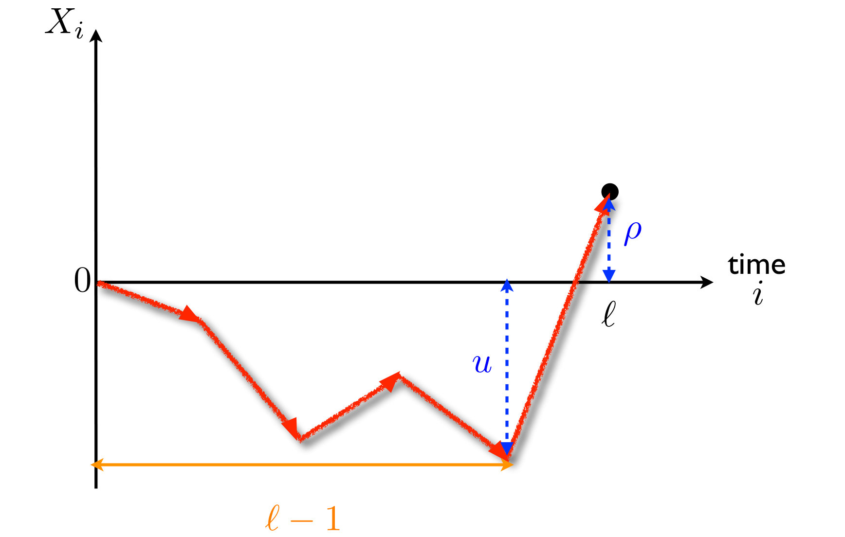 Figure 1
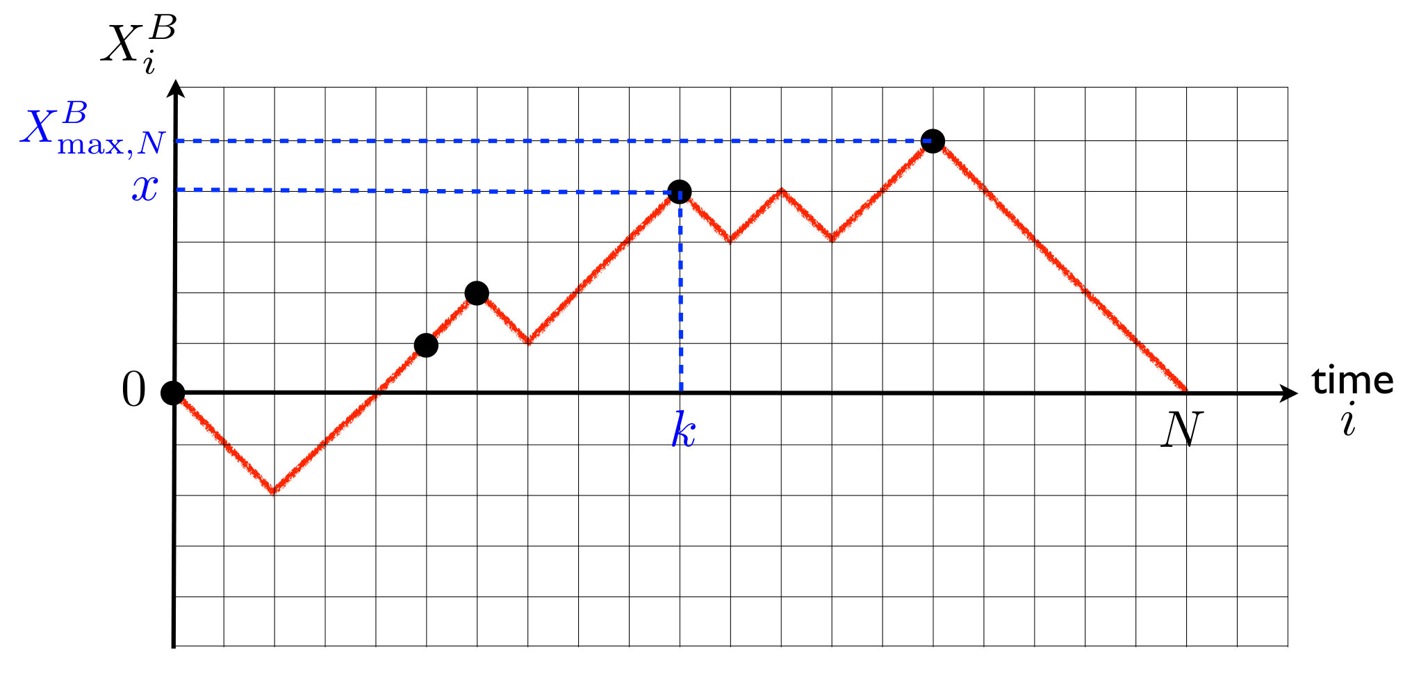 Figure 2
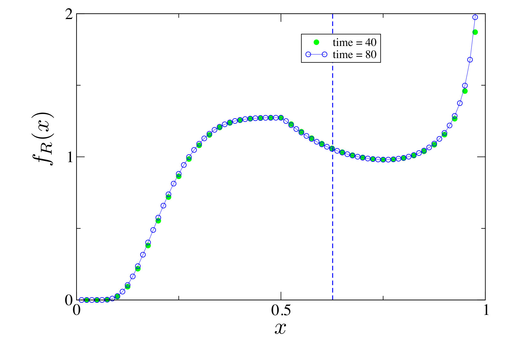 Figure 3
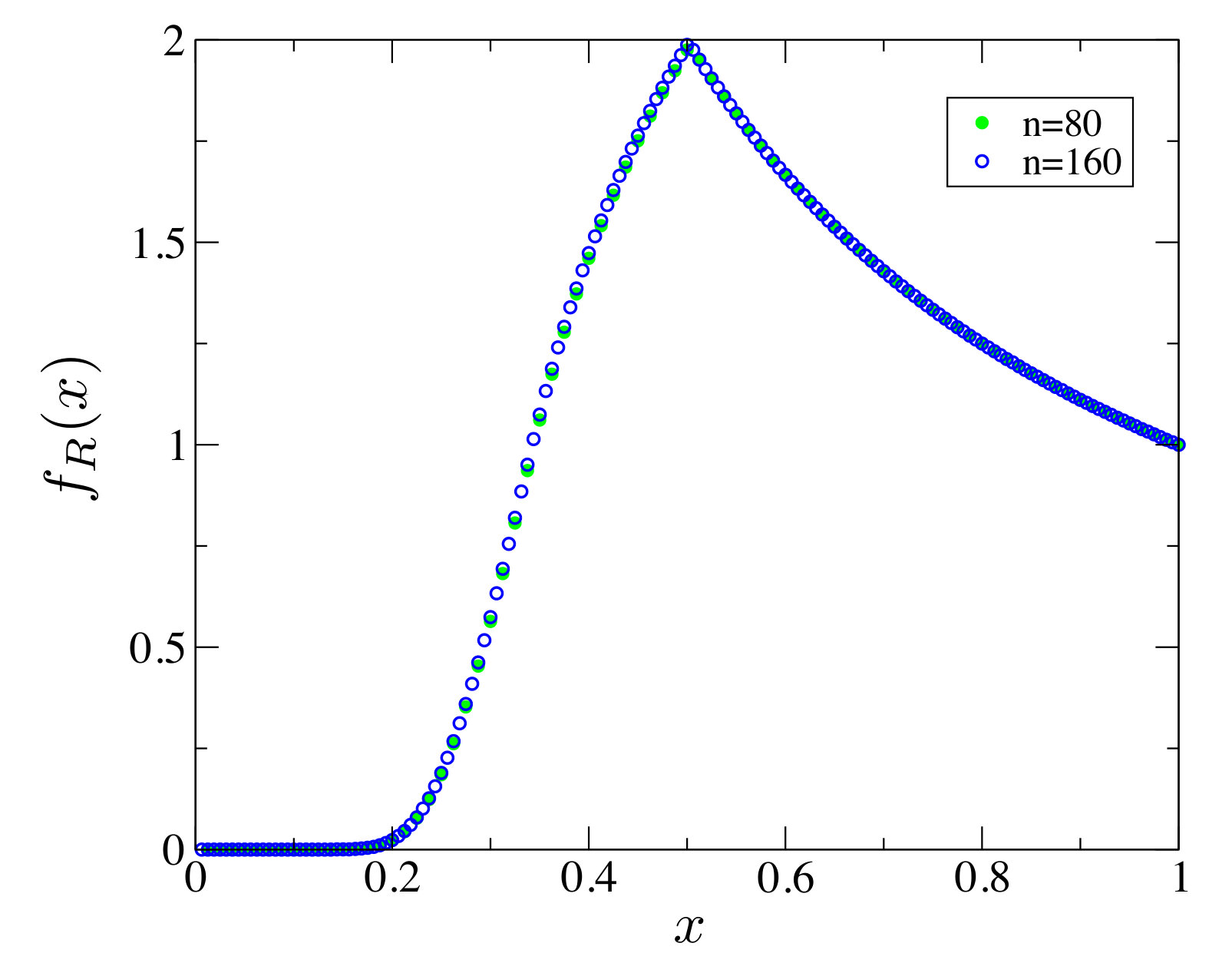 Figure 4
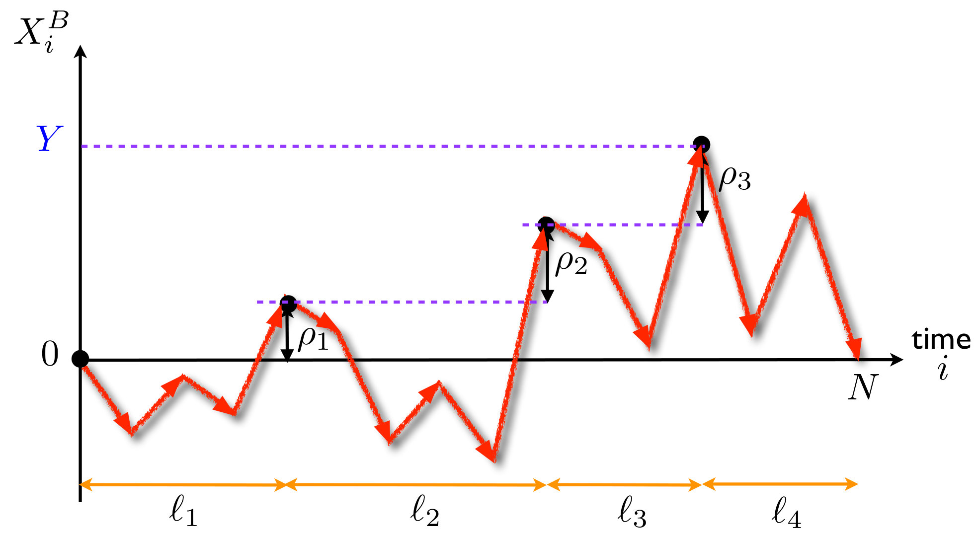 Figure 5
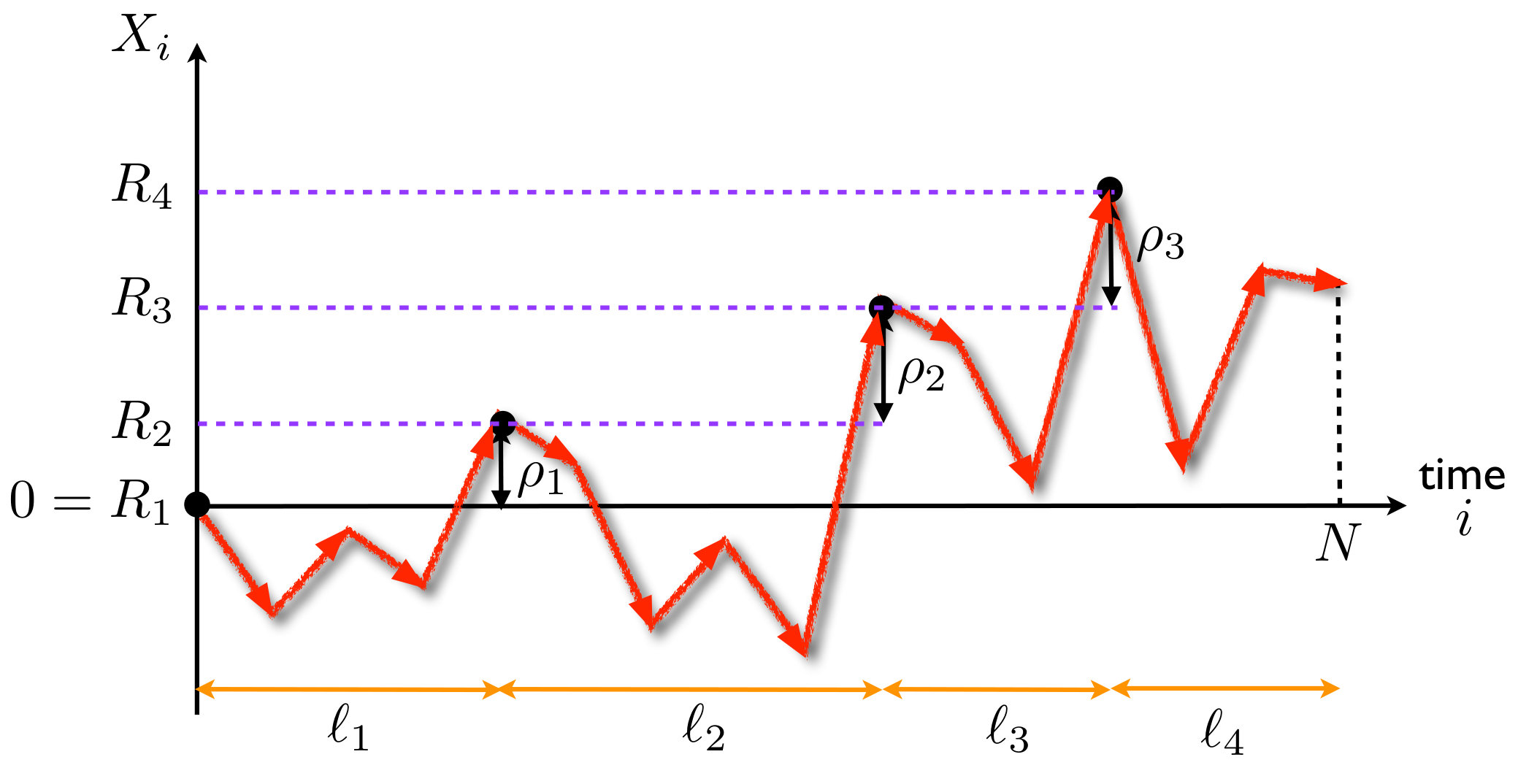 Figure 6
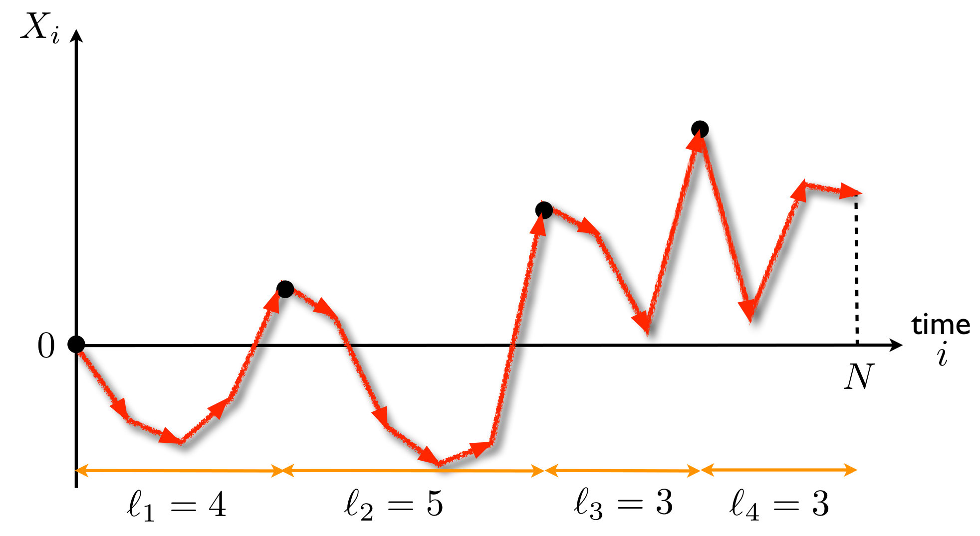 Figure 7
 Figure 8
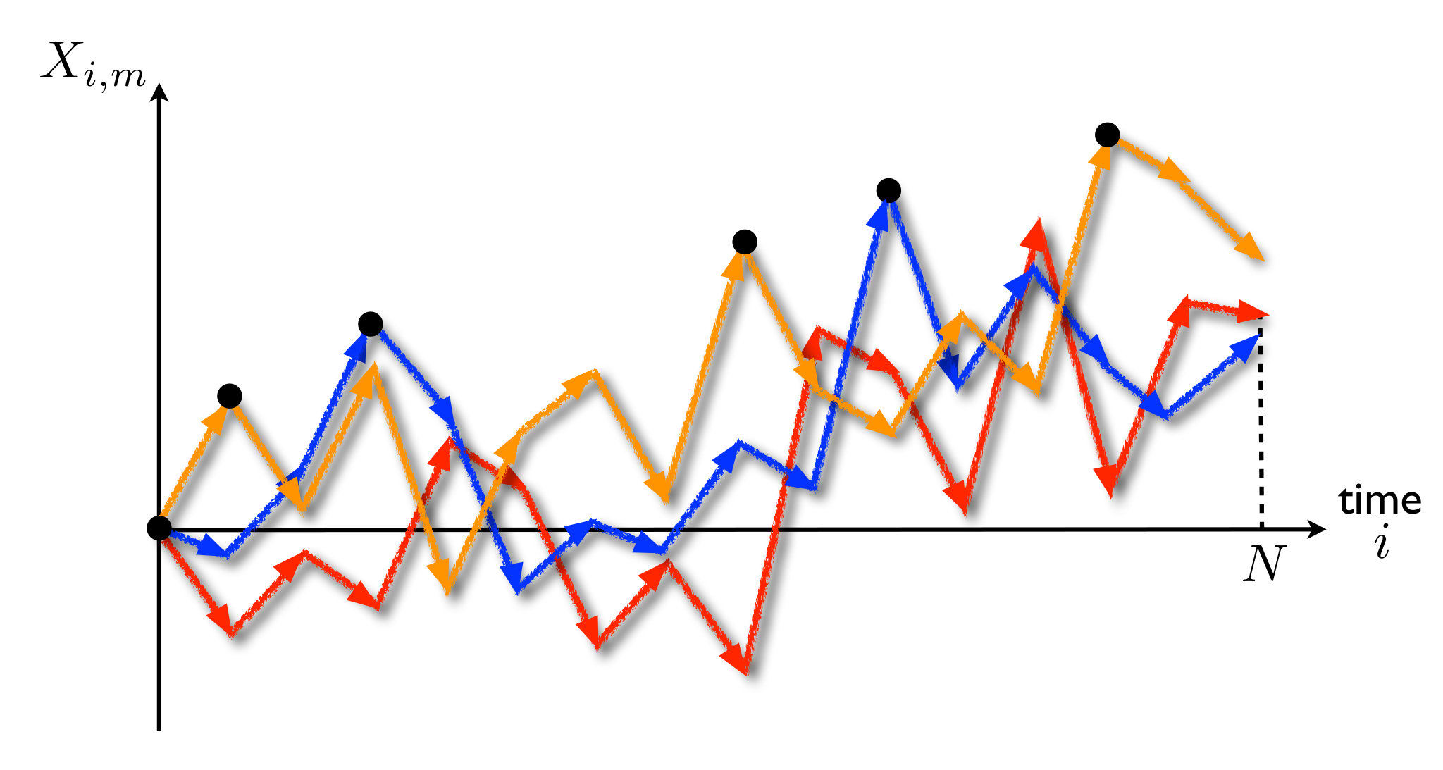 Figure 9
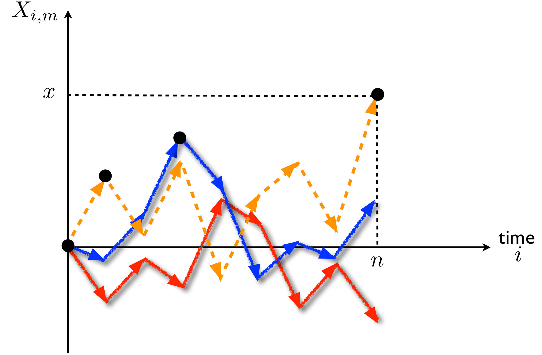 Figure 10
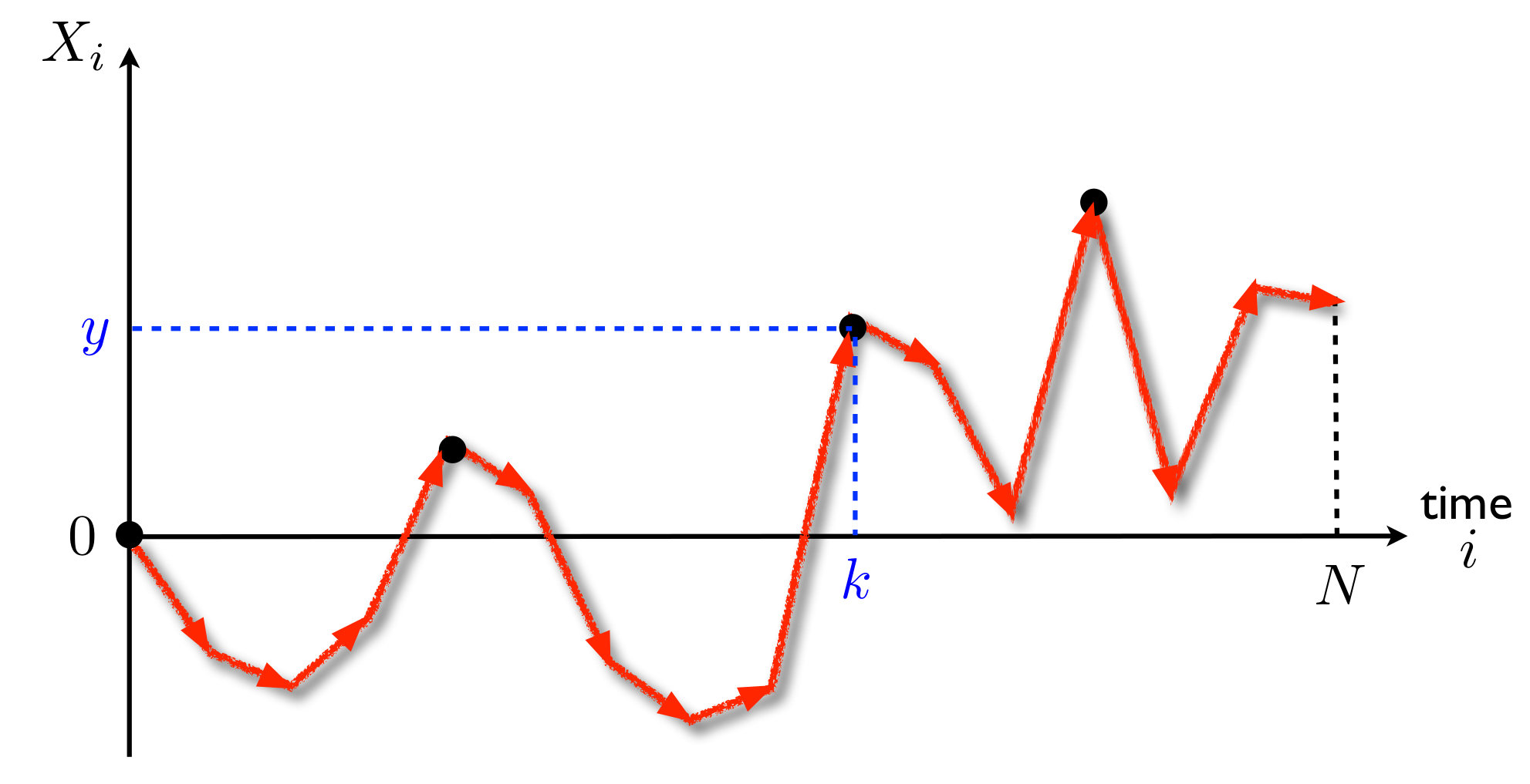 Figure 11
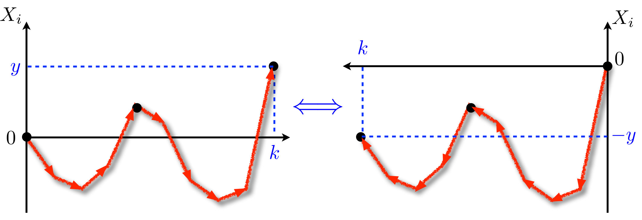 Figure 12
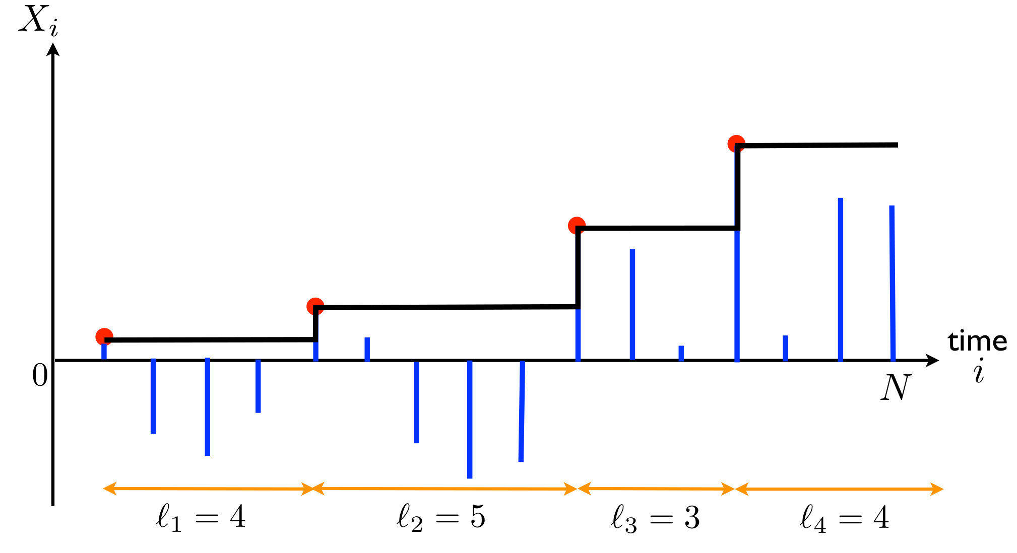 Figure 13
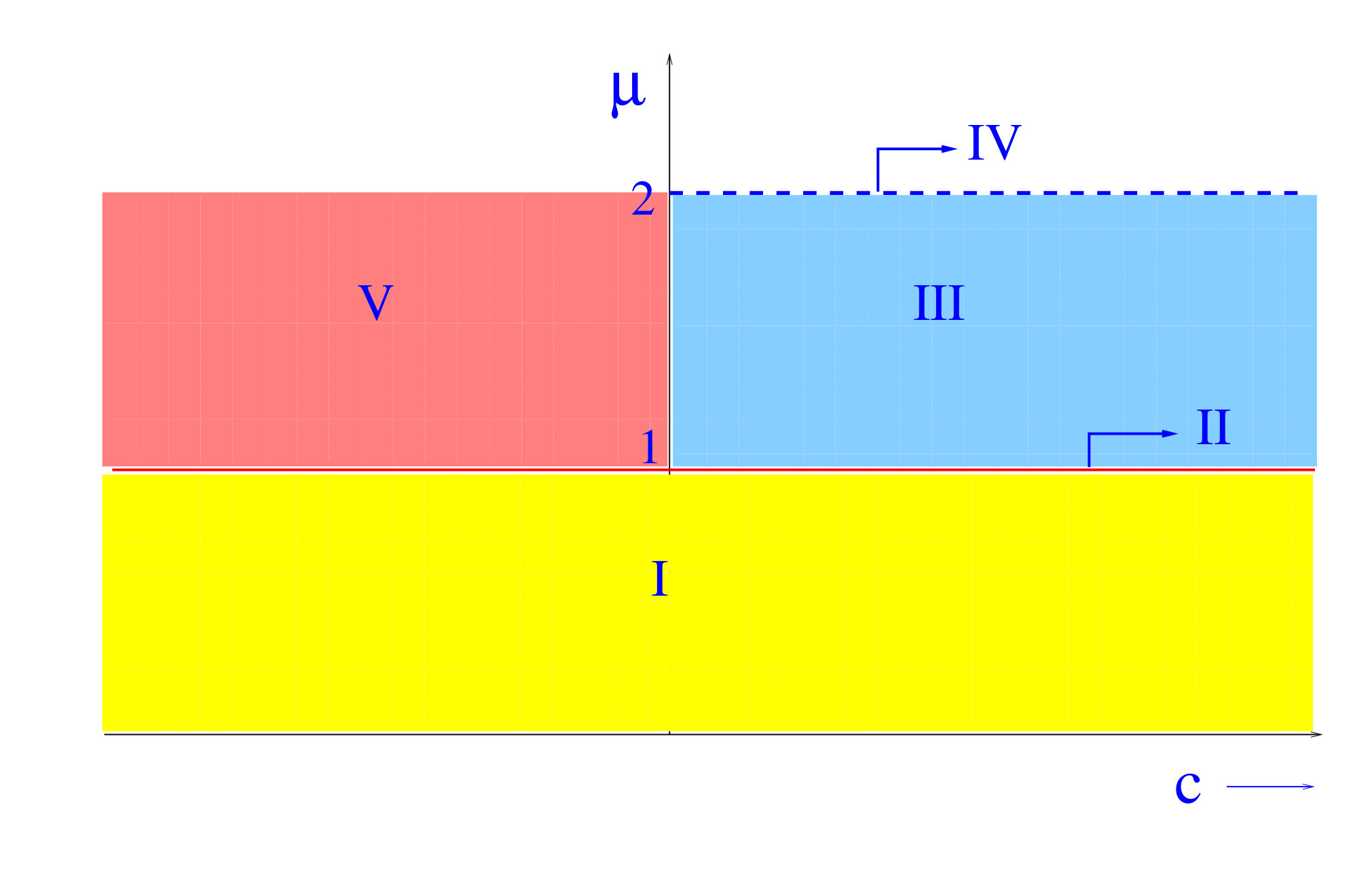 Figure 14
| I | ||
|---|---|---|
| II | ||
| III | ||
| IV | ||
| V |
| I | ||
|---|---|---|
| II | ||
| III | ||
| IV | ||
| V |
Peer Reviews
No public reviews on file for this paper yet. If you reviewed it on a platform where reviews are public (OpenReview, ICLR, NeurIPS, ICML), you can paste yours below so the community can read it here.
Videos
No videos yet. Explain this paper in a talk, walkthrough, or lecture? Add one.
Taxonomy
TopicsCold Atom Physics and Bose-Einstein Condensates · Scientific Research and Discoveries · Statistical Mechanics and Entropy
Record statistics of a strongly correlated time series: random walks and Lévy flights
Claude Godrèche
Institut de Physique Théorique, Université Paris-Saclay, CEA and CNRS, 91191 Gif-sur-Yvette, France
Satya N. Majumdar
LPTMS, CNRS, Univ. Paris-Sud, Université Paris-Saclay, 91405 Orsay, France
Grégory Schehr
LPTMS, CNRS, Univ. Paris-Sud, Université Paris-Saclay, 91405 Orsay, France
Abstract
We review recent advances on the record statistics of strongly correlated time series, whose entries denote the positions of a random walk or a Lévy flight on a line. After a brief survey of the theory of records for independent and identically distributed random variables, we focus on random walks. During the last few years, it was indeed realized that random walks are a very useful “laboratory” to test the effects of correlations on the record statistics. We start with the simple one-dimensional random walk with symmetric jumps (both continuous and discrete) and discuss in detail the statistics of the number of records, as well as of the ages of the records, i.e., the lapses of time between two successive record breaking events. Then we review the results that were obtained for a wide variety of random walk models, including random walks with a linear drift, continuous time random walks, constrained random walks (like the random walk bridge) and the case of multiple independent random walkers. Finally, we discuss further observables related to records, like the record increments, as well as some questions raised by physical applications of record statistics, like the effects of measurement error and noise.
1 Introduction
The statistics of extreme and rare events have recently generated a lot of interest in various areas of science. In particular, the study of the statistics of records in a discrete time series, initiated in the early fifties [1], has become fundamental and important in a wide variety of systems, including climate studies [2, 3, 4, 5, 6, 7, 8, 9], finance and economics [10, 11, 12], hydrology [13], sports [14, 15], in detecting heavy tails in statistical distributions [16], and others [17, 18].
Consider any generic time series of entries where may represent the daily temperature in a given place, the price of a stock or the yearly average water level in a river. A record happens at step if the -th entry exceeds all previous entries. Questions related to records are obviously intimately connected to extreme value statistics [19, 20]. For instance the actual record value at step is just the maximal value of the entries after steps, which is a key observable in extreme value statistics. On the other hand, record statistics has deep connections with first-passage problems [21, 22, 23]. For instance, the record rate, i.e., the probability that a record is broken at step , is related to the survival probability, i.e., the probability that the time series remains below a certain level up to step , which is a key quantity in first-passage problems.
However, despite its connections with extreme value statistics and first-passage problems, the statistics of records of a time series raises specific new questions which require new tools and techniques. In this paper, we focus on a class of observables associated to the record statistics. This includes, for instance, the number of records in a given sequence of size as well as the ages of the records. The age of a record is defined as the time up to which the record survives, i.e., before it gets broken by the next record. We will also study the record values as well as the increments of the record values. The statistics of these observables can not be understood from extreme value statistics or first-passage problems solely and they require new techniques that will be discussed in this review.
Remarkably, the study of records have found a renewed interest and applications in diverse complex physical systems such as the evolution of the thermo-remanent magnetisation in spin-glasses [24, 25], evolution of the vortex density with increasing magnetic field in type-II disordered superconductors [24, 26], avalanches of elastic lines in a disordered medium [27, 28, 29, 30], the evolution of fitness in biological populations [31, 32, 33], jamming in colloids [34], in the study of failure events in porous materials [35], in models of growing networks [36], and in quantum chaos [37, 38] amongst others. The common feature in all these systems is a staircase type temporal evolution of physical observables (see figure 1). For instance, when a domain wall in a disordered ferromagnet is driven by an increasing external magnetic field, its center of mass remains immobile (pinned by disorder) for a while and then, as the field increases further, an extended part of the wall gets depinned, giving rise to an avalanche and, consequently, the center of mass jumps over a certain distance [27, 28, 29, 30]. The position of the center of mass as a function of time (or increasing drive), displays a staircase structure as in figure 1. Some useful insights on such a staircase evolution in these various systems can be gained by studying the dynamics of records in a time series [25, 28, 26], where the record value remains fixed for a while until it gets broken by the next record and jumps by a certain increment (see figure 1). For instance, in the case where the positions are the positions of a random walker after steps, this “record process” is at the heart of the so called ABBM model [29, 30] which has been extensively used to model the so-called Barkhausen noise in disordered ferromagnets [39].
The record statistics for independent and identically distributed (i.i.d.) random variables have been extensively studied in the past, both in the mathematics [40, 41, 42] and also more recently in the physics literature (for a recent review on the i.i.d. case see [18]). Many aspects of these studies are now theoretically well understood and, here, we will briefly recall the main useful results, with a special emphasis on the statistics of the ages, which is somehow less well known. Another class of time series for which record statistics has been studied recently corresponds to independent but non identically distributed random variables. This is quite relevant in sports, where with time the average performance of a sportsman/woman typically increases with time due either to increased nutrition or technologically advanced sports equipments used for the preparation. Similarly in the context of climate studied, there can be a typical linear trend in time of the average temperature. Various interesting results have been derived for this independent but non identically distributed time series [43, 44, 45]. As these results have already been reviewed in ref [18], we will not repeat them here.
In many realistic time series, the entries are however correlated. So, the question naturally arises: what can we say about the record statistics for correlated sequences? For a weakly correlated time series, i.e., with a finite correlation time, one would expect the record statistics for a large sequence to be asymptotically similar to the uncorrelated case. This, however, is no longer true when the entries are strongly correlated. It turns out that in this strongly correlated case, the study of record statistics is technically challenging. The difficulty of the task can be estimated by considering the aforementioned connections with extreme value statistics and first-passage problems, which are notoriously hard to solve for strongly correlated time series. As a consequence, there exist very few results in the literature and in fact all the classical textbooks on records [40, 41, 42] deal essentially, if not exclusively, with the case of i.i.d. random variables.
One of the simplest and most natural strongly correlated time series is the random walk sequence on a line, where the entry corresponds to the position of a random walker at discrete time step , starting from the origin , and undergoing random jumps at each time step. Despite the striking importance and abundance of random walks in various areas of research, the record statistics of such a single, discrete-time random walk with a symmetric jump distribution on a line was not computed and understood until only a few years ago [46]. Indeed, while the positions of a random walker are strongly correlated, the random walk itself is a Markov process. Thanks to this key Markov property, it was recently realized that the random walk and its variants is an ideal laboratory to test analytically the effects of strong correlations on the record statistics of time series.
Indeed, recently, there have been much progress in understanding the record statistics for such a random walk sequence, both with and without drift and also for the case of multiple random walkers, and many interesting analytical results were derived – some of them rather surprisingly universal. This random walk sequence is thus useful as it provides an exactly solvable example for the record statistics of strongly correlated time series. These results for random walks have been briefly reviewed in refs [18, 47, 48]. Since then, however, the subject has rapidly evolved and a detailed account of these recent progresses is still lacking. The purpose of this review is to provide an updated survey of the known results both for i.i.d. and for strongly correlated time series, like random walks and Lévy flights.
The review is organised as follows. We start, in section 2, by a brief survey of the theory of records for i.i.d. random variables. In section 3, we develop the basic theory of record statistics for random walks, which is the cornerstone of this review. These results are based on a general renewal structure which is then exploited to obtain detailed information about the statistics of both the number and ages of the records for several models of random walks, including symmetric random walks – with both continuous and discrete jumps –, random walks with a linear drift and continuous time random walks. In section 4, we focus on the record statistics of constrained random walks, with a special focus on the (symmetric) random walk bridge – i.e., a random walk conditioned to start and end at the origin after steps. In section 5, we discuss the record statistics for independent random walkers and in section 6, we present several generalisations of these results, emphasizing in particular the similarities between the ages of records and the size of excursions between consecutive zeros in the lattice random walk and Brownian motion and more generally in renewal processes. Finally, in section 7, we present some related issues that have been recently discussed in the literature – like the effects of measurement error and noise – before we conclude in section 8.
2 Record statistics for i.i.d. random variables
We begin by reviewing the main results for the record statistics of i.i.d. random variables. We consider a collection of random variables which are drawn from a continuous probability density function () . These random variables being i.i.d., their joint simply factorizes as
[TABLE]
By definition, is an upper record if and only if it is larger than all previous entries,
[TABLE]
For instance in figure 1, is, by definition, a record, then is a record, on so on (see the caption of the figure for details). One can similarly define a lower record which is such that . For now, we will mainly focus on upper records, which we will simply call “records”.
Let be the number of records among these random variables. We first discuss a straightforward method, based on indicator variables, to investigate the statistics of . Then we discuss more complicated joint probability distributions of the number and the ages of the records. This second method is not only useful to investigate the age of the longest and shortest record but can be generalised, with some appropriate modifications, to the study of the records of random walks (see section 3), constrained random walks (see section 4) as well as multiple random walker systems (see section 5).
2.1 Distribution of the number of records
To study the distribution of the number of records it is useful to introduce indicator variables which take the value [math] or :
[TABLE]
For i.i.d. random variables, these indicator functions are independent [see (8) below]. We define
[TABLE]
where the average is taken over the different realizations of the random variables . Thus is the probability that is a record, i.e., that the event in (2) happens. In other words, represents the rate at which a record is broken at “time” , or equivalently the probability of record breaking at time for the sequence . For i.i.d. random variables this probability can be easily computed from the joint distribution in (1) and this yields
[TABLE]
where we have used the change of variable . Interestingly, this result (5) is universal, i.e., it is independent of the parent distribution . This can be easily understood since the probability that is the maximum among is indeed equal to as the maximal value can be realized with equal probability by any of these i.i.d. random variables. From the record rate in (5), we get the mean number of records as
[TABLE]
where denotes the -th harmonic number. For large , it behaves as
[TABLE]
where is the Euler constant. By a similar calculation, one can compute the variance of the number of records, . This computation involves the two-point correlations . From the joint distribution (1) it is easy to show that and are linearly independent for [48]. Indeed, by a simple generalisation of the reasoning made above for (5), one has
[TABLE]
while . Hence, using (8), one obtains
[TABLE]
Similarly, one can compute the generating function of the probability distribution of the number of records using (for )
[TABLE]
where is the Gamma function. One also recognizes that the ratio of Gamma functions appearing in (10) is the of the unsigned Stirling numbers of the first kind [49], i.e.,
[TABLE]
where the unsigned Stirling numbers enumerate the number of permutations of elements with exactly disjoint cycles. Hence one has
[TABLE]
which thus shows that the number of records of i.i.d. random variables is distributed like the number of cycles in random permutations of objects with uniform measure. Finally, using the asymptotic behaviour of Stirling numbers, one can show that the distribution of approaches, when , a Gaussian distribution
[TABLE]
Here we have discussed the case where the random variables are continuous random variables. We refer the reader to ref [50] for a discussion of the effects of discreteness, in particular when continuous random variables are subsequently discretized by rounding to integer multiples of a discretization scale (see also section 7 for related issues).
2.2 Joint distribution of the ages of records and of their number
Apart from the number of records, other important observables are the ages of the records, which we now focus on. For a realization of the sequence of random variables with records, we denote by the time intervals between successive records as depicted in figure 1. Thus is the age of the -th record, i.e., it denotes the time up to which the -th record survives (in the mathematical literature the ages are called “inter-record times” [41, 51]). Note that the last record, the -th record in this sequence, is still a record at “time” . Its age is defined as its lifetime shifted by one unit, where is the time of occurrence of this last record (see figure 1). This definition simplifies the computations that follows.
We first compute the joint probability distribution of the ages and the number of records, given the length of the sequence. This distribution can be computed from the joint distribution of the in (1) as
[TABLE]
where the Kronecker delta, if and 0 otherwise, ensures that the size of the sample is . If one performs the change of variables , the distribution in (2.2) can be written as
[TABLE]
This multiple integral in (15) can be performed straightforwardly to obtain
[TABLE]
It is important to stress that this joint distribution is completely universal, i.e., independent of the parent distribution . This means that any observables depending only on the ages of the records is totally universal. Quite interestingly, although the variables are independent, we see on (16) that the ages are correlated, which yields a non trivial statistics of the ages in this i.i.d. case. In the next section we discuss the marginal distribution of the age of the -th record as well as the statistics of the longest or shortest records and refer the reader to ref [52] – chapter 1 – for further details and references on the ages of records for i.i.d. random variables in the mathematical literature.
We conclude this section by a remark on the record times, which are the times at which the records occur,
[TABLE]
with . Elements of the study of these record times can be found in [36]. In particular, in the continuum limit of large times, these record times, now real variables denoted by , are generated recursively. The successive ratios
[TABLE]
are i.i.d. random variables uniform on . This property is instrumental in the derivation of the asymptotic distribution of the duration of the longest lasting record [36] [see (29-30) in section 2.4 below].
2.3 Marginal probability distribution of the age of the -th record
The marginal probability distribution of can be obtained by summing the full joint distribution in (16) over all the ages with and then summing over the number of records:
[TABLE]
The full distribution , given in (16), is obviously not invariant under the permutation of the ages and therefore depends explicitly on . Its with respect to can be computed exactly – using the integral representation of the full joint distribution (15) – with the result [53]
[TABLE]
We see that the right hand side of (20) behaves like when , from which we conclude that tends to a stationary distribution as , which is given by [51, 54]
[TABLE]
where the second line is obtained by performing the change of variable in the integral in (2.3) and using the binomial formula to expand in order to perform the integral over . The probability is a monotonically decreasing function, starting from . For large , its asymptotic behaviour is more conveniently obtained from the integral representation (2.3) which can be analysed in the large limit by performing the change of variable which yields
[TABLE]
This indicates that the first moment of is diverging when . In fact, one can show from (20) that
[TABLE]
Interestingly, by using the Stirling formula , one sees that the average , as a function of , admits a maximum for , for which (up to possible logarithmic corrections). Hence, coincides with the typical number of records , see (7). This indicates that the longest lasting record is rather likely to be the last one, which happens with a rather high probability [see (28) and (34) below], or close to it [53]. The statistical properties of the longest lasting record will be discussed in the next section.
2.4 Distribution of the age of the longest lasting record
We have seen in the previous section that the mean age of the -th record, , depends rather strongly on , see (23). It behaves typically as as a function of and reaches its maximum for where it is of order . In this section, we characterize this extreme behaviour and focus on the age of the longest record, denoted by , which is defined as
[TABLE]
Its cumulative distribution , for , is obtained from the full joint distribution in (16) by summing over and with the constraint that , , . It reads, for ,
[TABLE]
while . The of with respect to is conveniently written using the integral representation of the distribution in (15). After some manipulations, it can be written as [48]
[TABLE]
From the of the full distribution of (26) one obtains the of the average value as
[TABLE]
By analysing this expression (27) in the limit , where the discrete sums can be replaced by integrals (setting ) one obtains the large behaviour of as
[TABLE]
where . In (28), is known as the Golomb-Dickman or Goncharov constant [55]. This constant also describes the linear growth of the longest cycle of a random permutation [55]. It also appeared in a model of growing network [36] and in a one-dimensional ballistic aggregation model [56]. The complete asymptotic expansion of , beyond the leading order, was established in ref [57].
A complementary approach to the statistics of can be found, e.g., in refs [36, 58]. In particular, in the regime of long times the scaled random variable has a limiting density denoted by ,
[TABLE]
To compute this limiting distribution , it is convenient to study the inverse variable , which has a limiting density . It turns out that the Laplace transform of the inverse variable has an explicit expression
[TABLE]
where we recall that . Note that from (30) one can straightforwardly compute the average as
[TABLE]
which, after a simple integration by parts, yields back the Golomb-Dickman constant in (28), i.e., . Furthermore, from (30), and using , one can show that the function is a piecewise continuous function on the interval , continuous on each interval of the form , , , and exhibiting singularities at the points , with . It has a maximum at and its asymptotic leading behaviours are given by [36]
[TABLE]
We refer the reader to ref [36] for further details on this limiting distribution. Figure 2 depicts obtained from the analytical expression of the generating function of given by (26) for (green full circles) and (blue empty circles). The good collapse of the data confirms the scaling form (29).
Another, related, quantity of interest is the probability that the longest lasting record is the last one, or probability of record breaking for the sequence of ages, namely
[TABLE]
This sequence converges, at large , to the Golomb-Dickman constant [36],
[TABLE]
which means that, for a very long sequence, the fraction of records with longest duration is equal to .
2.5 Distribution of the age of the shortest record
We now focus on the age of the shortest record, denoted by , which is defined as
[TABLE]
We define , , and . Using the same reasoning as above for we find the of with respect to as
[TABLE]
The of the average value can be obtained from (36) which yields the asymptotic result for large [59]
[TABLE]
with the numerical value , where is the Euler constant.
On the other hand, when , one can easily show that converges to a stationary cumulative distribution function, from which one obtains the limiting distribution
[TABLE]
while . The limiting distribution is a monotonously decreasing function of and its asymptotic behaviours are given by
[TABLE]
Remembering that this asymptotic behaviour for large , , is valid for , this yields the large estimate for as given in (37). In figure 3 we show a plot of this limiting distribution , where we see in particular that the asymptotic large behaviour (39) gives a quite accurate description of the exact distribution already for .
3 Record statistics for correlated sequences: Random Walk model
We have seen in the previous section that for an uncorrelated time series of length , the statistics of the number of records , as well as the statistics of the ages of records can be computed analytically. In many realistic time series, the entries are however correlated. So, the question naturally arises: what can we say about the record statistics for correlated sequences? We review below the recent results that have been obtained for the random walk sequence.
We start with the simple case of a discrete-time random walk on a line. This will include both short-ranged random walks as well as long-ranged Lévy walks as explained below. In addition, it may include random walks in the presence of a constant drift. The walker starts at the origin and its position evolves in discrete-time via the Markov rule
[TABLE]
where represents the random jump length at step . These noise variables are i.i.d. random variables, each drawn from the jump distribution . The jump distribution may be symmetric (no drift) or asymmetric (e.g., in the presence of a constant drift).
Few examples of symmetric jump distributions are:
- (i)
(exponential),
- (ii)
(Gaussian),
- (iii)
(uniform in ),
- (iv)
for large with (Lévy flights),
- (v)
(lattice random walk).
In the first four examples, the jump distribution is continuous. In the last example, the jump distribution is not continuous, and the walker is restricted to move on a one-dimensional lattice with unit lattice spacing. For the first three examples, the variance of the step length is finite, while in the Lévy case, is infinite.
Note that even though the noise variables are uncorrelated, the positions are strongly correlated. We consider such a sequence of entries with records. For an illustration, see figure 4. Our first goal is to compute the distribution of the number of records . We will also be interested in the statistics of the ages of the records. The random variable denotes the age of the -th record, i.e., the length of time between the -th record and the -th record (see figure 4). The ages are thus defined as in the i.i.d. case (see figure 1), except for the last one. In both cases one sets . However the origins of time are different in the two cases, namely for i.i.d. variables the first record starts at time 1, while for the random walk it starts at time zero. Hence there is a shift of one unit between the two ages . In figure 1 one has , while in figure 4 one has .
Hence our main observables are the number of records , and the ages of the records. Following the i.i.d. case investigated in the previous section (see (3) and below), we can still write , where is a binary variable: if a record occurs at step and otherwise. However, unlike in the i.i.d. case, the variables are now correlated in the random walk case. Hence, it is hard to compute directly the distribution of . So, how does one proceed to compute in this case?
We will see below that one can make progress in calculating by using the renewal property of the random walk. Indeed this approach was used in ref [46] to compute exactly for symmetric jump distributions. But the renewal property is more general, and can be used even for random walk sequence with a drift [60, 61], as we will see below. For introductions to renewal processes, see, e.g., [62, 63, 64].
3.1 The general renewal property
Following ref [46], we note that instead of trying to compute directly, it is convenient to first consider a bigger collection of random variables in a given sequence, namely the number of records as well as the collection of their ages denoted by the vector . The joint distribution of these random variables will be denoted by as in the i.i.d. case. The main point is that this apparently more complicated joint distribution actually has a rather simple structure, due to the renewal property (as explained below). Consequently, by integrating out the age variables from the joint distribution, one can exactly obtain the marginal distribution of the record number only.
Our goal now is to first compute the joint distribution for the generic random walk sequence. For this, we will need two crucial quantities as building blocks [46].
- •
The first quantity is the so called persistence or survival probability . It is the probability that a random walk, starting at the initial position , stays below up to step
[TABLE]
with by definition. In going from the first to the second line in (41), we have used the translation invariance of the process with respect to the starting point. Evidently, does not depend on and we can set . For later purposes, let us also define its generating function
[TABLE]
- •
The second ingredient is the related first-passage probability (starting at ) and defined as
[TABLE]
It is clear that is simply related to via
[TABLE]
Consequently, the generating function of is simply related to that of as
[TABLE]
We will see later that both probabilities and for a random walk can be computed exactly. But for now, we can proceed even without the explicit knowledge of the two. In fact, the discussion below will hold for any arbitrary renewal process, not necessarily restricted to the random walk sequence.
Armed with these two probabilities and , and using the fact that the successive intervals between records are statistically independent due to the Markov nature of the process (also called the renewal property), it follows immediately that (see figure 4)
[TABLE]
where the Kronecker delta enforces the global constraint that the sum of the time intervals equals . The fact that the last record, i.e., the -th one, is still surviving as a record at step indicates that the distribution of the last interval is different from the preceding ones. It is easy to check that is normalised to unity when summed over and .
The record number distribution is just the marginal of the joint distribution when one sums over the interval lengths. Due to the global constraint, this sum is most easily carried out by considering the generating function with respect to . Multiplying (46) by and summing over and , one arrives at the fundamental relation
[TABLE]
where we used (45). Thus the knowledge of enables one to determine the distribution and all its moments. For instance, multiplying (47) by and summing over all , one obtains the exact generating function of the average number of records in steps
[TABLE]
Similarly, the higher moments can also be computed in principle, once one knows .
Let us emphasize again that the result (47), and consequently (48) are rather general, and hold for any renewal process. So, we only need to know . This, however, can be computed explicitly for any random walk process on a line using an elegant theorem due to Sparre Andersen [65]. According to this theorem, the generating function satisfies a nontrivial combinatorial identity [62, 65]
[TABLE]
where . Note that involves a non-local property of the trajectory from the [math]-th to the -th step, namely it is the probability that stays negative up to step , starting at the origin. In contrast, is a local quantity: it is the probability that exactly at step , the walker is on the negative side of the origin.
In the next subsections, we will consider several cases where , or equivalently can be computed explicitly using this theorem, leading to exact results for .
3.2 Statistics of the record number
In this subsection, we will apply the general renewal theory developed above to compute explicitly the distribution of the record number for a random walk sequence for a variety of jump distributions, with and without drift.
3.2.1 Symmetric and continuous jump distribution.
For symmetric and continuous jump distributions (see examples (i)-(iv) discussed in the introduction of section 3), clearly for all (by symmetry). Consequently, (49) gives
[TABLE]
a completely universal result, i.e., independent of the jump distribution , as long as it is symmetric and continuous. Expanding in , it gives the universal result
[TABLE]
Let us remark that this result for is universal for all . Consequently, from (47), the record number distribution also becomes universal for all [46]. For instance, substituting (50) in (47) and inverting with respect to gives the exact distribution, universal for all (equations (52)-(56) were first derived in [46])
[TABLE]
From this exact result in (52) all moments of can be computed as well. For example, the average number of records is given by
[TABLE]
In particular, for large , the mean number of records grows as
[TABLE]
much faster than the logarithmic growth for i.i.d. sequences discussed in the previous section [see (7)]. It is easy to show from the exact distribution that the variance grows linearly for large
[TABLE]
Thus, both the mean and the standard deviation grow as for large , indicating that the fluctuations are large. This is also vindicated by the scaling analysis of the distribution in (52) in the scaling limit, by setting and taking the limit. In this scaling limit, one obtains
[TABLE]
where is the Heaviside step function (i.e., if and if ). Indeed, this scaling behaviour of for the random walk case is markedly different from the i.i.d. case discussed before in (13), where approaches a Gaussian distribution , with mean and standard deviation .
We conclude this subsection by noting that the mean record number can easily be computed following the rationale presented in the i.i.d. case (3)–(6), and using the Sparre Andersen theorem.
Indeed, as in the i.i.d. case, the mean record number can be computed as
[TABLE]
where is the record rate at step , i.e., the probability that a record occurs at step , as in figure 5. To compute the probability of such an event, we isolate the first steps of the trajectories (as does not depend on the positions of the random walker with ), as in figure 6, and we denote by the actual value of the record at step . Next, we choose as a new origin of the random walk the last point, with coordinates , and we change the direction of the time axis (see figure 6). In this new frame, we see that the event depicted in figure 6 contributes to the probability that the random walk starts from the origin and arrives at after time steps, staying negative in between.
By integrating over the final position , one obtains that the rate is precisely identical to the survival probability as defined in (41). Thus, from (57), and using the Sparre Andersen theorem (51), one obtains
[TABLE]
recovering the result obtained in (53) in a different manner. We will see that this way of computing the average number of records (57) can be generalised to the case of a random walk bridge (see section 4) and multiple random walks (see section 5).
3.2.2 Symmetric random walk on a lattice.
This case corresponds to the random walk sequence with a non-continuous jump distribution, . Since the walker starts at , the walk stays on the one-dimensional lattice with unit lattice spacing. For such a sequence , there are evidently a lot of degeneracies. We will count an entry as a record if it is strictly bigger than all previous entries, i.e., if . The general renewal result for the record number distribution in (47) still holds for this case, but is no longer given by the simple form that is only valid for symmetric and continuous jump distributions. However for the lattice walk can be computed explicitly either by standard generating function techniques [62] or via the Sparre Andersen theorem in (49). We illustrate below both methods for completeness.
To compute for a lattice random walk starting at the origin, it is convenient first to consider , which denotes the probability that starting at , the walker does not go to the negative side (but can come back to the origin) up to step . Clearly, . It is easy to see that satisfies a backward recurrence equation [23, 62], for
[TABLE]
with the boundary condition and non-divergent for all , and the initial condition for all . The generating function then satisfies the recursion relation
[TABLE]
This linear recursion relation can be trivially solved for the appropriate boundary conditions given above, yielding, for all
[TABLE]
In particular, we get
[TABLE]
In particular, when , , yielding
[TABLE]
which differs by a factor from the result in (51) obtained for continuous jump distributions.
It is amusing to see how the same result in (62) can also be derived from the Sparre Andersen theorem in (49). For this, we need to compute . Note that for lattice walks, . Using the symmetry and the fact that the total probability adds up to unity, we have . Hence, we get
[TABLE]
But the of the return probability to the origin can be trivially computed [62]
[TABLE]
Using this result on the right hand side of (49) and a few steps of straightforward algebra gives us the desired result in (62).
Substituting the exact from (62) in (47) then gives us the exact for lattice walks. One can also compute all the moments of exactly. For instance, substituting in (48), we get [46]
[TABLE]
which, when inverted, gives [46]
[TABLE]
where is the standard hypergeometric function. For , , , , , one gets respectively. In particular, for large , one has
[TABLE]
which is smaller by a factor than the expression for the mean number of records in the continuous case given in (54).
The full distribution of the record number can also be obtained using the general formula in (47) and the appropriate result for the survival probability for the discrete random walk in (62). However, this distribution can be obtained more directly for the lattice random walk by noticing the connection between the number of records and the maximal displacement of the random walk up to step , i.e., . This relation reads [66]
[TABLE]
To derive this relation (69) it is useful to consider the time evolution of the two processes and as increases. At the next time step , if a new site on the positive axis is visited for the first time, the process increases by , otherwise its value remains unchanged. On the other hand, when this event happens, then the record number is also increased by one, and otherwise it remains unchanged. Therefore we see that the two processes are locked with each other at all steps. Since, by convention, the first position is a record implying that initially , while , one obtains immediately the relation in (69). From this relation it is possible to obtain the statistics of from the one of , which can be computed easily, e.g., using the method of images. This yields [66], for
[TABLE]
where denotes the smallest integer not less than . One can check that this exact formula for the distribution (70) yields back the result in (67) for the first moment. In addition, in the large limit the probability distribution takes the scaling form
[TABLE]
which is similar, up to a factor as already noticed below (67), to the result obtained for continuous jump distributions in (56). This scaling form (71) can be understood by reminding that the lattice random walk properly scaled, with , converges for large to the standard Brownian motion with diffusion coefficient on the unit time interval . Hence one expects from the identity in (69) that converges for large to the maximum of the Brownian motion on the unit time interval, which is indeed given by the half-Gaussian in (71). As we will see later, this identity (69) can be used to compute the record statistics of constrained random walks, like random walk bridges (see section 4) or the one of multiple random walks (see section 5).
3.2.3 Random walk in the presence of a constant drift.
In this subsection we will study the record statistics for a sequence where denotes the position of a one-dimensional random walker at step (discrete time and continuous space), in the presence of a constant drift . The position evolves in time via the Markov rule (starting from )
[TABLE]
where are i.i.d. jump variables as before.
To keep the discussion simple, we will restrict ourselves to the case of a symmetric and continuous jump distribution . We will see later that in the presence of a nonzero drift , the asymptotic tail of the symmetric jump distribution for large plays a rather crucial role. These tails can be nicely characterized in terms of the Fourier transform of the jump distribution. We will focus below on a large class of jump distributions whose Fourier transform has the following small behaviour
[TABLE]
where and represents a typical length scale associated with the jump. The exponent dictates the large tail of . For jump densities with a finite second moment , such as Gaussian, exponential, uniform etc., one evidently has and . In contrast, corresponds to jump densities with fat tails as . A typical example is where corresponds to the Gaussian jump distribution while corresponds to Lévy flights (for reviews on these jump processes see [67, 68]).
In this subsection, we are interested in computing the statistics of the record number for the sequence in (72), for a nonzero constant drift . In fact, this problem was first studied in ref [60] for the special case of Cauchy jump distribution [which belongs to the family of jump densities in (73)]. By using the renewal approach mentioned above, it was found that the mean number of records in this Cauchy case grows asymptotically for large as [60]
[TABLE]
In addition, the asymptotic record number distribution for large was found [60] to have a scaling distribution, with a nontrivial scaling function which reduces, for , to the half-Gaussian in (56).
For jump densities with a finite second moment and in the presence of a nonzero positive drift , the mean number of records was analysed in ref [11] and was found to grow linearly with for large , , where the prefactor was computed approximately for the Gaussian jump distribution. However, an exact expression of the prefactor for arbitrary jump densities with a finite was still missing. These results for the mean record number were then compared to the stock prices data from the Standard and Poors 500 [11].
Finally, in ref [61], the full distribution of the record number for large was analysed in detail for the whole family of continuous and symmetric jump distributions with Fourier transforms as in (73), for all and all . An extremely rich behaviour for the record statistics was found [61] for varying and (see below). Here we just summarise the main steps behind this analysis and the main results (for details we refer the reader to ref [61]). There are three main steps for the computation of record statistics that are described as follows.
- •
To use the general renewal approach outlined in the previous subsection, which is valid for arbitrary . The only requirement is the knowledge of the persistence probability .
- •
The persistence probability can be estimated from the Sparre Andersen identity in (49), which is also valid for arbitrary . One needs to just evaluate the local quantity . For this one needs to know the probability distribution at step of the walker evolving via (72). In fact, for the asymptotic analysis of record number, it suffices to know the behaviour of for large , which in turn requires the knowledge of for large . This latter quantity has been well studied in the literature and one has a rather complete knowledge of this distribution [67, 68]. Using this, one can estimate and hence via the Sparre Andersen identity. This was carried out in detail in ref [61] for all and all . A summary is provided in the table 1 below.
- •
Once is known for large , one can then use the renewal results in equations (48) and (47) to estimate respectively the mean number of records and the record number distribution , asymptotically for large [61].
As mentioned above, both the persistence and the mean record number (as well as the distribution ) display a rather rich and varied behaviour as functions of and [61]. On the strip (see figure 7), it turns out that there are five distinct regimes: (I) when with arbitrary (II) when and arbitrary (III) when and (IV) when and and (V) when and .
In each of these five regimes the persistence and the mean record number have different asymptotic dependence on the sequence size for large (see table 1). Consequently, also displays different scaling distributions in the five phases. The line (regime II above) is a critical line on which both the persistence and the mean record number exhibits marginal behaviour, in the sense that the exponents characterizing the asymptotic behaviours of these quantities depend continuously on the drift .
Without giving further details, we just summarise in table 1 the asymptotic behaviour of and in these five regimes in the strip in figure 7. Let us make few remarks concerning the asymptotic results presented in table 1. The prefactors for the persistence in the second column of table 1 can be computed exactly [61]. In the marginal case (regime II, i.e., along the line in figure 7), the persistence exponent was first computed in ref [69]. The constant was computed in ref [61]. Finally, the constant prefactors appearing in the asymptotic expressions for in the third column of table 1 are also explicitly computable [61]. Finally, the full scaling forms of the record number distribution for large are also computed explicitly in ref [61] in all the five regimes. Note that the results obtained in the region IV (corresponding to and arbitrary ) were extended in ref [70] to a wider class of random walks with stationary correlated jumps (and no assumption on the symmetry and/or continuity of the jump distributions).
We conclude this section by mentioning that these results for the record statistics of random walk with a drift were used in the context of finance, in [71, 72], to demonstrate that records provide a useful unbiased estimators of the so-called Sharpe ratios – which characterize the signal-to-noise ratio of a financial time series, like the one generated by the time evolution of a price return. We refer the reader to [71, 72] for more detail on this question as well as to [73] for an implementation (an R-package) of this estimator.
3.2.4 Continuous-time random walk.
Another model where the general renewal approach outlined above can be exploited to compute exactly the record number statistics [74] is the so called continuous-time random walk model, introduced by Montroll and Weiss [75]. In the continuous-time random walk model, both space and time are continuous. The walker moves on a continuous line by successive jumps as before, with jump lengths drawn independently from the distribution . However, between two jumps, the walker waits for a random amount of time drawn, independently for each jump instance, from a waiting time distribution . One considers waiting time distributions with a power law tail for large . If , the mean waiting time is finite and in this case the walker essentially behaves like a discrete-time random walk as discussed earlier. However, interesting new behaviour emerges when the mean waiting time is divergent, i.e., in the case when (see the reviews [67] and [68] for detailed discussions). In this case, the Laplace transform of the waiting time distribution behaves as
[TABLE]
where is a microscopic time scale.
To compute the record statistics, one can again use the general renewal approach outlined before, except that now one considers a continuous-time analogue of (46) that reads
[TABLE]
where the subscript stands for the continuous time. Here, denotes the collection of ages of records and is the joint distribution of the ages and the number of records in time . Note that in this expression (76), the variables (as well as ) are continuous and, consequently, the function is a Dirac delta function and no longer a Kronecker delta as for the discrete-time random walk (46).
The function denotes the probability that the walker stays below [math] up to time . Similarly, denotes the first-passage probability density, i.e., denotes the probability that the process, starting at the origin, crosses to the positive side for the first time in the time interval . Taking the Laplace transform of (76) with respect to and integrating over gives
[TABLE]
where . In deriving the last equality in (77) we have used which follows by taking the Laplace transform of the relation . In (77), is just the probability of having records in time . Hence (77) is the exact continuous-time analogue of (47) derived earlier.
To make further progress, we need to determine in terms of the waiting time distribution . This can be easily done as follows. Consider a time interval between two successive zero crossings that contains exactly jump events. For fixed , clearly the number of possible steps is a random variable. Its distribution can be easily computed using the fact that successive waiting time intervals are statistically independent, i.e.,
[TABLE]
Taking Laplace transform with respect to gives
[TABLE]
Using , one observes immediately that
[TABLE]
where is precisely the first-passage probability in discrete step , defined before in (43). Taking Laplace transform of (80) and using (79) then gives
[TABLE]
where is the generating function of the first-passage probability of the discrete-time random walk. For example, for symmetric and continuous jump distribution , we have from (45). Hence, in this case, plugging (81) in (77) gives the following main result [74]
[TABLE]
While the Laplace transform in (82) is not easy to invert for arbitrary , one can make progress in the scaling limit for large , large but keeping the product fixed. In this limit, using the small behaviour of in (75) one obtains a limiting scaling distribution [74]
[TABLE]
where the scaling function is given by
[TABLE]
The function is the standard one-sided Lévy stable density. Note that for , one can show [74] that the result in (83) reduces to the half-Gaussian result in (56), as one would expect.
Thus, to summarise, for the continuous-time random walk with waiting time distribution and jump length distribution , the distribution of the record number in time is independent of the jump distribution (for symmetric and continuous ), but does depend on the waiting time distribution . For power-law waiting time distribution, as with divergent mean, i.e., , has a scaling form as in (83) and the typical number of records grows with time as, for large . In the borderline case , one recovers the discrete-time result discussed earlier.
3.3 Statistics of the ages of records for random walk models
Apart from the number of records, other interesting observables are the ages of the records of a random walk sequence. As defined in the introduction of section 3, the age of the -th record is the number of steps between the -th and ()-th records, i.e., the time up to which the -th record survives (see figure 4). Note that the last record is still a record at step and hence the last age is not on the same footing as the other ones.
Thanks to the (spatial) translational invariance of the random walk (see e.g., (41)), the sets of the ages behave similarly to the intervals between two consecutive zeros of a lattice random walk – in other words to the lengths of the excursions. Hence, as we will see below, the study of the ages of the records for a random walk bears strong similarities with the excursion theory of the lattice random walk and Brownian motion.
As we discuss it in this section, the full statistics of the ages can be obtained from the renewal theory presented in section 3.1, see (46). A first rough and naive inspection of the joint distribution of the ages in (46) suggests that these ages are essentially independent (assuming for the moment that the global constraint can be ignored) and also identical (except for the last interval which is different). Therefore, if one is interested in the distribution of the typical age of a record, i.e., of with , one naturally expects that
[TABLE]
where is the first-passage probability (43). And this can be easily shown by an explicit calculation starting from (46) (see e.g., [64]). Note that this result (85) holds for all (with ), which is quite different from the limiting distribution of the age of the -th record for an i.i.d. sequence in (2.3), which depends explicitly on . Furthermore, using that for large for a random walk (without drift), one obtains that the typical age behaves as . This behaviour can also be obtained by the simple following heuristic argument: given that the average number of records is , the typical age which is the typical time interval between two successive records is , where we have used that .
There are however rare records whose ages behave quite differently. A natural way to probe such atypical behaviours of the ages is to study the fluctuations of the largest or the shortest lasting record . As already mentioned previously, the sequence of the ages of the records of a random walk are not all on the same footing, as the last record is still a record at step (see figure 4). This leads to different definitions of the longest (or shortest) age [76] (see section 6.2). Here we will mainly consider the somewhat simplest definition and define and as
[TABLE]
Besides, in order to characterize better the statistics of the last age , following the definition introduced previously for i.i.d. variables (see (33)), a natural quantity to study is the probability that the age of the last record is the longest one, or probability of record breaking for the sequence of ages,
[TABLE]
It turns out that is related to as follows [76, 77]
[TABLE]
This relation (88) can be easily obtained if one considers the evolution of the random variable as increases by one unit. Indeed, if the last record is the longest one – which by definition occurs with probability (87) – and otherwise it remains unchanged, . Hence, on average, one obtains the relation in (88).
As done in the i.i.d. case [see above (25)], the cumulative distribution of , , is obtained by summing the joint distribution of the ages in (46) over and such that for each . As for the distribution of the record numbers (47), this summation is conveniently performed by considering the generating function of with respect to . It yields [46]
[TABLE]
where and are defined respectively in (41) and (43). From (89), one computes the of as
[TABLE]
Similarly, as done in the i.i.d. case, one can compute the cumulative distribution function of , by summing the joint distribution in (46) over and , with for all values of . Note that as defined in (86) takes values between 0 and : indeed if there is a record at the last step, then and if there are no records beyond the first step, i.e., , then . The of with respect to can then be obtained in a concise form [46]
[TABLE]
where we recall that and are given in (41) and (43) respectively. From (91), one obtains immediately the of the average value as
[TABLE]
These formulae (90) and (92) show that and depend on the random walk under consideration, through and . In particular, to obtain the large behaviour of these quantities, one needs to analyse their generating functions in equations (90) and (92) in the limit . In this limit, it turns out that the discrete sum over is dominated by the large values of , which thus depends on the large behaviour of the survival probability (see table 1 above). Below we will discuss the behaviour for and in the large limit obtained from these general formulas (90) and (92) for a variety of random walks, with different jump distributions (continuous and discrete), both with and without drift.
3.3.1 Symmetric and continuous jump distribution.
In this case one can insert the explicit expression of and given respectively in equations (42) and (44) into (90) to obtain an exact expression for the of , from which one can obtain in principle the exact value of for arbitrary . For instance, one obtains respectively for [76]. The large behaviour of is obtained by analysing the behaviour of its (90) in the limit , which yields [46]
[TABLE]
where
[TABLE]
is the lower incomplete gamma function. Hence, the longest age is much larger than the typical record age, which is of order . Note that the constant also appears in the study of the longest excursion of Brownian motion [77, 58]. This is in line with the remark made in the introduction of section 3.3, where it was mentioned that the study of the ages of the records for a random walk bears strong similarities with the excursion theory of the lattice random walk and Brownian motion.
From this result (93) together with (88), one obtains the large behaviour of the probability that the last interval is the longest one [76, 77, 78]
[TABLE]
Similarly, by inserting the explicit expression of (92) and (44) into (92), one obtains an explicit expression of the of , from which the exact value of for arbitrary can be obtained, yielding for [76]. By analysing the in (92) in the limit , one obtains the large behaviour of as [46]
[TABLE]
which is thus of the same order as the typical record age , i.e., .
For symmetric and continuous jump distributions, one can investigate the full distribution of and . The distribution of turns out to be quite simple for large and given at leading order by
[TABLE]
This shows that the average value of in (96) is controlled by rare events. In fact, the main contribution to comes from the paths with a single record, , occurring at [76]. Indeed, the result in (96) can be simply recovered by noting that a path with is such that it stays negative up to step . Such paths occur with a probability and they contribute to a value of , implying precisely the result in (96). This shows explicitly that is dominated by rare events, such that the random walk never crosses the origin up to step .
The distribution of has a much richer structure. As in the i.i.d. case (29), one can show that the scaled random variable reaches a limiting distribution in the large limit [79, 78]
[TABLE]
where the function is a piecewise continuous function on the interval . It is continuous on each interval of the form , , and so on, and exhibits singularities at the points with [79]. It turns out that the generating function of the random variable has a rather simple explicit expression [58, 78, 79], from which one obtains the asymptotic behaviours of
[TABLE]
where is the only zero of the hypergeometric function on the real axis. In figure 8, we show a plot of the scaling function .
3.3.2 Symmetric random walk on a lattice.
In this case, the of the persistence probability is given by (62), yielding the large behaviour in (63), while is given in (44). In the large limit, one finds [46]
[TABLE]
as in the continuous case (93), despite the fact that the persistence probabilities differ by a factor [see (51) and (63)]. Similarly, the probability also goes to the same constant as , as above (95). However, this difference (by a factor ) matters in the large behaviour of which is given in this case by [46]
[TABLE]
which is larger, by a factor , than its value for the continuous case (96). As for continuous jumps, the ages of the records bear strong similarities with the excursions between consecutive zero crossings of the discrete random walk, which have been extensively studied in the mathematical literature, see e.g., [80].
3.3.3 Random walk in the presence of a constant drift.
In this case, the random walk is characterized by two parameters which are the Lévy index and the constant drift [see (72) and (73)]. As we emphasized it above, the large behaviours of and are governed by the asymptotic behaviour of the persistence probability for large , which depends strongly on the Lévy index and the constant drift , giving rise to five different regimes in the strip (see figure 7). In turn, both and depend on and and this dependence was studied in detail in ref [61] (see also [30] for the case ). Without giving further details, we summarise in table 2 the main results for and . Note that in this table all the amplitudes can be computed explicitly [61].
3.3.4 Continuous-time random walks.
They are characterized by an exponent describing the power law tail of the time between two successive jumps [see (75)]. The case corresponds to the discrete time random walk (and continuous jumps). The statistics of the longest and shortest lasting records for continuous-time random walks were studied in ref [74] along the lines explained in section 3.2. In the limit of a large fixed time interval , the average value of the longest time interval grows linearly with with a non trivial amplitude [74]
[TABLE]
As expected, for we recover the discrete-time result given in (93), i.e., , given in equation (93). On the other hand, the average shortest age is given, for large , by [74]
[TABLE]
which, for , yields back the result for the discrete time random walk given in (96), with the substitution and .
3.4 Statistics of the record increments
Up to now, in the current section 3, we have mainly focused on the number of records and on the ages of the records, for a given random walk of steps. The statistics of these observables have been obtained from the general renewal property described in section 3.1 [see in particular (46)]. In this section we focus on random walks with a symmetric and continuous jump distribution and consider the statistics of the record increments. Let us consider a particular realization of a random walk sequence with number of records, as in figure 9. We denote by the record values and by the corresponding increments in this realization. In this subsection, we focus on the joint of the increments and the number of records for a fixed number of steps. In particular, we are interested in the large limit.
To compute this joint , we first compute a more complicated object, which is the “grand” joint of the record increments , the record ages and the number of records . The joint is then obtained by integrating the age degrees of freedom [81].
To compute this grand joint we need the three following quantities:
- •
The first one is the survival probability (41), i.e., the probability that a random walk, starting at , stays below up to time steps, which is universal and given by the Sparre Andersen theorem (51).
- •
The second is the first-passage probability defined in (43), which is also universal and simply given by [see (44)].
- •
Finally, the third quantity we need is (for a random walk starting at ), defined as
[TABLE]
This denotes the probability that the walker, starting at the origin , stays below the origin up to steps and then jumps to the positive side, arriving at at step . If one integrates it over the final position , one recovers the first passage probability at step , i.e.,
[TABLE]
The probability also appears in the study of the order statistics of random walks [82, 83] and its can be expressed in terms of the jump distribution as follows (see ref [81] for details).
To compute , we first define as the probability density for the walker to arrive at in steps, starting from the origin and staying above the origin up to steps. By symmetry also denotes the probability density that the walker arrives at in steps, staying negative up to steps. Note also that is the probability density that a single walker reaches the level for the first time at step , starting at the origin at step [math]. (This definition will be useful to study the record statistics of a multi-particle system in section 5.) Clearly one has
[TABLE]
where denotes the distribution of the last jump (see figure 10). Consequently, the is given by
[TABLE]
where we have shifted by 1, for convenience. It turns out that computing the constrained propagator for arbitrary jump distribution is rather nontrivial. Nevertheless there exists a fairly explicit formula [84] for the double Laplace transform of which reads (for a recent review see [83, 47])
[TABLE]
The function is given by
[TABLE]
where is the Fourier transform of the jump distribution. Thus the dependence of on the jump distribution manifests itself through its Fourier transform . In general, it is very hard to compute explicitly for any and from this relation (109). However in the case of a symmetric exponential jump distribution , the generating function of with respect to can be computed explicitly, with the result
[TABLE]
while . Using this expression (110) together with (107), one obtains
[TABLE]
This equation (111) shows that the variables and decouple for the exponential jump distribution, yielding
[TABLE]
which yields the expression of the coefficients as
[TABLE]
These formulae (112), (113) will be useful in section 4 to study the records of a random walk bridge, with symmetric exponential jumps.
With these three quantities, one can express the grand joint , using again the renewal property of the random walk, i.e., the independence of the intervals between two successive records (see figure 9). For it reads
[TABLE]
where the Kronecker delta ensures that the total number of steps is fixed to . The factor corresponds to the interval after the last record, i.e., the probability that all the positions after the last record stay below the last record value, which is given in (51). For , only the starting point is a record, and the process stays negative during the entire time interval . In this case, there is no record increment, but we set the record increment to be by convention and hence
[TABLE]
The joint is then obtained by summing in (114) over (each from to ) and (from [math] to ). Hence the of with respect to reads, for
[TABLE]
where is given in (50) and the . From (116), it follows that is invariant under permutation of the labels of record increments, implying that the marginal distribution of , , is independent of . It can be computed by integrating in (116) over and then summing over (from to ) (see [81] for details). One gets
[TABLE]
where we have used [see (50)] and [see (45)]. As , the right hand side of (117) behaves, to leading order, as , implying that in the large limit,
[TABLE]
which shows that the increments have a stationary distribution as .
For some jump distributions, can be computed explicitly [81] (see also [85] for related results in the context of queuing theory). For instance, for , one finds , with . Another exactly solvable case is , for which one finds (with )
[TABLE]
Another interesting example is the case of Lévy flights, corresponding to with . In this case one can obtain the tail of exactly for large
[TABLE]
where is a computable constant (and depends both on and ). Interestingly, this result (120) decays more slowly than the jump distribution.
These exact results for the grand joint in (114) or for the joint of the record increments (116) given in this section are useful to compute many observables related to the records of random walk and its variants, and not only the marginal distribution of the increments as discussed here. In the next section we will see that the grand joint in (114) is needed to study the record statistics of constrained random walks, like the random walk bridge. In section 7 we will further illustrate this by computing the probability that the increments are monotonically decreasing up to step .
4 Record and age statistics for a constrained discrete time random walk
As we have seen in the previous section, a remarkable feature of the record statistics of random walks with continuous jumps is that it is completely universal, i.e., independent of the jump distributions, even for a finite number of steps. It is thus natural to ask whether this universality still holds for constrained random walks. One of the most natural and interesting instance of such constrained random walks is the random walk bridge, which we mainly focus on here (see figure 11).
As before we consider a time series , starting from and evolving according to the Markovian rule in (40)
[TABLE]
where the jump variables are i.i.d. random variables, drawn from the distribution . Here we restrict our analysis to the case where the jump distribution is symmetric (no drift) but we will consider both the case of a discrete (the lattice random walk) and continuous jump distributions. In this section, we focus on the positions of the random walk bridge , with , which is a random walk as defined in (121) conditioned to come back to the origin after time steps, . Such a constrained random walk is relevant, for instance, to model periodic strongly correlated series (with being the period).
The statistics of records for random walk bridges turn out to be rather different from the case of the free random walk. Technically, this constrained random walk is harder to analyse than the free random walk. Indeed, for free random walks, the computations require the full joint distribution of the ages of the records but there is no need to keep track of the actual value of the record at a given time step [see (46)]. The knowledge of the actual value of the record at a given time step is however required for bridges, where the random walk returns back to the origin after time steps. This is done here by considering the full joint distribution of the ages and of the record increments (which are the differences between two consecutive records), i.e., the grand joint considered above in (114) [see also figure 11]. Consequently, given this technical difficulty, less is known in the case of a bridge. Nevertheless, there are two special cases that can be analysed in detail: (i) the lattice random walk and (ii) the symmetric exponential jump distribution , with [86]. The exact results obtained for these cases provide some insights on the record statistics for a bridge random walk with an arbitrary continuous jump distribution.
4.1 Summary of the main results
We first summarise the main results for the record of a random walk bridge, and refer the reader to ref [86] for more details. As in the case of the free random walk, discrete and continuous jump distributions yield different results. But in this case, for continuous distributions, the statistics of records (and of the ages) are not universal any longer and depend, for finite , on the details of the jump distribution . Nonetheless, in the limit of large , various observables characterizing the record statistics depend (at leading order for large ) only on the Lévy index (73) and not on further microscopic details of the jump distribution . We recall that the Lévy index characterizes the small argument behaviour of the Fourier transform of the jump distribution , where is the characteristic length scale of the jumps.
Let us denote by the number of records for the random walk bridge after steps. For the lattice random walk, using the relation between and the maximum of the random walk bridge (i.e., the relation in (69) which can be straightforwardly generalised to the bridge) it is possible to compute exactly the full distribution of the record number. In particular, for large , the mean record number still grows like [86]
[TABLE]
but with an amplitude which is smaller by a factor compared to the free random walk (68). In the large limit, the probability distribution of the random variable converges to a stationary (i.e., -independent) distribution given by
[TABLE]
which is different from its counterpart for the free random walk (71). Note that, as expected from (69), the limiting scaling function is the one of the maximum of the Brownian bridge on the unit time interval.
For continuous jump distributions, the average number of records behaves as
[TABLE]
where the amplitude depends explicitly on . The dependence on is quite involved and this amplitude can be evaluated explicitly only for with the result
[TABLE]
which, as for the lattice random walk, is also smaller by a factor compared to its continuous counterpart (54). For an arbitrary continuous jump distribution, the analysis of the statistics of , beyond the first moment, is quite difficult. However, exact results for the full distribution can be obtained for the symmetric exponential distribution, which is representative of the case [see (73)]. In this case, the distribution of the scaled variable reaches a limiting distribution when [86]
[TABLE]
where the scaling function is the same as the one found for the lattice random walk bridge and given in (123).
On the other hand, for the record breaking probability [see (87)], exact results can be obtained only for the lattice random walk and for the random walk with symmetric exponential jump distribution. In both cases, converges to the same constant, which can be expressed in terms of a non-trivial integral given by
[TABLE]
A numerical evaluation of the integral in (4.1) yields, for the random walk bridge:
[TABLE]
which is different from, and slightly larger than, the one characterizing the free random walk and given in (95).
On the other hand, for the lattice random walk and for the symmetric exponential jump distribution, the average age of the longest lasting record can be computed exactly in the large limit [86]
[TABLE]
which, at variance with the free random walk, is strictly smaller that the limiting value of in (128). Numerical simulations were performed in [86] to estimate numerically as well as and a very good agreement with the predictions in equations (4.1) and (129) was found.
4.2 Outline of the derivation of the main results
In this section, we give the main ideas that lead to the results announced before for the random walk bridge and we refer to [86] for more details.
4.2.1 Mean number of records.
To compute the mean number of records we proceed as explained before for the i.i.d. case in equations (3)–(6) and compute the record rate , which is the probability that a record is broken at step – for a random walk bridge of steps. One has indeed [see (57)]
[TABLE]
Note that, at variance with the i.i.d. or free random walk case, one expects that this record rate depends on both and , as the random walk bridge must return to the origin after steps. To compute the record rate , the two following quantities are required
The free Green’s function (propagator) that denotes the probability (for lattice random walk) or probability density (for continuous jump distribution) that a random walker starting at arrives at after steps.
The constrained Green’s function that denotes the probability (for lattice random walk) or probability density (for continuous distribution) that a random walker starting at arrives at after steps and staying strictly positive in between.
To compute , let us suppose that a record happens at step with a record value (see figure 12). This corresponds to the event that the walker, starting at the origin at step [math], has reached the level for the first time at step and returns back to the origin after steps – as we are considering random walk bridges. In the time interval , the walker propagates from [math] to , being constrained to stay strictly below . To compute the corresponding propagator, we take as the new origin of space and then reverse both the time and coordinate axes. Hence, we see that on the time interval , the particle propagates with . On the other hand, between step and step (where the walker ends at the origin) the walker is free and thus propagates with , as the jump distribution is symmetric. The record rate is then obtained by integrating the probability of this event over as the record can take place at any level (note that only the first record, i.e., , is such that ). Using the statistical independence of the random walk in the time intervals and (being Markovian), one thus has, for :
[TABLE]
where we have divided by as we are considering random walks that are conditioned to come back to the origin after time steps (bridges). Since for a bridge , a record can not be broken at the last step – as a record is defined by a strict inequality [see (2)]. Note that in the case of a discrete random walk the integral over in (131) has to be replaced by a discrete sum.
The explicit computation of the record rate in (131) for an arbitrary distribution and for arbitrary and is a very hard task, since the computation of the constrained propagator can be carried out explicitly only in some special cases. Such exactly solvable cases include the lattice random walk, using the method of images, and the symmetric exponential jump distribution, using the so-called Hopf-Ivanov formula [84]. In these two cases, can be computed explicitly for any [86] leading to the results in equations (122) and (125). For more general continuous jump distribution, although an exact calculation of for any finite seems quite difficult, one can perform a large asymptotic analysis as we discuss it now. As we will see, the final large result depends only on the Lévy-index characterising the random walk (73).
We recall that the average number of records is given by the sum in (130). This sum over is dominated by the values of which are thus large, when [86]. Hence, to evaluate the record rates given in (131) for large one can replace the propagators and by their scaling forms valid for , with fixed, and , with fixed. One has indeed
[TABLE]
where the scaling functions are normalised, i.e., and . We recall that in equations (132) and (133) is the characteristic length scale of the jumps (73). The scaling function is a (symmetric) Lévy stable distribution:
[TABLE]
and in particular . For , it corresponds to a Gaussian distribution while for this is the Cauchy distribution. On the other hand, there is no explicit expression for for generic . For one has and for , it is also possible to write explicitly as an integral [87, 88] (with )
[TABLE]
With such a normalisation (133) one can check in particular that by integrating in (133) over one recovers the survival probability , which is the probability that the walker, starting at the origin, stays positive up to step :
[TABLE]
in agreement with the Sparre Andersen theorem [65]. By inserting these scaling forms (132, 133) into the expression for in (131) one finds that for large and keeping fixed (with ):
[TABLE]
where the scaling function reads
[TABLE]
Finally, from this scaling form for the record rate (137), one obtains
[TABLE]
In particular, one can check that , which coincides, as expected, with the result obtained in the exponential case. Note that a detailed analysis of this amplitude , as a function of , has not been carried out, even numerically.
4.3 Joint distribution of the ages
As we have discussed it in section 3.1 on the free random walk, the computation of the full statistics of most observables related to records (like the record number, the age of the longest lasting record or the probability of record breaking ) necessitates the knowledge of the joint distribution of the ages and the record number , denoted by – see (46) for the free random walk. While for the free random walk this joint distribution can be computed for any jump density , for the random walk bridge, it is known for two special cases, the lattice random walk and the random walk symmetric exponential jumps, which we now discuss separately.
Lattice random walk bridge. In this case the joint distribution of the set of the ages together with the number of records reads [86]
[TABLE]
where the numerator is given by
[TABLE]
and is the first-passage probability that the discrete random walk, starting from , arrives at for the first time at step . In (141), is the probability that the random walker, starting at , arrives at after steps while staying non-negative (i.e., it may touch [math] but not ) in between. Note that this is which enters the expression in (141), and not , since a record is defined by the strict inequality in (2). This last block ensures that the random walk comes back to the origin, and is thus different from the last block entering the same joint distribution for the free random walk (46), which in that case is simply the survival probability .
The building blocks that enter into this joint probability in (141) can all be computed explicitly for the lattice random walk. First, since the random walk is invariant under translation, the first-passage probability is independent of and for a discrete random walk, its generating function is given by (45) and (62)
[TABLE]
from which we deduce that
[TABLE]
Furthermore, the constrained propagator can be simply computed using the method of images with the result
[TABLE]
From this joint probability (141) which is fully explicit in this case, using (143) and (144), the full statistics of the record number, the age of the longest lasting record or the probability of record breaking can be obtained, following the lines detailed in section 3.1, and yielding the results given in equations (123), (128) and (129). This joint probability (141) should be useful to compute any observable related to the ages of the lattice random walk bridge.
Random walk bridge with symmetric exponential distribution. For the symmetric exponential jump distribution , the starting point of our analysis is the equivalent of the joint distribution given, for lattice random walks, in (140). However, because is here a continuous distribution, this computation is more delicate than in the discrete case. Indeed, as we are considering random walk bridges, the weight of the last part of the paths, where the walker comes back to origin, i.e., the last segment of duration (see figure 11), involves the propagator (as there are no ties here since the jump distribution is continuous) where is the actual value of the last record, which coincides with the maximum of the random walk bridge after steps. For a lattice random walk the number of records and are directly related through but this relation does not hold for a continuous jump distribution. Consequently, we need to keep track both of the number of records and of the value of the last record. A convenient way to do so is to consider jointly the record increments , which were introduced in section 3.4 about the record increments of random walks [see (114)], as well as the value of the maximum. Hence, we introduce the joint distribution of the ages , increments , the number of records and (see figure 11):
[TABLE]
The quantity was introduced in section 3.4 [see (104)] and will be further discussed below. The joint distribution of the and , i.e., the equivalent of (140) for the discrete case, is obtained by integrating the formula in (4.3) over and :
[TABLE]
where
[TABLE]
Note that this formula (4.3) is actually valid for any continuous jump distribution . However, its analysis is in general very hard to do, mainly because the constrained propagator does not have any explicit expression (see the discussion in section 3.4), which prevents one to perform the analysis of this multiple integral. Fortunately, such an explicit expression exists for the case of an exponential jump distribution , which we now focus on.
In this case, the building block has an explicit expression, given above in equations (112) and (113). By injecting this explicit expression of (112, 113) in (4.3), the joint probability distribution can be written
[TABLE]
Finally, using the identity
[TABLE]
which can be easily shown by taking the Laplace transform on both sides of (149) with respect to , we obtain an expression for the joint probability of the and as
[TABLE]
which has thus a structure very similar to the one found in the discrete case (141), but with different building blocks. Furthermore, the of in (151) with respect to can be obtained explicitly as [86]
[TABLE]
From this joint distribution (150), together with equations (112) and (152), it is possible to compute the statistics of all the observables related to the ages of the record of the random walk bridge with symmetric exponential jumps. In particular one obtains rather straightforwardly the results for the distribution of the number of records in (126), for the record breaking probability in (4.1) or for in (129).
Conclusion and open questions. These results for the random walk bridge in equations (122)–(129) show that the record statistics of constrained random walks are quantitatively different from their counterpart obtained for a free random walk. The computations in this case are technically much harder and, for most of the observables related to records, exact results are only available for the lattice random walk and for the random walk with symmetric exponential jump. One of the main differences with the free random walk is that the record statistics for the bridge is not universal and depends, for finite , on the details of the jump distribution, while it is completely universal (for continuous jump distributions) for the free random walk. Nonetheless, one expects that in the large limit the record properties of a random walk bridge (with continuous jump distribution) are, to leading order for large , solely determined by the Lévy index in (73). This implies in particular that the asymptotic results obtained in the exponential case should describe the record statistics in the large limit of any random walk with continuous jumps and . The generalisation of these results to arbitrary value of the Lévy index remains a challenging open question. It is also interesting to notice that the limiting value of obtained for the exponential case in (129) is much more complicated than its counterpart, the constant , obtained for the free random walk (93) – and we refer the reader to [86] for the study of the full distribution of for the bridge random walk with exponential jump distribution. In particular, it is not given by the theory of Poisson-Dirichlet distributions (see section 6.3 below) and it will be very interesting to extend these results to other jump distributions, with different Lévy index .
5 Record statistics for multiple random walks on a line
In the previous sections, we studied the statistics of the record number in a sequence with entries corresponding to the positions of a single random walk at discrete times, starting at . In this section, we will generalise some of these results for the single walker case to the case when one has independent random walkers. In this -walker process, a record happens at an instant when the maximum position of all the walkers at that instant exceeds all its previous values. The record statistics for this multiple walker case was studied in great detail in ref [66], and it was found that despite the fact that the walkers are independent, the record statistics is rather rich, nontrivial, and partially universal even in this relatively simple model. Below we will describe the model precisely and outline the main results found in ref [66]. For details of the computations, the reader may consult ref [66].
Consider independent random walkers all starting at the origin at time [see figure (13)]. The position of the m-th walker () at discrete time step evolves via the Markov evolution rule
[TABLE]
where for all and the noise are i.i.d. variables (independent from step to step and from walker to walker), each drawn from a symmetric distribution as in the previous section. We are interested in the record statistics of the composite process. More precisely, consider at step , the maximum position of all the walkers
[TABLE]
A record occurs at step if this maximum position at step is bigger than all previous maximum values, i.e., if for all [see figure (13)]. In other words, we are interested in the record statistics of the stochastic discrete-time series , with the convention that the initial position is counted as a record. This new process, though derived from independent underlying Markov processes, is itself a rather complicated non-Markov process for . Consequently, for , the simple renewal approach used before for the case (which was valid since for the process is Markovian) breaks down and one needs to find a new approach to compute the record statistics. We will see below that while a new approach can be devised to compute the mean number of records for all , the computation of the full distribution of the record number for is much more difficult and remains partially an open problem.
Let denote the number of number of records up to step of this composite -walker process. Note that it is convenient to use a notation that keeps track of the -dependence of the number of records. In this section we are interested in the statistics of . For a single walker, we recall from the previous section that the statistics of the record number is completely universal for all , i.e., independent of the jump distribution for symmetric and continuous . In particular, the statistics is identical for Gaussian walkers as well as for Lévy flights with index . It turns out that for , the statistics of is no longer universal for all [66]. However, for large , a different sort of universality emerges in the limit of large number of walkers [66], that we summarise below.
Summary of the main results: In the large and large limit, there are essentially two universal asymptotic behaviours of , depending on whether the second moment of the jump distribution is finite or divergent. For example, for Gaussian, exponential, uniform jump distributions is finite. In contrast, for Lévy flights where for large with the Lévy index , the second moment is divergent. In these two cases, the following behaviours for the record statistics have emerged [66].
Case I ( finite): Consider first jump distributions that are symmetric with a finite second moment . In this case, the Fourier transform of the jump distribution behaves, for small , as
[TABLE]
Examples include the Gaussian jump distribution, , exponential jump distribution , uniform jump distribution over , etc. For such jump distributions, it was found [66] that for large number of walkers , the mean number of records grows asymptotically for large and large as
[TABLE]
Note that this asymptotic behaviour is universal in the sense that it does not depend explicitly on as long as is finite.
Moreover, it was argued [66] that for large and large , the scaled random variable converges, in distribution, to the Gumbel form, i.e,
[TABLE]
Indeed, for large and large , the scaled variable converges, in distribution, to the maximum of independent random variables
[TABLE]
where are i.i.d. non-negative random variables each drawn from the distribution for and for .
Case II ( divergent ): Let us next consider the opposite case, i.e., jump distributions such that the second moment is divergent. In this case, the Fourier transform of the noise distribution behaves, for all , as
[TABLE]
where . Examples include Lévy flights where with the Lévy index . For the noise distribution in (159), it turns out [66], quite amazingly, that in the large and large limit, the record statistics is (i) completely universal, i.e., independent of and , (ii) more surprisingly and unlike in case I (corresponding to finite ), the record statistics also becomes independent of as . For example, it was proved that for large , the mean number of records grows asymptotically with as
[TABLE]
which is exactly twice that of one walker, i.e., for large . Similarly, it was shown [66] that the scaled variable , for large and large , converges to a universal distribution
[TABLE]
which is independent of the Lévy index as well as of the scale in (159). While this universal distribution was numerically computed rather accurately [66], deriving it analytically remains a challenging open problem. Numerically, it seems that can be fitted very well with a Weibull form: , where the fitting parameters and [66]. This means that the for large , indicating a faster than Gaussian tail as .
Outline of the derivation for the mean number of records: Let us briefly outline below the main idea behind the calculation of at least the mean number of records , and referring the readers to [66] for the derivation of the full distribution of . Let be the number of records up to step for random walkers, i.e., for the maximum process . Let us write (following equations (3) and (4))
[TABLE]
starting from . Here is a binary random variable taking values [math] or . The variable if a record happens at step and otherwise. Clearly, the total number of records up to step is
[TABLE]
So, the mean number of records up to step is
[TABLE]
where is just the record rate, i.e., the probability that a record happens at step for the maximum process of independent walkers. To compute the mean number of records, we will first evaluate the record rate and then sum over , as in (164).
To compute at step , we need to sum the probabilities of all trajectories that lead to a record event at step . Suppose that a record happens at step with the record value (see figure 14). This corresponds to the event that one of the walkers (say the dashed trajectory in figure 14), starting at the origin at step [math], has reached the level for the first time at step , while the rest of the walkers, starting at the origin at step [math], have all stayed below the level until the step . Also, the walker that actually reaches at step can be any of the walkers. Finally this event can take place at any level and one needs to integrate over the record value . Using the independence of walkers and taking into account the event detailed above, one can then write
[TABLE]
where denotes the probability that a single walker, starting at the origin, stays below the level up to step and is the probability density that a single walker reaches the level for the first time at step , starting at the origin at step [math]. Note that is precisely the probability that a single walker, starting at [math], stays below the level [math] up to step , and is identical to the persistence probability defined in (41). Hence , by Sparre Andersen theorem discussed before, is completely universal (independent of for symmetric and continuous )
[TABLE]
Furthermore, it is easy to see, by the reflection principle, that the following identity holds [66]
[TABLE]
Fortunately, the generating functions of these two quantities and are known exactly for arbitrary jump distributions (for a detailed discussion see [66]). They are given by the pair of formulae:
[TABLE]
where the function is given explicitly by
[TABLE]
The formula in (169) is known in the literature as the celebrated Pollaczek-Spitzer formula [89, 90] and has been used in a number of works to derive exact results on the maximum of a random jump process [87, 88, 91, 92]. Interestingly, this formula has also been useful to compute the asymptotic behaviour of the flux of particles to a spherical trap in three dimensions [93, 94, 95], as well as in the exact computation of the order and gap statistics for random walks in a recent series of papers [82, 83, 96, 97, 98]. The formula in (168) can be derived from a more general formula derived by Ivanov [84] (see ref [66] for a detailed discussion), and it was used previously in the study of record increments in section 3.4 [see (108)].
Let us first remark that by making a change of variable on the left side of (169) and taking , one recovers the universal Sparre Andersen result for all
[TABLE]
In particular, for large , . Hence, for the case of a single walker , it follows from (165) that the record rate at step is simply given by
[TABLE]
where we used the identity in (167). Consequently, one recovers from (164), for , the universal result for the mean number of records mentioned in (53) and in particular, its large asymptotic limit in (54)
[TABLE]
In contrast, for , we need the full functions and to compute the record rate in (165). This is hard to compute explicitly for all . However, one can make progress in computing the asymptotic behaviour of the record rate for large and large [66]. In turns out that for large , the integral in (165) is dominated by the asymptotic scaling behaviour of the two functions and for large and large . These asymptotics can be derived explicitly [66] starting from the two generating functions in equations (168) and (169) respectively. The next step is to use these asymptotic expressions in the main formula in (165) to determine the record rate at step for large and large . Here, we will skip all the details and just use the main results for the asymptotics derived in ref [66] to derive the results announced in equations (156) and (160). The asymptotic behaviour of and depend on whether is finite or divergent. This gives rise to the two cases mentioned in section II.
Case I ( finite): In this case, it was shown in [66] that in the scaling limit , but keeping the ration fixed, and approach the following scaling behaviour
[TABLE]
where . Note that .
Case II ( divergent): In this case the Fourier transform of the jump distribution has the small behaviour as in (159), and it was shown [66] that in the scaling limit when , , but keeping the ratio fixed,
[TABLE]
While it is hard to obtain explicitly the full scaling functions and for all , one can compute the large asymptotic behaviour and obtain
[TABLE]
where the two amplitudes are
[TABLE]
with the constant given by [66]
[TABLE]
Next we use these asymptotic behaviour of and in (165) to deduce the large behaviour of the record rate. Noting that for large , the integral is dominated by the scaling regime, we substitute in (165) the scaling forms of and found in equations (174), (175), (176) and (177). This gives, for large ,
[TABLE]
where and depending on the two cases (I and II). So, we notice that in all cases the record rate decreases as for large , albeit with different -dependent prefactors in the two cases. Hence, the mean number of records up to step grows, for large , as
[TABLE]
The constant can be estimated for large . From (184), the constant can be re-expressed as
[TABLE]
where . Noticing that is an increasing function of approaching as , the dominant contribution to the integral for large comes from the large regime. Hence, we need to estimate how the ratio behaves for large . Let us again consider the two cases separately.
**Case I ( finite): ** In this case, we have explicit expressions for and respectively in equations (174) and (175). Hence we get
[TABLE]
The right hand side of (187) has a nice interpretation. Consider i.i.d. positive random variables , each drawn from the distribution: for and for . Let denote their maximum. Then the cumulative distribution function of the maximum is given by
[TABLE]
The probability density of the maximum is then given by: . Hence, the right hand side of (187) is just the average value of the maximum. This gives us an identity for all
[TABLE]
From the standard extreme value analysis of i.i.d. variables [19, 48], it is easy to show that to leading order for large , which then gives, via (184), the leading asymptotic behaviour of the mean record number announced in (156)
[TABLE]
**Case II ( divergent): ** To evaluate in (185), we note that when is divergent, unlike in case I, we do not have the full explicit form of the scaling functions and . Hence evaluation of for all seems difficult, since we do not have explicit forms of these scaling functions for all . However, we can make progress for large . As mentioned before, for large , the dominant contribution to the integral in (185) comes from large . For large , using the asymptotic expressions in equations (178) and (179), we get
[TABLE]
where we have used (180) and (181) for the expressions of and . We next substitute this asymptotic constant for the ratio in the integral on the right hand side of (185). The integral can then be performed trivially and we get, for large ,
[TABLE]
From (184) we then get, for the mean record number up to steps, the result mentioned in (160), i.e.,
[TABLE]
In contrast to case I in (190), here the mean record number becomes independent of for large .
Full distribution of for : While for the mean record number, a fairly complete analysis can be done for all [66], the corresponding result for the full distribution of is much less complete for . In ref [66], it was argued that in case I when is finite, approaches a Gumbel variable asymptotically [see (157) and (158)]. Intuitively this result derives from the fact that the record number statistically becomes identical (up to a constant scale factor) to the global maximum of all the walkers up to step . In contrast, in case II when is divergent, the asymptotic scaling function in (161) is known only numerically. In this case, there is no correspondence to the global maximum. Moreover, the fact that this scaling function is completely independent of is rather intriguing. For more details on the distribution of for , the reader may consult ref [66].
Open problems: The record statistics for multiple, independent random walkers is a fascinating problem where many questions are still very much open. Even though the effective process (the maximum process ) for walkers is highly non-Markovian, some results can still be derived analytically as we discussed above. Still there are many questions which seem solvable (tantalizingly), but still remain wide open. For example, as mentioned above, determining analytically the -independent scaling function associated with the distribution of for Lévy walks (with a divergent variance of the jump distribution) remains a challenging open problem. Even the fact that decays faster than Gaussian for large has not been proved, but only observed numerically. Finally, we have not discussed at all the statistics of record ages for walkers. While we have full knowledge of the age statistics for , so far there have been no studies on the age statistics for . It would be extremely interesting to know, e.g., how the maximal or the minimal age behave for .
6 Generalisations and extensions
In this section we give several natural generalisations and extensions to the questions addressed in the bulk of the present review.
6.1 The longest excursion
As mentioned in the previous sections, the study of the ages of the records for a general random walk bears strong similarities with the excursion theory of the lattice random walk and Brownian motion. The joint distribution of these excursions has the same renewal structure as in (46) with a corresponding distribution of the individual ages for and .
It is then natural to consider more general renewal processes with a generic [64] and address similar extreme value questions concerning or [58, 77, 78]. Renewal processes have found a wide range of applications in probability theory [62, 63] and in statistical physics, including phase ordering kinetics [64, 99], blinking quantum dots [100], persistence properties [101, 102], etc. In many of these applications, time is a continuous variable and we denote by , instead of , the duration of the process. As before, the lengths of time, are identical, while is different from the others, however these variables are not independent, due to the global constraint that fixes their sum to be exactly equal to . Nevertheless it can be shown that if decays faster than for large , i.e., if admits a first moment, then this constraint is unimportant in the large limit, as far as the extreme-value statistical properties are concerned. Consequently, the limiting distribution of , properly centred and scaled, is given by the classical theory of extreme value statistics for i.i.d. random variables [78]. However, if for large with , the scaled variable converges to a non-trivial distribution when . The exponent is called the persistence exponent [22, 23, 103, 104, 105]. For , one recovers the result found for Brownian motion [see (93) and (98)] but, for arbitrary , the limiting distribution depends continuously on . In particular, the first moment is given by [77, 58, 78]
[TABLE]
An important outcome of this study is to show that, for , there is universality of the results with respect to the distribution of intervals [77, 78]. Note that the result obtained for the CTRW in (102) corresponds to , i.e., , where is defined in (102).
A similar generalisation can be made for the ages of the records of i.i.d. variables [36]. Starting from (18), a natural generalisation consists in considering the times as representing the locations of the zeros of a multiplicative process in continuous time such that the variables have the common distribution . This yields
[TABLE]
which gives back (28) for – we recall that .
In principle, the longest excursion can be defined for any stochastic process, not only for renewal processes or multiplicative processes. An interesting instance in the context of coarsening systems is the case where the process is the magnetisation (local or global) of a ferromagnet and in this case, the intervals denote the times between two consecutive sign changes of the magnetisation. In many situations, it was shown numerically [77] that the longest excursion grows linearly with time (for ) and with an amplitude which, rather remarkably, is well approximated by in (194), being the associated persistence exponent of the process [103, 104, 23]. Likewise, comparisons of the theoretical prediction (195) to the equivalent quantities measured numerically on various approximately multiplicative processes can be found in [77].
This observable was also computed numerically for the fractional Brownian motion with Hurst exponent [106]. For , it corresponds to Brownian motion but for , it is a non-Markovian process. Nevertheless the persistence exponent is known exactly for any value of , and it is given by [107, 108]. Numerical simulations show that also grows linearly with time (for ) and, except for , the amplitude shows a clear deviation from the renewal result (194) with . This is one of the rare observables for fractional Brownian motion that clearly exhibits its non-Markovian nature [106].
6.2 Different definitions of the longest age or the longest excursion
As noted previously, for a random walk, the last record does not stand on an equal footing with the others. To probe the effects of this last record on various observables associated to the ages, ref [76] studied distinct sequences of the ages of random walks differing only by their last element. For instance, to avoid the ambiguity of the age of the last record, one may simply discard and consider the restricted list of ages , which is a set of identically distributed random variables (though not independent since their sum is constrained to be less than ). This set is a rather natural choice as a toy model for the statistics of avalanches close to the depinning transition of elastic manifolds in random media [30]. In this context, with corresponds precisely to the size of the -th avalanche, while the quantity in this context does not have a direct physical meaning. The study performed in [76] showed that observables such as or are actually quite sensitive to this last record, even in the limit . The mechanism behind this high sensitivity is that these observables associated to the ages are dominated by rare events, whose statistics is controlled, to a large extent, precisely by the last record duration. This study extends to the case of excursions as well as to more general renewal processes [78] (see also [109] in the mathematical literature).
6.3 Joint distribution of the ranked ages: Poisson-Dirichlet distributions
In both cases discussed previously, i.e., in the i.i.d. case as well as in the random walk case, one can study the full order statistics of the ages of the records, , with . In the limit of large , one can show that grows linearly with , for any fixed , and that the joint distribution of the scaled ranked ages converges to a limiting distribution, which depends on two real parameters and , which are known under the name of Poisson-Dirichlet distributions, denoted by . The distribution with parameters describes the statistics of the (scaled and ranked) ages of the records for the i.i.d. sequence, while describes the statistics of the (scaled and ranked) ages of the records for random walks.
The family of distributions , with , was initially introduced by Kingman in ref [110]. They describe the statistics of the (scaled and ranked) time intervals between successive zeros of the multiplicative process, indexed by , and discussed in the paragraph above (195). These distributions naturally arise in the study of asymptotic distributions of random ranked relative frequencies in various contexts ranging from number theory [111] and combinatorics [112] to Bayesian statistics [113] or population genetics [114] (for reviews see [115, 116]). This one-parameter family of distribution was later generalised by Pitman and Yor to a two-parameter family denoted by , with and , in order to study the ranked statistics of excursions of Brownian motion and Bessel processes [58]. In this framework, the distribution PD describes the (scaled and ranked) statistics of the intervals between successive zeros of a renewal process with a corresponding distribution of the individual ages that decays algebraically as , with , which is the renewal process discussed in the paragraph above (194). Hence, using the aforementioned correspondence for a random walk between the record breaking events and the zeros of a lattice random walk, we see indeed that the joint distribution of the (scaled and ranked) ages of the records of random walk converges, in the large limit, to PD [117].
There is no simple explicit expression for the Poisson-Dirichlet distributions PD but ref [58] provided various probabilistic interpretations and constructions of this joint law. In particular, they gave a nice description of , in terms of stick-breaking processes that generalises the multiplicative process described in the paragraph above (195) (for a review see [115]). For instance, this construction allows to compute the average value of the -th longest age of the records for i.i.d. random variables [corresponding to PD] and for the random walk case [corresponding to PD]. For the i.i.d. case, one finds
[TABLE]
where the function is defined below (195). In particular, by setting in (196), one recovers , where is the Golomb-Dickman constant given in (28). The first values can be evaluated numerically, yielding , . One can easily check from (196) that . On the other hand, in the case of a random walk, one finds [58, 117]
[TABLE]
where
[TABLE]
is the upper incomplete Gamma function. In particular, by setting in (197), one recovers , where is given in (93). The first values can be evaluated numerically, yielding , [117]. Here also one can check that , as expected.
6.4 Excursions for the tied-down random walk, the Brownian bridge and related renewal processes
The probability distribution of the longest interval between two consecutive zeros of a lattice random walk starting and ending at the origin, and of its continuum limit, the Brownian bridge, is another related subject of interest. This problem was first addressed by Wendel [118], then revisited in several works. In [119] the problem is revisited and extended to renewal processes with the “tied-down” condition, i.e., the last interval drawn with the common distribution (as defined in section 6.1) exactly terminates at time . Interestingly, the corresponding situation for the records of random walks is when one imposes the condition that the last record of the random walk occurs exactly at , which is the fixed number of steps of the random walk [119], or, otherwise stated, when the maximum of the random walk occurs exactly at the last step . Extension of this study to the statistics of the ranked longest intervals can also be performed [119].
Related studies have been addressed recently in the context of mixed-order phase transitions and we refer the reader to ref [120] for more details.
7 Other related problems and open questions
In this section, we discuss related works or various questions related to records that have been recently studied in the literature.
7.1 Effects of measurement error and noise
In all the previous studies, a record happens at step if the -th entry exceeds all the previous entries [see (2)]. However, to apply these results to real data one needs to reconsider the definition of a record in a more pragmatic way. Indeed, in many applications, the observations of the data are subject to uncertainty, due to instrument error or noise . For instance, can be the assurance limit of the detector, while can describe white noise from an instrument reading. It is then natural to ask how the presence of measurement error or noise affects the records statistics, in particular the growth of the average record number with the size of the sample . Related questions were raised in the statistics literature, e.g., in the context of -exceedance records [121, 122], and more recently in the physics literature [50, 123, 124].
Here, we first discuss the presence of a (fixed) measurement error . We define to be a record breaking event, called a -record for short, if it exceeds all previous values in the sequence, by at least , i.e., if
[TABLE]
where, here, (in the case , is sometimes called a near record [125]). In fact, most of the results related to this problem (except [123] that we discuss below) have been obtained for the case of i.i.d. random variables. In this case, it was shown [50] that an immediate consequence of introducing an error parameter is that the strong universality of the record statistics for i.i.d. [as in (5)] is lost and replaced by an explicit dependence on the right tail of the parent distribution of the variables –reminiscent of the different universality classes existing for the extreme value statistics for i.i.d. random variables. We refer the reader to [18] for a review of these results for i.i.d. random variables and focus here instead on the case of strongly correlated variables, for which much less is know.
Following ref [123] we thus consider a random walker that starts at and evolves according to (40) with a continuous and symmetric jump distribution . If one denotes by the probability that a record is broken at step , the mean number of record is simply given by (57), i.e.,
[TABLE]
By definition is a record and thus and, for , is defined by
[TABLE]
Thus is the probability of the event that the walker arrives in for the first time at time while staying below at all intermediate steps between 0 and time (and where one needs to finally integrate over ). To compute this probability, it is convenient to change variables and define , i.e., observe the sequence with respect to the last position and measure time backwards, as explained for the random walk without error, i.e., for , in figure 6 – where, here, in addition the -axis is also reversed. Then, is the probability that the “new” walker , starting at the new origin at , makes a jump at the first step and then subsequently, up to steps, stays above , i.e.,
[TABLE]
To compute the probability in (202), we decompose the corresponding event into the first step where the walker, starting in jumps to where and the subsequent steps during which the random walk stays above . Hence, writing , we can re-express as [123]
[TABLE]
where is the probability that the random walk, starting at , stays positive up to step . This probability was studied in detail before, see (169) and below it. In particular, from (169), one can show [123] that for large , keeping fixed,
[TABLE]
where the function is given in (170) and depends explicitly on the jump distribution . Finally, combining equations (200) and (204), one finds that for the average number of records behaves has [123]
[TABLE]
Hence for an arbitrary jump distribution the average record number grows universally as (as in the case ) while the prefactor depends explicitly on the jump distribution [123]. Computing explicitly for an arbitrary distribution is a very hard task and exact results exist only in very special cases. For instance, for a symmetric exponential jump distribution , one finds that [123]. On the other hand, for jump distributions with a power law tail , with , one finds that decays algebraically for large , with for while for .
The influence of the measurement noise was also studied in ref [123]. To quantify the effects of the noise, one considers that a record is registered at step if
[TABLE]
where is a Gaussian random variable of zero mean and standard deviation , while is the characteristic length scale of the jump. Hence, in (206), the term mimics the effects of noise measurement. In that case, it was found numerically that, for random walk, the mean number of records still grows like , i.e., with an amplitude which is an increasing function of for all . Hence in this case, the noise leads to an erroneous counting of the records, rendering an apparent mean number of records larger than the actual one. We refer the reader to ref [123] for more details on -records, in particular for a possible use of to infer “signal-to-noise” ratio in diffusion-type experiments.
7.2 Statistics of superior records
Let us consider a time series generated by i.i.d. random variables with a continuous density . We denote by the value of the last record after time steps, i.e., the value of the running maximum:
[TABLE]
and we denote its average by
[TABLE]
Note that we use the subscript (and not ) to emphasize that this is a running maximum. The study is thus restricted to distributions with finite average. A superior sequence is such that the running maximum is always above its average, i.e., for all [126]. The probability of this event is found to decay as
[TABLE]
where the exponent is the root of an integral equation [126]. This exponent is non-universal and depends on the choice of the distribution . For instance for a uniform distribution, , while for an exponential distribution, . This latter value turns out to be an upper bound for this exponent, whatever the choice of distribution .
Similarly, the probability that a sequence is inferior (that is, with running maximum always below its average) also decays with a power law
[TABLE]
where the exponent is computable explicitly and depends on the parent distribution . For instance, for the uniform distribution , while , where is the Euler gamma constant, for the exponential distribution. These results were compared to real earthquake data in ref [126], to which we refer for more details.
In a subsequent work [127], these results were generalised to a strongly correlated time series, namely when the correspond to the position of a symmetric random walk after steps (40). While the problem is well defined for any type of random walk, including Lévy flights, analytical results are known only for jumps with mean zero and a finite variance, such that the random walk converges after a large number of steps to Brownian motion. In this case, the average running maximum (208) is known to grow as for . The behaviours (209) and (210) are again found to hold [127]. The exponent and are the roots of parabolic cylinder functions
[TABLE]
Note the close similarity of this problem with the problem of survival of a diffusing particle in the presence of an absorbing moving boundary whose position grows like (see e.g., [23, 128]). We conclude this section by mentioning that the study of these questions related to superior and inferior records for Lévy flights remains a challenging open problem.
7.3 Scaling exponents for ordered maxima
Consider now i.i.d. random variables with a common distribution . A plot of the running maximum against is a staircase with jumps at the successive occurrences of records, as in figure 1. Consider now such sequences. These sequences are said to be perfectly ordered if the corresponding staircases do not cross [129]. The probability of this event has a power-law decay [129]:
[TABLE]
where the exponents are known analytically only for ,
[TABLE]
where is the root of some transcendental equation. For the two latter cases the probability is universal, i.e., it does not depend on the distribution . The property is conjectured to hold for . Bounds upon the exponents demonstrate that should grow as but an explicit computation of remains unknown.
As above in section 7.2, the same problem can be generalised to random walks [130]. Likewise, is the probability that the maxima of the positions of independent random walkers are ordered up to step
[TABLE]
as demonstrated by numerical simulations [130]. The only analytical result concerns two random walks for which
[TABLE]
An interesting connection between the case of i.i.d. random variables and the case of random walks is given in [129] where the relation is observed (numerically) to be a good approximation.
7.4 Incremental records
Other interesting questions concern the sequence of record increments, which were discussed earlier in the context of random walks in section 3.4. We recall that, if one denotes the record values of a time series by , the increments are defined, for , by , as depicted in figure 9. Intuitively, one expects that the sequence of increments is typically decreasing. Indeed, as time goes on, the value of the current record is growing and it seems rather unlikely that the next record improves upon it by a large amount. Motivated by this intuition, Miller and Ben-Naim asked the following question [131]: what is the probability that the sequence of increments is monotonically decreasing up to step ? Such records with monotonically decreasing increments are called “incremental records”.
This probability was first investigated in the case of i.i.d. random variables whose parent distribution has a finite support, , for , and otherwise. Numerical simulations showed that decreases algebraically for large
[TABLE]
with a non-trivial exponent , which in addition depends on [131]. Computing this exponent turns out to be quite difficult and an exact computation was possible only for the case , which corresponds to a uniform distribution of the variables . In this case, is given by the solution of an “eigenvalue” equation, and it can be evaluated numerically with high precision, yielding . No analytical solution exists for other values of nor for other types of distribution of the variables . But the existing results already suggest that, for i.i.d. random variables, is a rather non-trivial observable which is quite sensitive to the parent distribution .
In a subsequent work [81], this probability was studied in the case where the variables are the positions of a random walk as in (40) with a continuous and symmetric jump distribution . To compute , it is convenient to write it as where is the joint probability that an -step random walk sequence has exactly records and that the record increments are monotonically decreasing. This probability is obtained from the joint probability of the increments and the number of records studied in section 3.4 [see (116)], by integrating it over . It turns out that this -dimensional nested integral can be computed exactly [81], which allows to obtain the of with respect to in a quite simple form, valid for all
[TABLE]
in terms of the and of the survival probability (41) and of the first-passage probability (43) respectively. Quite remarkably, for continuous and symmetric jump distributions , this in (217) is completely universal, as and are themselves universal, thanks to the Sparre Andersen theorem (50). By summing up this formula (217) over from 1 to , one obtains the of as [81]
[TABLE]
From (218), can be computed explicitly, with the result [81]
[TABLE]
where is the modified Bessel function of index . For instance, , , , etc. For large , we find that decays as a power law
[TABLE]
which holds for any random walk with a continuous and symmetric jump distribution , hence even for Lévy flights. Therefore this universal result found for random walks is quite different from the results for i.i.d. random variables where, despite the fact that also decays algebraically, (216), it is much more sensitive (including the exponent ) to the distribution of the variables .
8 Conclusion
In this review we have presented various aspects of the record statistics of a time series with stochastic entries. While this topic has been a subject of study since the early fifties, most of the results were derived in the case where the entries are i.i.d. random variables. This i.i.d. case has been covered in detail both in the mathematics literature (see e.g., the textbooks [40, 41, 42]) and, more recently, in the physics literature [18, 36, 48], where the study of records received a renewed interest. In this review we recalled the main results for the record statistics in the i.i.d. case. In particular, this part also contains some detailed results on the statistics of the ages of records, for which it is hard to find explicit results in the previous surveys. We also note that, even in the i.i.d. case, there remain some non-trivial open problems, notably concerning the record increments (see section 7).
The main focus of the present review has been on the case of the time series whose entries correspond to the positions of a discrete-time random walker/Lévy flight on a line. This is a natural example of a time series with strongly correlated entries. The computation of record statistics for a strongly correlated time series is, in general, very hard and challenging. However for the random walk case, many questions concerning record statistics can be addressed analytically as reviewed in this article.
The reason for solvability in this case can be traced back to the renewal structure of the underlying Markov process (see section 3.1). As emphasized in this review, calculating various observables associated to the record statistics of this time series, makes very interesting links to first-passage properties as encoded in the Sparre Andersen theorem (49), as well as to extreme value statistics of random walks, as captured by the rather sophisticated results of Pollaczeck-Spitzer (168) and Hopf-Ivanov (169). These tools turn out to be extremely useful to analyse the records for a variety of random walk models, including random walks and Lévy flights with a linear drift, constrained random walks like the random walk bridge, continuous time random walks, as well as multiple random walks.
We hope that the analytical methods presented in this review will be useful to study the record statistics of other models of strongly correlated time series, including the challenging issue of non-Markovian processes. For instance, in a recent paper, the record statistics for the number of distinct sites of a random walker on a fully connected lattice has been studied analytically [132]. Even though the evolution of the position of the random walker is Markovian, the temporal evolution of the number of distinct sites visited is strongly history dependent and hence is a non-Markovian process. Amongst other non-Markovian models, one can cite the random acceleration process [133] (or the integrated random walk in discrete time), which evolves according to , where are i.i.d. random variables. Although in this case is a non-Markovian process, the two-dimensional process , where is the velocity, is Markovian. Hence, it may be possible to generalise the renewal structure in phase space in order to study the record statistics of the random acceleration process. For more general non-Markovian processes, like the fractional Brownian motion for instance, such a renewal structure does not exist. Nevertheless, first-passage properties as well as extreme value statistics might provide a useful guideline and framework to study the record statistics of such non-Markovian processes.
Acknowledgments
We thank A. Bar, E. Ben-Naim, B. Berkowitz, J.-P. Bouchaud, Y. Edery, J. Franke, R. Garcia-Garcia, A. Kostinski, P. Krapivsky, J. Krug, A. Kundu, J.-M. Luck, I. Marzuoli, Ph. Mounaix, D. Mukamel, L. Palmieri, J. Pitman, A. Rosso, S. Redner, S. Sabhapandit, W. Tang, G. Wergen and R. M. Ziff, for collaboration and useful discussions.
References
- [1]
K. N. Chandler, The Distribution and Frequency of Record Values, J. Roy. Statist. Soc., Ser. B 14, 220 (1952).
- [2]
D. V. Hoyt, Weather records and climatic change, Climatic Change 3, 243 (1981).
- [3]
G. W. Basset, Breaking recent global temperature records, Climatic Change 21, 303 (1992).
- [4]
B. Schmittmann and R. K. Zia, “Weather” records: Musings on cold days after a long hot Indian summer, Am. J. Phys. 67, 1269 (1999).
- [5]
R. E. Benestad, How often can we expect a record event?, Climate Res. 25, 1 (2003).
- [6]
R. Redner and M. R. Petersen, Role of global warming on the statistics of record-breaking temperatures, Phys. Rev. E 74, 061114 (2006).
- [7]
G. Wergen and J. Krug, Record-breaking temperatures reveal a warming climate, Europhys. Lett. 92, 30008 (2010).
- [8]
A. Anderson and A. Kostinski, Reversible Record Breaking and Variability: Temperature Distributions across the Globe, J. Appl. Meteor. Clim. 49, 1681 (2010).
- [9]
G. Wergen, A. Hense and J. Krug, Record occurrence and record values in daily and monthly temperatures, Clim. Dynam. 22, 1 (2013).
- [10]
G. Barlevy and H. N. Nagaraja, Characterization in a random record model with a non-identically distributed initial Record, J. Appl. Prob. 43, 1119 (2006); G. Barlevy, Identification of search models using record statistics, Rev. Econ. Stud. 75, 29 (2008).
- [11]
G. Wergen, M. Bogner and J. Krug, Record statistics for biased random walks, with an application to financial data, Phys. Rev. E 83, 051109 (2011).
- [12]
B. Sabir and M. S. Lanthanum, Record statistics of financial time series and geometric random walks, Phys. Rev. E 90, 032126 (2014).
- [13]
N. C. Matalas, Stochastic Hydrology in the Context of Climate Change, Climatic Change 37, 89 (1997); R. M. Vogel, A. Zafirakou-Koulouris, and N. C. Matalas, Frequency of record-breaking floods in the United States, Water Res. Research 37, 1723 (2001).
- [14]
D. Gembris, J. G. Taylor and D. Suter, Sports statistics: Trends and random fluctuations in athletics, Nature 417, 506 (2002).
- [15]
E. Ben-Naim, S. Redner and F. Vazquez, Scaling in Tournaments, Europhys. Lett. 77, 30005 (2007).
- [16]
J. Franke, G. Wergen and J. Krug, Correlations of record events as a test for heavy-tailed distributions, Phys. Rev. Lett. 108, 064101 (2012).
- [17]
N. Glick, Breaking records and breaking boards, Amer. Math. Monthly 85, 2 (1978).
- [18]
G. Wergen, Records in stochastic processes – Theory and applications, J. Phys. A: Math. Th. 46, 223001 (2013).
- [19]
E. J. Gumbel, Statistics of Extremes, Dover (1958).
- [20] J. Galambos, The Asymptotic Theory of Extreme Order Statistics (R.E. Krieger Publishing Co., Malabar, 1987).
- [21]
S. Redner, A guide to first-passage processes, Cambridge University Press, Cambridge, (2001).
- [22] S. N. Majumdar, Persistence in nonequilibrium systems, Curr. Sci. 77, pp. 370–375 (1999).
- [23]
A. J. Bray, S. N. Majumdar and G. Schehr, Persistence and first-passage properties in non-equilibrium systems, Adv. Phys. 62, 225 (2013).
- [24]
J. H. Jensen, Evolution in Complex Systems: Record Dynamics in Models of Spin Glasses, Superconductors and Evolutionary Ecology, Adv. Solid State Phys. 45, 95 (2005).
- [25]
P. Sibani, G. F. Rodriguez and G. G. Kenning, Intermittent quakes and record dynamics in the thermoremanent magnetisation of a spin-glass, Phys. Rev. B 74 224407 (2006); P. Sibani, Linear response in aging glassy systems, intermittency and the Poisson statistics of record fluctuations, Eur. Phy. J. B 58, 483 (2007).
- [26]
L. P. Oliveira, H. J. Jensen, M. Nicodemi and P. Sibani, Record dynamics and the observed temperature plateau in the magnetic creep-rate of type-II superconductors, Phys. Rev. B 71, 104526 (2005).
- [27]
D. S. Fisher, Collective transport in random media: from superconductors to earthquakes, Phys. Rep. 301, 113 (1998).
- [28]
P. Sibani and P. B. Littlewood, Slow dynamics from noise adaptation, Phys. Rev. Lett. 71, 1482 (1993).
- [29]
B. Alessandro, C. Beatrice, G. Bertotti and A. Montorsi, Domain-wall dynamics and Barkhausen effect in metallic ferromagnetic materials. I. Theory, J. Appl. Phys. 68, 2901–2907 (1990).
- [30]
P. Le Doussal and K. J. Wiese, Driven particle in a random landscape: Disorder correlator, avalanche distribution, and extreme value statistics of records, Phys. Rev. E 79, 051105 (2009).
- [31]
P. Sibani, M. Brandt and P. Alstrom, Evolution and extinction dynamics in rugged fitness landscapes, Int. J. Mod. Phys. B 12, 361 (1998).
- [32]
J. Krug and K. Jain, Breaking records in the evolutionary race, Physica A 358, 1 (2005).
- [33]
J. Franke, A. Klözer and J. Arjan G. M. de Visser and J. Krug, Evolutionary accessibility of mutational pathways, PLos Comp. Biol. 7, e1002134 (2011).
- [34]
M. Robe, S. Boettcher, P. Sibani and P. Yunker, Record Dynamics: Direct Experimental Evidence from Jammed Colloids, EPL 116, 38003 (2016).
- [35]
G. Pak, F. Raischel, S. Lennartz-Sassinek, F. Kun and I. G. Main, Record breaking bursts during the compressive failure of porous materials, Phys. Rev. E 93, 033006 (2016).
- [36]
C. Godrèche and J.-M. Luck, A record-driven growth process, J. Stat. Mech. P11006 (2008).
- [37]
S. C. L. Srivastava, A. Lakshminarayan and S. R. Jain, Record statistics in random vectors and quantum chaos, EPL 101, 10003 (2013).
- [38]
S. C. L. Srivastava, A. Lakshminarayan, Records in the classical and quantum standard map, Chaos, Solitons & Fractals 74, 67 (2015).
- [39]
S. Zapperi, P. Cizeau, G. Durin and H. E. Stanley, Dynamics of a ferromagnetic domain wall: Avalanches, depinning transition, and the Barkhausen effect,, Phys. Rev. B 58, 6353 (1998).
- [40]
V. B. Nevzorov, Records: Mathematical Theory, Am. Math. Soc. (2004).
- [41]
B. C. Arnold, N. Balakrishnan and H. N. Nagaraja, Records (New York: Wiley), (1998).
- [42]
S. I. Resnick, Extreme Values, Regular Variation, and Point Processes, Springer, New York, (1987).
- [43]
J. Krug, Records in a changing world, J. Stat. Mech. P07001 (2007).
- [44]
J. Franke, G. Wergen and J. Krug, Records and sequences of records from random variables with a linear trend, J. Stat. Mech. P10013 (2010).
- [45]
G. Wergen, J. Franke and J. Krug, Correlations between record events in sequences of random variables with a linear trend, J. Stat. Phys. 144, 1206 (2011).
- [46]
S. N. Majumdar and R. M. Ziff, Universal record statistics of random walks and Lévy flights, Phys. Rev. Lett. 101, 050601 (2008).
- [47] S. N. Majumdar, Universal first-passage properties of discrete-time random walks and Lévy flights on a line: Statistics of the global maximum and records, Physica A 389, 4299 (2010).
- [48]
G. Schehr and S. N. Majumdar, Exact record and order statistics of random walks via first-passage ideas, in ”First-Passage Phenomena and Their Applications”, Eds. R. Metzler, G. Oshanin, S. Redner. World Scientific (2014), arXiv:1305.0639.
- [49]
J. Riordan, Introduction to combinatorial analysis, Dover, New-York (2002).
- [50]
G. Wergen, D. Volovik, S. Redner and J. Krug, Rounding Effects in Record Statistics, Phys. Rev. Lett. 109, 164102 (2012).
- [51]
R. W. Schorrock, On record values and record times, J. Appl. Prob. 9, 316 (1972).
- [52]
M. Ahsanullah, Record Values Theory and Applications, New York, University Press of America Inc., (1995).
- [53]
L. Palmieri, S. N. Majumdar and G. Schehr, in preparation.
- [54]
M. F. Neuts, Waiting times between record observations, J. Appl. Prob. 4, 206 (1967).
- [55]
S. R. Finch, Mathematical constants, Cambridge University Press, pp. 284–292 (2003).
- [56]
S. N. Majumdar, K. Mallick and S. Sabhapandit, Statistical properties of the final state in one-dimensional ballistic aggregation, Phys. Rev. E 79, 021109 (2009).
- [57]
X. Gourdon, Combinatoire, Algorithmique et Géométrie des Polynômes, PhD thesis, Ecole Polytechnique, (1996).
- [58]
J. W. Pitman and M. Yor, The two-parameter Poisson-Dirichlet distribution derived from a stable subordinator, Ann. Probab. 25, 855 (1997).
- [59]
L. A. Shepp and S. P. Lloyd, Ordered cycle lengths in a random permutation, Trans. Amer. Math. Soc. 121, 340 (1966).
- [60]
P. Le Doussal and K. J. Wiese, Driven particle in a random landscape: disorder correlator, avalanche distribution and extreme value statistics of records, Phys. Rev. E 79, 051105 (2009).
- [61]
S. N. Majumdar, G. Schehr and G. Wergen, Record statistics and persistence for a random walk with a drift, J. Phys. A: Math. Theor. 45, 355002 (2012).
- [62] W. Feller, Introduction to Probability Theory and Its Applications (Wiley, New York, 1966), Vol. 2.
- [63] D. R. Cox, Renewal theory (London: Methuen) (1962).
- [64]
C. Godrèche and J.-M. Luck, Statistics of the occupation time of renewal processes, J. Stat. Phys. 104, 489 (2001).
- [65]
E. Sparre Andersen, On the fluctuations of sums of random variables I, Math. Scand. 1, 263 (1953); On the fluctuations of sums of random variables II, Math. Scand. 2, 195 (1954).
- [66]
G. Wergen, S. N. Majumdar and G. Schehr, Record statistics for multiple random walks, Phys. Rev. E 86, 011119 (2012).
- [67] J.-P. Bouchaud and A. Georges, Anomalous diffusion in disordered media: Statistical mechanisms, models and physical applications, Phys. Rep. 195, 127 (1990).
- [68] R. Metzler and J. Klafter, The random walk’s guide to anomalous diffusion: a fractional dynamics approach, Phys. Rep. 339, 1 (2000).
- [69] M. Bauer, C. Godrèche and J.-M. Luck, Statistics of persistent events in the binomial random walk: Will the drunken sailor hit the sober man?, J. Stat. Phys. 96, 963 (1999).
- [70]
R. Gout, F. J. Lopez and G. Sanz, Records from stationary observations subject to a random trend, Adv. in Appl. Probab. 47, 1175 (2015).
- [71]
D. Chalet, One- and two-sample nonparametric tests for the signal-to-noise ratio based on record statistics, arXiv:1502.05367, (2015).
- [72]
D. Chalet, Sharper asset ranking from total drawdown durations, arXiv:1505.01333, (2015).
- [73]
D. Challet, https://cran.r-project.org/web/packages/sharpeRratio/index.html.
- [74] S. Sabhapandit, Record Statistics of Continuous Time Random Walk, Europhys. Lett. 94, 20003 (2011).
- [75] E. W. Montroll and G. H. Weiss, Random Walks on Lattices II, J. Math. Phys. 6, 167 (1965).
- [76] C. Godrèche, S. N. Majumdar and G. Schehr, Universal statistics of longest lasting records of random walks and Lévy flights, J. Phys. A: Math. Theor. 47, 255001 (2014).
- [77]
C. Godrèche, S. N. Majumdar and G. Schehr, The longest excursion of stochastic processes in nonequilibrium systems, Phys. Rev. Lett. 102, 240602 (2009).
- [78]
C. Godrèche, S. N. Majumdar and G. Schehr, Statistics of the longest interval in renewal processes, J. Stat. Mech. P03014 (2015).
- [79]
J. P. Lamperti, A contribution to renewal theory, Am. Math. Soc. 12(5), 724 (1961).
- [80]
E. Csáki and Y. Hu, Lengths and heights of random walk excursions, Discrete Math. Theo. Comput. Sci. AC, 45 (2003)
- [81]
C. Godrèche, S. N. Majumdar, G. Schehr, Exact statistics of record increments of random walks and Lévy flights, Phys. Rev. Lett. 117, 010601 (2016).
- [82]
S. N. Majumdar, Ph. Mounaix and G. Schehr, Exact statistics of the gap and time interval between the first two maxima of random walks, Phys. Rev. Lett. 111, 070601 (2013).
- [83]
S. N. Majumdar, Ph. Mounaix and G. Schehr, On the Gap and Time Interval between the First Two Maxima of Long Random Walks, J. Stat. Mech. P09013 (2014).
- [84] V. V. Ivanov, Resolvent method: exact solutions of half-space transport problems by elementary means, Astron. Astrophys. 286, 328 (1994).
- [85]
S. Asmussen, Applied Probability and Queues, (Springer, New York, 2003)
- [86]
C. Godrèche, S. N. Majumdar and G. Schehr, Record statistics for random walk bridges, J. Stat. Mech. P07026 (2015).
- [87]
D. A. Darling, The maximum of sums of stable random variables, Trans. Am. Math. Soc. 83, 164 (1956).
- [88] R. Garcia-Garcia, A. Rosso and G. Schehr, Lévy flights on the half line, Phys. Rev. E 86, 011101 (2012).
- [89] F. Pollaczek, Fonctions caractéristiques de certaines répartitions définies au moyen de la notion d’ordre, Comptes rendus 234, 2334 (1952).
- [90] F. Spitzer, The Wiener-Hopf equation whose kernel is a probability density, Duke Math. J. 24, 327 (1957).
- [91] A. Comtet and S.N. Majumdar, Precise Asymptotics for a Random Walker’s Maximum, J. Stat. Mech.: Theo. Exp. P06013, (2005).
- [92] M. Kwasnicki, J. Malecki and M. Ryznar, Suprema of Lévy processes, Ann. Probab. 41, 2047 (2013).
- [93] S. N. Majumdar, A. Comtet and R. M. Ziff, Unified Solution of the Expected Maximum of a Random Walk and the Discrete Flux to a Spherical Trap, J. Stat. Phys. 122, 833 (2006).
- [94] R. M. Ziff, S. N. Majumdar and A. Comtet, General flux to a trap in one and three dimensions, J. Phys. C: Cond. Matter 19, 065102 (2007).
- [95] R. M. Ziff, S. N. Majumdar and A. Comtet, Capture of particles undergoing discrete random walks., J. Chem. Phys. 130, 204104 (2009).
- [96]
G. Schehr and S. N. Majumdar, Universal Order Statistics of Random Walks, Phys. Rev. Lett. 108, 040601 (2012).
- [97] Ph. Mounaix, G. Schehr and S. N. Majumdar, On the Gap and Time Interval between the First Two Maxima of Long Continuous Time Random Walks, J. Stat. Mech. P013303 (2016).
- [98] Ph. Mounaix and G. Schehr, First Gap Statistics of Long Random Walks with Bounded Jumps, arXiv:1609.03202.
- [99]
A. Baldassarri, J.P. Bouchaud, I. Dornic and C. Godrèche, Generalized persistence exponents: an exactly soluble model, Phys. Rev. E 59, R20 (1999).
- [100] X. Brokmann, J.-P. Hermier, G. Messin, P. Desbiolles, J.-P. Bouchaud and M. Dahan, Statistical Aging and Non Ergodicity in the Fluorescence of Single Nanocrystals, Phys. Rev. Lett. 90, 120601 (2003); G. Margolin and E. Barkai, Aging Correlation Functions for Blinking Nano-Crystals, and Other On – Off Stochastic Processes, J. Chem. Phys. 121, 1566 (2004); F. D. Stefani, J.-P. Hoogenboom and E. Barkai, Beyond quantum jumps: Blinking nano- scale light emitters, Phys. Today 62, 34 (2009).
- [101]
S. N. Majumdar, A. J. Bray, S. J. Cornell and C. Sire, Nontrivial Exponent for Simple Diffusion, Phys. Rev. Lett. 77, 2867 (1996).
- [102]
B. Derrida, V. Hakim and R. Zeitak, Persistent spins in the linear diffusion approximation of phase ordering and zeros of stationary gaussian processes, Phys. Rev. Lett. 77, 2871 (1996).
- [103] B. Derrida, A. J. Bray and C. Godrèche, Non-trivial exponents in the zero temperature dynamics of the 1D Ising and Potts models, J. Phys. A 27, L357 (1994).
- [104] A. J. Bray, B. Derrida and C. Godrèche, Non-Trivial Algebraic Decay in a Soluble Model of Coarsening, Europhys. Lett. 27, 175 (1994).
- [105]
F. Aurzada and T. Simon, Persistence probabilities and exponents in Lévy matters V, p. 183?221, Lecture Notes in Math., 2149, Springer, (2015).
- [106]
R. García-García, A. Rosso and G. Schehr, The longest excursion of fractional Brownian motion: numerical evidence of non-Markovian effects, Phys. Rev. E 81, 010102(R) (2010).
- [107]
G. M. Molchan, Maximum of a Fractional Brownian Motion: Probabilities of Small Values, Comm. Math. Phys. 205, 97 (1999).
- [108]
J. Krug, H. Kallabis, S. N. Majumdar, S. J. Cornell, A. J. Bray and C. Sire, Persistence exponents for fluctuating interfaces, Phys. Rev. E 56, 2702 (1997).
- [109]
C. L. Scheffer, The rank of the present excursion, Stoch. Proc. Appl. 55, 101 (1995).
- [110]
J. F. C. Kingman, Random discrete distributions, J. Roy. Statistic. Soc. Ser. B 37, 1 (1975).
- [111]
A. M. Vershik, The asymptotic distribution of factorizations of natural numbers into prime divisors, Soviet. Math. Dokl. 34, 57 (1986).
- [112]
A. M. Vershik and A. Schmidt, Limit measures arising in the theory of groups, I, Theory Probab. Appl. 22, 79 (1977).
- [113]
T. Ferguson, A Bayesian analysis of some nonparametric problems, Ann. Statist. 1, 209 (1973).
- [114]
W. Ewens, Population genetics theory – the past and the future, in Mathematical and Statistical Problems in Evolution (S. Lessard, ed.). Univ. Montreal Press.
- [115]
J. W. Pitman, Combinatorial stochastic processes, Ecole d’été de probabilités de Saint-Flour, Lecture Notes Math., Springer (2002).
- [116]
S. Feng, The Poisson-Dirichlet Distribution and Related Topics – Models and Asymptotic Behaviors, Springer Science & Business Media, (2010).
- [117]
R. Szabó, B. Vetö, Ages of records in random walks, J. Stat. Phys. 165, 1086 ((2016).
- [118]
J. Wendel, Zero-free intervals of semi-stable Markov processes, Math. Scand. 14, 21 (1964).
- [119] C. Godrèche, Longest interval between zeros of the tied-down random walk, the Brownian bridge and related renewal processes, arXiv:1611.01434 (2016).
- [120]
A. Bar, S. N. Majumdar, G. Schehr and D. Mukamel, Exact extreme value statistics at mixed order transitions, Phys. Rev. E 93, 052130 (2016).
- [121]
N. Balakrishnan, K. Balasubramanian and S. Panchapakesan, -exceedance records, J. Appl. Stat. Sci. 4, 123 (1997).
- [122]
R. Gouet, F. J. Lopez and G. Sanz, Central Limit Theorem for the Number of Near-Records, Comm. Stat. Their. Methods 41, 309 (2012).
- [123]
Y. Edery, A. B. Kostinski, S. N. Majumdar and B. Berkowitz, Record-breaking statistics for random walks in the presence of measurement error and noise, Phys. Rev. Lett. 110, 180602, (2013).
- [124]
S. C. Park, J. Krug, -exceedance records and random adaptive walks, J. Phys. A: Math. Theor. 49, 315601 (2016).
- [125]
N. Balakrishnan, A. Pakes, A. Stepanov, On the number and sum of near-record observations, Adv. Appl. Probab. 37, 765 (2005).
- [126]
E. Ben-Naim, P. L. Krapivsky, Statistics of Superior Records, Phys. Rev. E 88, 022145 (2013).
- [127]
E. Ben-Naim, P. L. Krapivsky, Persistence of Random Walk Records, J. Phys. A 47, 255002 (2014).
- [128]
P. L. Krapivsky, S. Redner, Life and Death in a Cage and at the Edge of a Cliff, Am. J. Phys. 64, 548 (1996).
- [129]
E. Ben-Naim, P. L. Krapivsky and N. W. Lemons, Scaling Exponents for Ordered Maxima, Phys. Rev. E 92, 062139 (2015).
- [130]
E. Ben-Naim, P. L. Krapivsky, Slow Kinetics of Brownian Maxima, Phys. Rev. Lett. 113, 030604 (2014).
- [131]
P. W. Miller and E. Ben-Naim, Scaling Exponent for Incremental Records, J. Stat. Mech. P10025 (2013).
- [132]
L. Turban, Records for the number of distinct sites visited by a random walk on the fully-connected lattice, J. Phys. A 48, 445001 (2015).
- [133]
T. W. Burkhardt, First Passage of a Randomly Accelerated Particle in First-Passage Phenomena and Their Applications, edited by R. Metzler, G. Oshanin and S. Redner (World Scientific, 2014), arXiv:1603.07017.
The reference list from the paper itself. Each links out to its DOI / PubMed record.
- 1[1] K. N. Chandler, The Distribution and Frequency of Record Values, J. Roy. Statist. Soc., Ser. B 14 , 220 (1952).
- 2[2] D. V. Hoyt, Weather records and climatic change, Climatic Change 3 , 243 (1981).
- 3[3] G. W. Basset, Breaking recent global temperature records, Climatic Change 21 , 303 (1992).
- 4[4] B. Schmittmann and R. K. Zia, “Weather” records: Musings on cold days after a long hot Indian summer, Am. J. Phys. 67 , 1269 (1999).
- 5[5] R. E. Benestad, How often can we expect a record event?, Climate Res. 25 , 1 (2003).
- 6[6] R. Redner and M. R. Petersen, Role of global warming on the statistics of record-breaking temperatures, Phys. Rev. E 74 , 061114 (2006).
- 7[7] G. Wergen and J. Krug, Record-breaking temperatures reveal a warming climate, Europhys. Lett. 92 , 30008 (2010).
- 8[8] A. Anderson and A. Kostinski, Reversible Record Breaking and Variability: Temperature Distributions across the Globe, J. Appl. Meteor. Clim. 49 , 1681 (2010).