Pair correlation for quadratic polynomials mod 1
Jens Marklof, Nadav Yesha

TL;DR
This paper establishes explicit Diophantine conditions under which the pair correlation statistics of quadratic polynomial fractional parts at integers converge to a Poisson distribution, supporting the Berry-Tabor conjecture in quantum chaos.
Contribution
It provides the first explicit Diophantine conditions for quadratic polynomials ensuring Poissonian pair correlation statistics.
Findings
Convergence of pair correlation density under specified conditions
Support for the Berry-Tabor conjecture in quantum chaos
Explicit criteria for quadratic polynomial coefficients
Abstract
It is an open question whether the fractional parts of nonlinear polynomials at integers have the same fine-scale statistics as a Poisson point process. Most results towards an affirmative answer have so far been restricted to almost sure convergence in the space of polynomials of a given degree. We will here provide explicit Diophantine conditions on the coefficients of polynomials of degree 2, under which the convergence of an averaged pair correlation density can be established. The limit is consistent with the Poisson distribution. Since quadratic polynomials at integers represent the energy levels of a class of integrable quantum systems, our findings provide further evidence for the Berry-Tabor conjecture in the theory of quantum chaos.
Click any figure to enlarge with its caption.
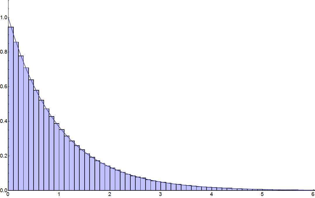 Figure 1
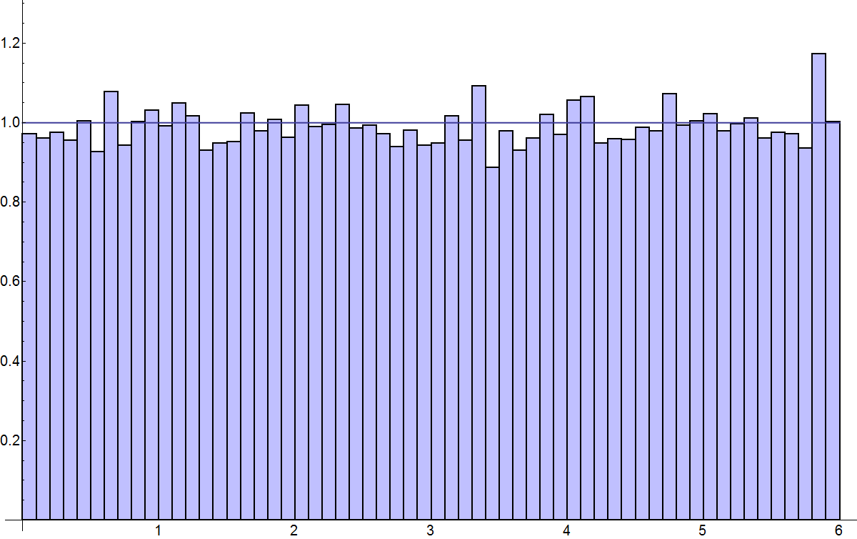 Figure 2
Peer Reviews
No public reviews on file for this paper yet. If you reviewed it on a platform where reviews are public (OpenReview, ICLR, NeurIPS, ICML), you can paste yours below so the community can read it here.
Videos
No videos yet. Explain this paper in a talk, walkthrough, or lecture? Add one.
Pair correlation for quadratic polynomials mod 1
Jens Marklof and Nadav Yesha
Jens Marklof, School of Mathematics, University of Bristol, Bristol BS8 1TW, U.K.
Nadav Yesha, School of Mathematics, University of Bristol, Bristol BS8 1TW, U.K. Department of Mathematics, King’s College London, Strand, London WC2R 2LS, U.K. [email protected]
(Date: March 18, 2024)
Abstract.
It is an open question whether the fractional parts of non-linear polynomials at integers have the same fine-scale statistics as a Poisson point process. Most results towards an affirmative answer have so far been restricted to almost sure convergence in the space of polynomials of a given degree. We will here provide explicit Diophantine conditions on the coefficients of polynomials of degree 2, under which the convergence of an averaged pair correlation density can be established. The limit is consistent with the Poisson distribution. Since quadratic polynomials at integers represent the energy levels of a class of integrable quantum systems, our findings provide further evidence for the Berry-Tabor conjecture in the theory of quantum chaos.
1. Introduction
Let be a polynomial of degree . In his ground-breaking 1916 paper [22], H. Weyl proved that, if one of the coefficients is irrational, then the sequence is uniformly distributed mod 1. That is, for any interval of length we have
[TABLE]
A century after Weyl’s work, it is remarkable how little is known on the fine-scale statistics of mod 1 in the case of polynomials of degree . (The linear case is singular and related to the famous three gap theorem; cf. [19, 2, 7, 14]). A popular example of such a statistics is the gap distribution: for given , order the values in mod 1, and label them as
[TABLE]
As we are working mod 1, it is convenient to set . The gap distribution of is then given by the probability measure defined, for any interval , by
[TABLE]
Rudnick and Sarnak [16] conjecture the following.
Conjecture 1.1**.**
Let . There is a set of full Lebesgue measure, such that for and any interval ,
[TABLE]
That is, the gap distribution of a degree polynomial with typical leading coefficient convergences to the distribution of waiting times of a Poisson process with intensity one. Sinai [18] pointed out that, for quadratic polynomials (with random coefficients), high moments of the fine-scale distribution do not converge; this is of course not in contradiction with Conjecture 1.1, which only concerns weak convergence. Pellegrinotti on the other hand pointed out that the first four moments do converge to the Poisson distribution [15].
The validity of Conjecture 1.1 is completely open. It is known that the conjecture cannot hold for every irrational . The general belief, however, is that includes every irrational number of Diophantine type , for any (see (1.10) below); this includes for instance all algebraic numbers [16]. The only result to-date on the gap distribution, due to Rudnick, Sarnak and Zaharescu [17], holds for quadratic polynomials, and establishes the convergence in (1.3) along subsequences for leading coefficients that are well approximable by rationals. Unfortunately, for these we cannot expect convergence along the full sequence, as they do not have the required Diophantine type.
A more accessible fine-scale statistics is the pair correlation measure which, for any bounded interval , is defined by
[TABLE]
Rudnick and Sarnak proved that the pair correlation measure of polynomials converges for almost every to Lebesgue measure, the pair correlation measure of a Poisson point process.
Theorem 1.2** (Rudnick-Sarnak [16]).**
Let . There is a set of full Lebesgue measure, such that for , , and any bounded interval ,
[TABLE]
It is currently not known whether any Diophantine condition on will guarantee the convergence in (1.5). In the quadratic case , Heath-Brown [8] gave an explicit construction of ’s such that (1.5) holds. The question whether (1.5) holds for Diophantine (which holds, e.g., for ), however, remains open to this day. See Truelsen [21] for a conditional result, and Marklof-Strömbergsson [13] for a derivation of (1.5) from a geometric equidistribution result. Boca and Zaharescu [3] generalized Theorem 1.2 to , where is any polynomial of degree with integer coefficients.
Zelditch proved an analogue of Theorem 1.2 for the sequence of polynomials
[TABLE]
where is a fixed polynomial satisfying on . Surprisingly, the pair correlation problem for seems harder than the case of fixed polynomials , and requires an additional Cesàro average:
Theorem 1.3** (Zelditch [23, add.]).**
There is a set of full Lebesgue measure, such that for , and any bounded interval ,
[TABLE]
Slightly weaker results hold when is only assumed to be a smooth function [23]. The motivation for the particular choice of is that the values represent the eigenphases of quantized maps [23]; the understanding of their statistical distribution is one of the central challenges in quantum chaos [1, 11]. Zelditch and Zworski have found analogous results for scattering phase shifts [24].
The aim of the present paper is to improve Theorem 1.3 for the specific example
[TABLE]
The corresponding triangular array , is uniformly distributed mod 1: For any bounded interval ,
[TABLE]
Appendix A comprises a precise bound on the discrepancy.
We will establish convergence of the pair correlation measure under an explicit Diophantine condition on , rather than convergence almost everywhere as in Theorem 1.3. Furthermore, we will shorten the Cesàro average and provide a power-saving in the rate of convergence.
An irrational is said to be Diophantine, if there exists such that
[TABLE]
for all . The constant is called the Diophantine type of ; by Dirichlet’s theorem, . Every quadratic surd, and more generally every with bounded continued fraction expansion, is of Diophantine type .
Theorem 1.4**.**
Choose as in (1.8), with Diophantine of type , and fix
[TABLE]
There exists such that for any bounded interval
[TABLE]
as (the implied constant in the remainder depends on ).
Theorem 1.4 extends to more general pair correlation measures, see Appendix B for a discussion. Numerical experiments (see Fig. 1.1) seem to suggest that the average over in (1.11) might in fact not be necessary in (1.11), and that furthermore the gap distribution is exponential (Fig. 1.2).
The proof of this statement reduces to a natural equidistribution theorem on a three-dimensional Heisenberg manifold, which we show derives from Strömbergsson’s recent quantitative Ratner equidistribution result on the space of affine lattices. Assuming that a more subtle equidistribution result holds (Conjecture 2.4), we can remove the average over in (1.11) and obtain the limit ; see Proposition 2.5.
The fact that is irrational and badly approximable is a crucial assumption. In the case , the gap distribution reduces to the distribution of spacing between quadratic residues mod , which was proved by Kurlberg and Rudnick [9] to be Poisson along odd, square-free and highly composite ’s.
If we do not insist on a rate of convergence, and also allow for a large average, Theorem 1.4 holds in fact for the more general polynomials
[TABLE]
where is Diophantine and arbitrary, or arbitrary and Diophantine. We will show in Appendix C that under these assumptions
[TABLE]
This statement is an immediate corollary of the quantitative Oppenheim conjecture for quadratic forms of signature , first proved by Eskin, Margulis and Mozes [6] for homogeneous forms, and generalized to inhomogeneous forms by Margulis and Mohammadi [10].
We conclude this introduction by briefly describing the relevance of our results to the theory of quantum chaos. The values for as in (1.8), or more generally (1.12), represent the eigenphases of a particularly simple quantum map studied by De Bièvre, Degli Esposti and Giachetti [4, §4B]: a quantized shear of a toroidal phase space with quasi-periodic boundary conditions, where quantifies the shear-strength and is related to the quasi-periodic boundary condition. Theorem 1.4 proves that the average two-point spectral statistics of this quantum map are Poisson.
The spacings in the sequence furthermore represent the quantum energy level spacings of a class of integrable Hamiltonian systems: a particle on a ring with quasi-periodic boundary condition (representing a magnetic flux line through its center), coupled to a harmonic oscillator. The corresponding energy levels are (in suitable units) , where , and . It is a short exercise to show that, after rescaling by , the energy levels have the same spacing statistics as for and . The index range is thus not as in (1.4); cf. Appendices B and C for the relevant generalizations.
Berry and Tabor [1] conjectured that typical integrable quantum systems should have Poisson statistics in the semiclassical limit , and the results presented in this study may therefore be viewed as further evidence for the truth of the Berry-Tabor conjecture. Other instances in which the conjecture could be rigorously established are reviewed in [11].
Acknowledgements
We thank Zeév Rudnick for helpful comments. The research leading to these results has received funding from the European Research Council under the European Union’s Seventh Framework Programme (FP/2007-2013) / ERC Grant Agreement n. 291147.
2. Outline of the proof: Smoothing and geometric equidistribution
We will first prove a smooth version of Theorem 1.4. Let be the Schwartz space of rapidly decreasing smooth functions on , equipped with the norms
[TABLE]
and denote
[TABLE]
the Fourier transform of , where we use the standard notation . For , define the smooth pair correlation function
[TABLE]
for technical reasons, introducing the shifts by inside in (2.1) gives a more convenient approximation to the sharp cutoff in (1.4).
Throughout the remainder of this paper we will use with as in (1.8), except for Appendix C where we consider general values of .
We prove the following smoothed variant of Theorem 1.4:
Theorem 2.1**.**
Fix a Diophantine of type , and let be fixed. There exist such that for any supported on and real valued and supported on ,
[TABLE]
as (the implied constant in the remainder depends on ).
(The specific choice of the interval in the above is simply for convenience. The proof generalizes to general bounded intervals.)
Define
[TABLE]
Theorem 2.1 will follow from the following proposition, which is key in this paper:
Proposition 2.2**.**
Fix a Diophantine of type , and let be fixed. There exist such that for any supported on and real valued and supported on ,
[TABLE]
as
The strategy of the proof of Proposition 2.2 which will be given in Section 5.3, is first to interpret the l.h.s. of (2.2) as a smooth sum of the absolute square of the Jacobi theta sum. Then we establish Proposition 2.2 from a geometric equidistribution result, which in turn follows from an effective Ratner equidistribution result due to Strömbergsson [20].
In order to give the exact formulation of our equidistribution result, let be the Haar measure on the Heisenberg group
[TABLE]
normalized such that it induces a probability measure on ; the latter is also denoted by .
Denote the differential operators
[TABLE]
For a compactly supported define the norm
[TABLE]
summing over all monomials in of degree .
Recall that a vector is called Diophantine of type , if there exists such that
[TABLE]
for all . By Dirichlet’s theorem, .
Proposition 2.3**.**
Fix a Diophantine vector of type , . Then for any compactly supported on and supported on , we have
[TABLE]
as , where are any integers that solve the equation .
To give the strategy behind the proof of Proposition 2.3, let be the semi-direct product Lie group with the multiplication law
[TABLE]
where the elements of are viewed as column vectors, and let be the subgroup . Denote
[TABLE]
We use the fact that, for every , the set
[TABLE]
is an embedding of as a submanifold of . By thickening this submanifold, we can use Strömbergsson’s result to obtain equidistribution of our points.
As for the pointwise limit of the pair correlation measure , we show in Appendix D that it also converges to the Lebesgue measure (and is thus consistent with the Poisson distribution), under the following equidistribution conjecture on the Heisenberg group , which is a pointwise version of Proposition 2.3 in the special case :
For define the norm
[TABLE]
summing over all monomials in the standard basis elements of the Lie algebra of (which correspond to left-invariant differential operators on ) of degree .
Conjecture 2.4**.**
There exist , such that for any fixed Diophantine of type there exists such that for any and supported on , we have
[TABLE]
as , where are any integers that solve the equation and is the Euler totient function.
We show in Appendix D:
Proposition 2.5**.**
Assuming Conjecture 2.4, there exists , such that for any fixed Diophantine of type , there exists such that for any bounded interval
[TABLE]
as
3. Background
3.1. Effective Ratner equidistribution theorem
Recall that is the semi-direct product Lie group with the multiplication law
[TABLE]
and that is the subgroup . Let be the Haar measure on , normalized such that it induces a probability measure on (also denoted by ).
Denote and , which are subgroups of and under the embedding . We will also use the following notations:
[TABLE]
as well as
[TABLE]
A key ingredient in our proof will be an effective Ratner equidistribution theorem due to Strömbergsson [20]. Let be the Lie algebra of , which may be identified with the space with the Lie bracket Fix the following basis of :
[TABLE]
We define the space of times continuously differentiable functions on such that for any left-invariant differential operator on of order , we have . For we define the norm
[TABLE]
summing over all monomials in , (which correspond to left-invariant differential operators on ) of degree .
We have the following formulation of Strömbergsson’s theorem:
Theorem 3.1** (Strömbergsson [20]).**
Let fixed, and let be a fixed Diophantine vector of type . Then for any supported on , and
[TABLE]
3.2. Jacobi theta sums
Recall the unique Iwasawa decomposition of a matrix :
[TABLE]
where , , and is the Poincaré half-plane model of the hyperbolic plane, which gives an identification with the left action of on given by
[TABLE]
For , let
[TABLE]
be the Jacobi Theta sum, where
[TABLE]
It is well-known that the operators are unitary; note that . Moreover, is a smooth function on (see [5] for example).
Let be the subgroup of defined by
[TABLE]
acting on by
[TABLE]
It is well-known (see [12, Proposition 4.9]) that is invariant under the left action of . Moreover, it is easy to see that
[TABLE]
We also have the following approximation for (see [12, Proposition 4.10]): For all
[TABLE]
where so that , , and the error term is uniform in .
4. The smooth pair correlation
function
In order to prove Proposition 2.2, we first notice that can be interpreted as a sum of , namely
[TABLE]
Next, we decompose into a sum over the divisors , and show that the contribution of large is small. We first recall the following lemma from [12]:
Lemma 4.1** (Marklof [12, Lemma 6.6]).**
Let be Diophantine of type , and be rapidly decreasing at , . Then, for any fixed and there exists such that
[TABLE]
uniformly for all , where (the implied constant is independent of ).
We will use Lemma 4.1 to prove the following lemma:
Lemma 4.2**.**
Fix a Diophantine of type , and let , be fixed. There exists such that for any supported on , real valued and supported on and ,
[TABLE]
as .
Proof.
Let , and assume first that is even. For , by the invariance of under we have
[TABLE]
where are (any) integers that solve the equation such that is even. By (4.2) and (3.4), for and for all we have
[TABLE]
where .
If is odd, then for , by the invariance of under we have
[TABLE]
where are (any) integers that solve the equation such that is even, and hence, for all we have
[TABLE]
Thus, for all there exists such that
[TABLE]
where
[TABLE]
To bound the main term, we divide the outer summation into three ranges: First, if , then we have , so by Lemma 4.1 we have
[TABLE]
and hence
[TABLE]
For we have so by Lemma 4.1,
[TABLE]
and then
[TABLE]
For we have , so by Lemma 4.1 for every there exists such that
[TABLE]
and hence for all there exists such that
[TABLE]
The lemma now follows from the bounds in the different ranges.
∎
We thus conclude that smooth averages of can be approximated by the following smooth sums of , which are closely related to the integral on the l.h.s. of (3.1), as we shall see in §5:
Corollary 4.3**.**
Fix a Diophantine of type , and let , , and be fixed. There exists such that for any supported on and real valued and supported on ,
[TABLE]
as
5. A geometric equidistribution result
5.1. Coordinates near the section
Let , and define the section
[TABLE]
In order to prove Proposition 2.3, given we define to be the following thickening of :
[TABLE]
so are local coordinates near the section .
Lemma 5.1**.**
Fix , and let . For any such that , we have
[TABLE]
Proof.
Let
[TABLE]
A short calculation yields that in the Iwasawa coordinates, has
[TABLE]
and likewise for we have . Therefore for any , and hence ∎
Recall that we identify elements of with elements of under the embedding . In particular and are identified with and respectively.
Let
[TABLE]
and
[TABLE]
Note that . Thus, for every ,
[TABLE]
is an embedding of as a submanifold of .
Let and . The proof of the next lemma is similar to the proof of Lemma 5.1:
Lemma 5.2**.**
Fix , and let . For any such that , we have
[TABLE]
The following key lemma shows that modulo , points on the lifted horocycle are in exactly when they are close to the points in Proposition 2.3 (under the embedding (5.1)) that we claim to be equidistributed:
Lemma 5.3**.**
Fix , and let . For any , we have
[TABLE]
if and only if where , and , and then
[TABLE]
where are any integers that solve the equation .
Proof.
For any , we have
[TABLE]
if and only if . Hence if and only if and .
Let . Then
[TABLE]
is in if and only if and . Moreover, and . Since the same calculation extends to , the statement of the lemma follows. ∎
5.2. Proof of Proposition 2.3
We will now use Theorem 3.1 to prove Proposition 2.3.
Proof.
Fix a Diophantine vector of type , . In addition, fix , and fix supported on such that . Let , supported on and supported on .
Recalling the embedding (5.1), we define
[TABLE]
and let be defined by
[TABLE]
Note that by Lemma 5.2, all but one of the terms in (5.2) vanish, so is well-defined.
We have
[TABLE]
Note that since and , intervals of the form are disjoint for . Thus, by Lemma 5.3,
[TABLE]
In terms of the Iwasawa coordinates (Section 3.2), the measure is given by
[TABLE]
Therefore,
[TABLE]
Making the change of variables , , for which the Jacobian is equal to
[TABLE]
so that
[TABLE]
we get (using the fact that is of unit mass) that
[TABLE]
Thus, by Theorem 3.1,
[TABLE]
Finally, we note that in the coordinates of
[TABLE]
and therefore (Since and are fixed) . Note that equation (5.3) also holds with on the l.h.s. instead of , since we can replace the function with , leaving the r.h.s. of (5.3) unchanged. Hence, the statement of the proposition follows. ∎
5.3. Proof of Proposition 2.2
Proof.
By the invariance of under and since for any we have , we see that the function
[TABLE]
belongs to , i.e., for every , we have
[TABLE]
In particular, is invariant under , and therefore for fixed , the function
[TABLE]
belongs to , and by (3.3)
[TABLE]
Moreover, by the same reasoning of (3.4), for
[TABLE]
where so that ; for all , there exists such that and all its partial derivatives of order are uniformly bounded by . Fix and let
[TABLE]
Since is supported on and , vanishes unless
[TABLE]
and in particular it vanishes unless , so is compactly supported on . If and are integers that solve the equation , then by (5.4),
[TABLE]
Thus,
[TABLE]
where are any integers that solve the equation .
By Proposition 2.3 (applied with ; recall the remark in the end of the proof of Proposition 2.3), the right hand side of (5.6) is equal to
[TABLE]
The main term is equal to
[TABLE]
On the other hand, Thus,
[TABLE]
Recalling Corollary 4.3, Proposition 2.2 now follows from the condition , assuming is chosen sufficiently small. ∎
6. Proof of the main theorems
We are now able to prove the main theorems using Proposition 2.2.
6.1. Proof of Theorem 2.1
Proof.
Fix . By Proposition 2.2, there exist such that for for any supported on and real valued and supported on ,
[TABLE]
as By Poisson summation formula,
[TABLE]
Note that
[TABLE]
and
[TABLE]
Theorem 2.1 now follows by substituting (6.1), (6.3) and (6.4), into (6.2). ∎
6.2. Proof of Theorem 1.4
Proof.
Fix . By Theorem 2.1, there exist such that for any supported on and real valued and supported on ,
[TABLE]
as .
Fix a bounded interval and denote by its characteristic function. Given , we can find smooth functions such that:
- (i)
are supported in 2. (ii)
. 3. (iii)
4. (iv)
5. (v)
The derivative of any order of is uniformly bounded.
See [12, §8] for a detailed construction.
Let , and choose to be a smooth approximation to the characteristic function on the interval such that:
- (i)
2. (ii)
in . 3. (iii)
in the complement of . 4. (iv)
for the -th derivative . 5. (v)
the following inequalities hold:
[TABLE]
Note that , , and are all of the form
By (6.5),
[TABLE]
and Theorem 1.4 follows with by choosing , and . ∎
Appendix A Uniform distribution mod 1 of
We show that is uniformly distributed mod (for any ), and give an explicit rate of decay (uniform in ) for its discrepancy
[TABLE]
Proposition A.1**.**
We have
[TABLE]
where is the divisor function, and the implied constant is independent of .
Proof.
By Erdős–Turán inequality, there exists a constant such that for every integer
[TABLE]
By Weyl differencing,
[TABLE]
The inner sum of (A.1) is equal to whenever ; otherwise it is equal to . It follows that
[TABLE]
We have
[TABLE]
and therefore
[TABLE]
choosing .∎
Appendix B More general pair correlation functions
We consider slightly more general pair correlation measures, which also consider a general truncation of the indices : For bounded intervals set
[TABLE]
Our original pair correlation measure (1.4) is recovered by setting . We have the following generalization of Theorem 1.4:
Theorem B.1**.**
Choose as in (1.8), with Diophantine of type , and fix
[TABLE]
There exists such that for any bounded intervals
[TABLE]
as (the implied constant in the remainder depends on and ).
By the same approximation arguments of Section 6 (since the scale of the approximation is larger than ), Theorem B.1 also holds if we add shifts to the summation range in (B.1), i.e., if we define
[TABLE]
The proof of Theorem B.1 goes along similar lines of the proof of Theorem 1.4. First, for we define a more general, unequally weighted smooth pair correlation function:
[TABLE]
Note that the properties of Section 3.2 regarding the absolute square of the Jacobi theta sum hold in fact more generally for where (see [12]), i.e., is invariant under the left action of ; we have
[TABLE]
and for all ,
[TABLE]
where , and the error term is uniform in .
Thus, the generalization of Theorem 2.1 to the more general smooth pair correlation functions (B.3) is straightforward.
Theorem B.2**.**
Under the assumptions of Theorem 2.1, where in addition are real valued and compactly supported,
[TABLE]
as (the implied constant in the remainder depends on and the supports of ).
Theorem B.1 follows by the same approximation arguments of Section 6.
Appendix C Long averages
We show in this appendix that averages of over long intervals have Poisson statistics for the sequence assuming either or is Diophantine. This follows from the quantitative version of the Oppenheim conjecture for quadratic forms of signature [6, 10].
We work with the general pair correlation measure (B.1) introduced in Appendix B; the same argument will also work for the pair correlation measure (B.2).
Theorem C.1**.**
Fix such that and either or is Diophantine. If , then for any bounded intervals
[TABLE]
If , then the above holds provided .
In particular, Theorem C.1 holds for a Diophantine and .
Proof.
Define the signature quadratic form
[TABLE]
Let and define
Note that
[TABLE]
Let
[TABLE]
Then
[TABLE]
Since either or is Diophantine, the form is Diophantine (recall [10, Definition 1.8]). Moreover, let with , and . If , then belongs to an exceptional subspace of if and only if . If , then belongs to an exceptional subspace of if and only if or ; since in that case we assume that , the condition can only occur for a bounded number of whose contribution to the sum is .
Since for any and the set
[TABLE]
can be written as a difference of two star-shaped regions, we deduce from [10, Theorem 1.9] using a standard approximation argument that
[TABLE]
∎
Appendix D Conjecture 2.4 implies is Poisson
We show in this appendix that, assuming Conjecture 2.4, the pair correlation measure converges weakly to Lebesgue measure (without averaging on ).
D.1. Proof of Proposition 2.5
Proof.
By an approximation argument similar to that of §6, it is enough to show that there exist , such that for any Diophantine of type , there exist such that for any supported on , real valued and supported on ,
[TABLE]
as .
To prove (D.1), recall that by Lemma 4.2, for and for , there exists such that for any supported on , real valued and supported on ,
[TABLE]
as .
In addition,
[TABLE]
where are (any) integers that solve the equation . Assuming conjecture 2.4, there exist , such that for any Diophantine of type , there exists such that the r.h.s. of (D.2) is equal to
[TABLE]
Since
[TABLE]
we have
[TABLE]
By (5.5), there exists such that that Thus we conclude that (D.3) is equal to
[TABLE]
and taking sufficiently small, Proposition 2.5 follows.∎
The reference list from the paper itself. Each links out to its DOI / PubMed record.
- 1[1] M. V. Berry and M. Tabor, Level clustering in the regular spectrum . Proc. Roy. Soc. A. 356 (1977), 375–394.
- 2[2] P. M. Bleher, The energy level spacing for two harmonic oscillators with generic ratio of frequencies . J. Statist. Phys. 63 (1991), no. 1-2, 261–283.
- 3[3] F. P. Boca and A. Zaharescu, Pair correlation of values of rational functions (mod p 𝑝 p ) . Duke Math. J. 105 (2000), no. 2, 267–307.
- 4[4] S. De Bièvre, M. Degli Esposti and R. Giachetti, Quantization of a class of piecewise affine transformations on the torus . Comm. Math. Phys. 176 (1996), no. 1, 73–94.
- 5[5] F. Cellarosi and J. Marklof, Quadratic Weyl sums, automorphic functions, and invariance principles . Proceedings of the London Mathematical Society. 113 (2016), no. 6, 775–828.
- 6[6] A. Eskin, G. Margulis and S. Mozes, Quadratic forms of signature ( 2 , 2 ) 2 2 (2,2) and eigenvalue spacings on rectangular 2 2 2 -tori . Ann. of Math. (2) 161 (2005), no. 2, 679–725.
- 7[7] C. D. Greenman, The generic spacing distribution of the two-dimensional harmonic oscillator . J. Phys. A. 29 (1996), no. 14, 4065–4081.
- 8[8] D. R. Heath-Brown, Pair correlation for fractional parts of α n 2 𝛼 superscript 𝑛 2 \alpha n^{2} . Math. Proc. Cambridge Philos. Soc. 148 (2010), no. 3, 385–407.