Onsager's conjecture for admissible weak solutions
Tristan Buckmaster, Camillo De Lellis, L\'aszl\'o Sz\'ekelyhidi Jr.,, Vlad Vicol

TL;DR
This paper proves the existence of weak solutions to the 3D Euler equations with prescribed energy profiles and regularity below 1/3, demonstrating a form of the Onsager conjecture and an h-principle in this regime.
Contribution
It establishes the existence of energy-prescribed weak solutions with Hölder regularity less than 1/3 and shows a corresponding h-principle, extending Onsager's conjecture.
Findings
Existence of weak solutions with Hölder regularity < 1/3
Solutions can match arbitrary smooth energy profiles
A form of the h-principle holds in the subcritical regularity class
Abstract
We prove that given any , a time interval , and given any smooth energy profile , there exists a weak solution of the three-dimensional Euler equations such that , with for all . Moreover, we show that a suitable -principle holds in the regularity class , for any . The implication of this is that the dissipative solutions we construct are in a sense typical in the appropriate space of subsolutions as opposed to just isolated examples.
Click any figure to enlarge with its caption.
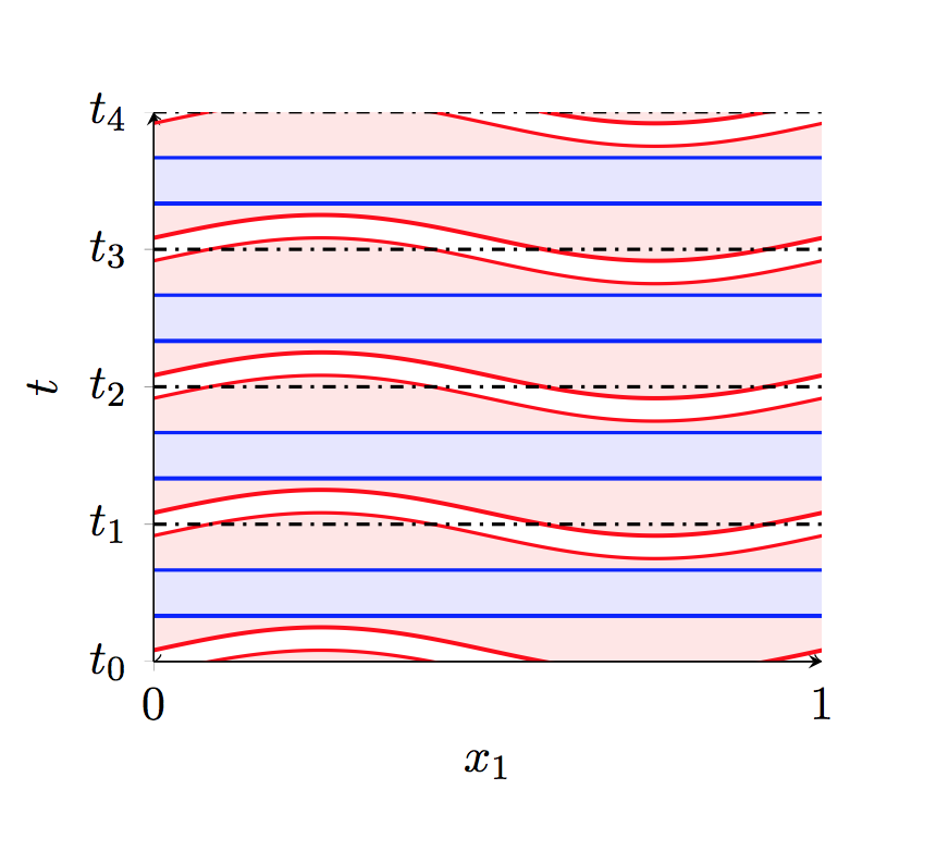 Figure 1
Peer Reviews
No public reviews on file for this paper yet. If you reviewed it on a platform where reviews are public (OpenReview, ICLR, NeurIPS, ICML), you can paste yours below so the community can read it here.
Videos
No videos yet. Explain this paper in a talk, walkthrough, or lecture? Add one.
Onsager’s conjecture for admissible weak solutions
Tristan Buckmaster
Courant Insitute of Mathematical Sciences, New York University, New York, NY 10012, USA
,
Camillo De Lellis
Institut für Mathematik, Universität Zürich, CH-8057 Zürich, Switzerland
,
László Székelyhidi Jr
Institut für Mathematik, Universität Leipzig, D-04103 Leipzig, Germany
and
Vlad Vicol
Department of Mathematics, Princeton University, Princeton, NJ 08544, USA
Abstract.
We prove that given any , a time interval , and given any smooth energy profile , there exists a weak solution of the three-dimensional Euler equations such that , with for all . Moreover, we show that a suitable -principle holds in the regularity class , for any . The implication of this is that the dissipative solutions we construct are in a sense typical in the appropriate space of subsolutions as opposed to just isolated examples.
1. Introduction
In this paper we consider the incompressible Euler equations
[TABLE]
in the periodic setting , where is a vector field representing the velocity of the fluid and is the pressure. We study weak (distributional) solutions which are Hölder continuous in space, i.e. such that111The smallest constant satisfying (1.2) will be denoted by , cf. Appendix A. We will write when is Hölder continuous in the whole space-time.
[TABLE]
for some constant which is independent of time .
In his famous 1949 note on statistical hydrodynamics Lars Onsager [Ons49] conjectured that the threshold regularity for the validity of the energy conservation of weak solutions of (1.1) is the exponent : in particular he asserted that for larger Hölder exponents any weak solution would conserve the energy, whereas for any smaller exponent there are solutions which do not. The first assertion was fully proved by Constantin, E and Titi in [CET94], after a partial result of Eyink in [Eyi94] (see also [CCFS08] for a sharper criterion in -based spaces). Concerning the second assertion, the first proof of the existence of a square summable weak solution which does not preserve the energy is due to Scheffer in his pioneering paper [Sch93]. A different proof has been later given by Shnirelman in [Shn97]. In [DLS09] the second and third author realized that techniques from the theory of differential inclusions could be applied very efficiently to produce bounded weak solutions which violate the energy conservation in several forms. Pushed by the analogy of these constructions with the famous solutions of Nash and Kuiper for the isometric embedding problem (cf. [Nas54] and [Kui55]) they proposed to approach the remaining statement of the Onsager’s conjecture in a similar way (cf. [DLS12]). Indeed in [DLS13] and [DLS14] they were able to give the first examples of, respectively, continuous and Hölder continuous solutions which dissipate the energy, reaching the threshold exponent . After a series of important partial results improving the threshold and the techniques from several points of view, cf. [Ise13a, BDLS13, BDLISJ15, Buc15, BDLS16], in his recent paper Isett [Ise16] has been able to finally reach the Onsager exponent . The proof of Isett combines previous ideas with two new important ingredients, one developed by Daneri and the third author in [DSJ16] (the introduction of Mikado flows, see Section 2.6) and one introduced by Isett himself the aforementioned paper (the gluing technique, see Section 2.5).
However, the solutions produced in [Ise16] are only shown to be nonconservative and in fact for those solutions the total kinetic energy fails to be monotonic on any interval of time. Thus Isett’s theorem left open the question whether it is possible or not to construct solutions which dissipate the kinetic energy (i.e. with strictly monotonic decreasing energy). In fact the latter is a relevant point, for at least two reasons: first of all because dissipative solutions satisfy the weak-strong uniqueness property [Lio96, BDLS11] and secondly because indeed Onsager in his work conjectures the existence of dissipative solutions. Indeed, in [Ons49] Onsager states:
It is of some interest to note that in principle, turbulent dissipation as described could take place just as readily without the final assistance by viscosity.
In this note we suitably modify the approach of Isett in order to show the following theorem.
Theorem 1.1**.**
Assume is a strictly positive smooth function. Then for any there exists a weak solution to (1.1) such that
[TABLE]
We are indeed able to prove a stronger statement than Theorem 1.1, namely an -principle in the sense of [DSJ16]. Following [DSJ16] we introduce smooth strict subsolutions of the Euler equations.
Definition 1.2**.**
A smooth strict subsolution of (1.1) on is a smooth triple with a symmetric -tensor, such that
[TABLE]
and is positive definite for all .
We then can prove that any smooth strict subsolution can be suitably approximated by solutions for any . More precisely
Theorem 1.3**.**
Let be a smooth strict subsolution of the Euler equations on and let . Then there exists a sequence of weak solutions of (1.1) such that ,
[TABLE]
uniformly in time, and furthermore for all
[TABLE]
Theorem 1.1 can be concluded as a simple corollary of Theorem 1.3. However we give an alternative simpler and self-contained argument for Theorem 1.1: indeed the proof of Theorem 1.3 invokes some results of [DSJ16], whereas the argument for Theorem 1.1 is entirely contained in our note, aside from technical propositions which are classical statements in the literature, all collected in the Appendix.
The most important differences in our proof compared to that of [Ise16] rely on the estimates for the “gluing step” of Isett’s proof (we refer to Section 2.5 for more details) and in a simple remark concerning the regions where the perturbation is added (see Section 2.6). We note that, even without the extra benefit of imposing the energy profile and achieving the most general -principle statement, the proof proposed here is considerably shorter than that of [Ise16].
Acknowledgments
The work of T.B. has been partially supported by the National Science Foundation grant DMS-1600868. The research of C.D.L. has been supported by the grant 200021159403 of the Swiss National Foundation. L.Sz. gratefully acknowledges the support of the ERC Grant Agreement No. 277993. V.V. was partially supported by the National Science Foundation grant DMS-1514771 and by an Alfred P. Sloan Research Fellowship.
2. Outline of the proof
As already mentioned, although Theorem 1.1 can be recovered as a corollary of Theorem 1.3, in this section we outline an independent proof, reducing it to a suitable iterative procedure, summarized in Proposition 2.1 below. The same iteration procedure can be used to prove Theorem 1.3, as shown in Section 7 at the end of the note, but the corresponding argument we will need some results from [DSJ16], which we state without proof. In contrast, the proof of Theorem 1.1 is completely self-contained.
2.1. Inductive proposition
First of all, we impose for the moment that
[TABLE]
(we will see later that this can be done without loosing generality).
Let then be a natural number. At a given step we assume to have a triple to the Euler-Reynolds system (1.3), namely such that
[TABLE]
to which we add the constraints that
[TABLE]
and that
[TABLE]
(which uniquely determines the pressure).
The size of the approximate solution and the error will be measured by a frequency and an amplitude , which are given by
[TABLE]
where denotes the smallest integer , is a large parameter, is close to and is the exponent of Theorem 1.1. The parameters and are then related to .
We proceed by induction, assuming the estimates
[TABLE]
where is a small parameter to be chosen suitably (which will depend upon ), and is a universal constant (which is fixed throughout the iteration and whose choice depends on certain geometric properties of the space of symmetric matrices and on the “squiggling” regions of the perturbation step, cf. Remark 5.2, Lemma 5.5 and Definition 5.6). We refer to Appendix A for the definitions of the Hölder norms used above, where we take into account only space regularity.
Proposition 2.1**.**
There is a universal constant with the following property. Assume and
[TABLE]
Then there exists an depending on and , such that for any there exists an depending on , , and , such that for any the following holds: Given a strictly positive energy function satisfying (2.1), and a triple solving (2.2)-(2.4) and satisfying the estimates (2.7)–(2.10), then there exists a solution to (2.2)-(2.4) satisfying (2.7)–(2.10) with replaced by . Moreover, we have
[TABLE]
The proof of Proposition 2.1 is summarized in the Sections 2.3, 2.4, 2.5 and 2.6, but its details will occupy most of the paper and will be completed in Section 6 below. We show next that this proposition immediately implies Theorem 1.1.
2.2. Proof of Theorem 1.1
First of all, we fix any Hölder exponent and also the parameters and , the first satisfying (2.11) and the second smaller than the threshold given in Proposition 2.1. Next we show that, without loss of generality, we may further assume the energy profile satisfies
[TABLE]
provided the parameter is chosen sufficiently large.
To see this, we first note that the Euler equations are invariant under the transformation
[TABLE]
Thus if we choose
[TABLE]
then using the scaling invariance, the stated problem reduces to finding a solution with the energy profile given by
[TABLE]
for which we have
[TABLE]
If is chosen sufficiently large then we can ensure
[TABLE]
Now we apply Proposition 2.1 iteratively with . Indeed the pair trivially satisfies (2.7)–(2.9), whereas the estimate (2.10) and (2.1) follows as a consequence of (2.13). Notice that by (2.12) converges uniformly to some continuous . Moreover, we recall that the pressure is determined by
[TABLE]
and (2.4) and thus is also converging to some pressure (for the moment only in for every ). Since uniformly, the pair solves the Euler equations.
Observe that using (2.12) we also infer222Throughout the manuscript we use the the notation to denote , for a sufficiently large constant , which is independent of , and , but may change from line to line.
[TABLE]
and hence that is uniformly bounded in for all . To recover the time regularity, we could use the Euler equations and the general result in [Ise13b]. Nevertheless, we believe that the following short and self-contained proof of the time-regularity may be of independent interest:
Fix a smooth standard mollifier in space, let , and consider , where . From standard mollification estimates we have
[TABLE]
and thus uniformly as . Moreover, obeys the following equation
[TABLE]
Next, since
[TABLE]
using Schauder’s estimates, for any fixed we get
[TABLE]
(where the constant in the estimate depends on but not on ). Similarly,
[TABLE]
Thus the above estimates yield
[TABLE]
Next, for we conclude from (2.15) and (2.16) that
[TABLE]
Here we have chosen sufficiently small (in terms of and ) so that that . Thus, the series
[TABLE]
converges in . Since we already know , we obtain that as desired, with arbitrary.
Finally, since as , from (2.10) we have
[TABLE]
which completes the proof of the theorem.
2.3. Stages
Except for Section 7, the rest of the paper is devoted to the proof of Proposition 2.1. It will be useful to make the assumption that is small enough so to have
[TABLE]
which also require that is large enough to absorb any constant appearing from the ratio , for which we have the elementary bounds
[TABLE]
The proof consists of three stages, in each of which we modify . Roughly speaking, the stages are as follows:
- •
Mollification: ;
- •
Gluing: ;
- •
Perturbation: .
2.4. Mollification step
The first stage is mollification: we mollify at length scale in order to handle the loss of derivative problem, typical of convex integration schemes. To this aim, we fix a standard mollification kernel in space and introduce the mollification parameter
[TABLE]
and define
[TABLE]
where is the traceless part of the tensor . These functions obey the equation
[TABLE]
in view of (2.2).
Observe, again choosing sufficiently small and sufficiently large we can assume
[TABLE]
which will be applied repeatedly in order to simplify the statements of several estimates.
From (2.21), standard mollification estimates and Proposition A.2 we obtain the following bounds333In the following, when considering higher order norms or , the symbol will imply that the constant in the inequality might also depend on .
Proposition 2.2**.**
[TABLE]
Proof of Proposition 2.2.
The bounds (2.22) and (2.23) follow from the obvious estimates
[TABLE]
and
[TABLE]
Next, applying Proposition A.2,
[TABLE]
on the other hand, by (2.21) , from which (2.24) follows. Similarly, by Proposition A.2,
[TABLE]
which implies (2.25). ∎
2.5. Gluing step
In the second stage we encounter the new crucial ingredient introduced by Isett in [Ise16]: we glue together exact solutions to the Euler equations in order to produce a new , close to , whose associated Reynolds stress error has support in pairwise disjoint temporal regions of length in time, where
[TABLE]
The parameter should be compared to the parameter used in the paper [BDLISJ15]. Indeed, satisfies precisely the same parameter inequalities that satisfies in Section 2 of [BDLISJ15]. We note in particular that like in [BDLISJ15] we have the CFL-like condition
[TABLE]
as long as is sufficiently large.
More precisely, we aim to construct a new triple solving the Euler Reynolds equation (2.2) such that the temporal support of is contained in pairwise disjoint intervals of length and such that the gaps between neighbouring intervals is also of length . More precisely, for any let
[TABLE]
We require
[TABLE]
Moreover, will satisfy the following estimates for any
[TABLE]
where the implicit constants depend only on , and , cf. Propositions 4.2, 4.3 and 4.4.
The gluing procedure will be broken up into two parts: first, we construct a sequence of exact solutions to the Euler equations with appropriate stability estimates in Section 3 and then we glue the solutions together in Section 4 with a partition of unity in order to construct satisfying the properties mentioned above. This is indeed the key idea of Isett in [Ise16]. The main difference with [Ise16] is in the construction of the tensor : in this paper we use the usual elliptic operators introduced in [DLS13]. This has the advantage that our Reynolds stress remains trace free, in contrast to the one of [Ise16], and in turn this is crucial to control the energy in the perturbation step below. It should be noticed that in [Ise16] the author resorts to a different definition of because he is not able to find efficient estimates. Our main technical improvement is that this difficulty can be overcome employing suitable commutator estimates on the advective derivative of differential operators of negative order, cf. the proof of Proposition 3.4 and Proposition D.1. This remark allows us not only to keep a better control on the energy and a trace-free Reynolds stress with the desired estimate, but it also shortens the arguments considerably compared to [Ise16].
2.6. Perturbation and proof of Proposition 2.1
The gluing procedure can be used to localize the Reynolds stress error to small disjoint temporal regions, but it cannot be used to completely eliminate the error.
First of all note that as a corollary of (2.10), (2.25) and (2.33), by choosing sufficiently large we can ensure that
[TABLE]
Starting with the solution satisfying (2.28) and the estimates (2.29)-(2.34), we then produce a new solution of the Euler-Reynolds system (2.2) with estimates
[TABLE]
cf. Corollary 5.8 and Propositions 6.1 and 6.2.
As in previous papers [DLS14, Ise13a, BDLS13, BDLISJ15, BDLS16] the key idea, introduced in [DLS13], for reducing the size of the error is to add a highly oscillatory perturbation to . Previous schemes heavily relied on Beltrami flows, but these seemed insufficient to push the method beyond Hölder exponent . A new set of flows, called Mikado flows, with much better properties were introduced in [DSJ16] and indeed, a key element in the proof of Isett [Ise16] is the observation, already used in [DSJ16], that Mikado flows behave better under advection by a mean flow.
An important point is that the Mikado flows will not only be used to “cancel” the error , but also to “improve the energy” in areas where the error vanishes identically. In particular, the perturbation will be added in spacetime regions which are disjoint and contained in time-slabs of thickness , but with the property that their projections on the time axis is a covering of the interval .
Proof of Proposition 2.1.
The estimate (2.12) is a consequence of (2.22), (2.23), (2.29), (2.30) and (2.35):
[TABLE]
where the constant depends on , but not on and . In particular, for every fixed (2.12) holds if is large enough. For (2.8), we use the induction assumption to get
[TABLE]
and again a sufficiently large choice of will guarantee . Similarly for (2.9), which will follow from
[TABLE]
From (2.36) and (2.37), the inequalities (2.7) and (2.10) follow as a consequence of the parameter inequality
[TABLE]
To see this, one divides by the right hand side, takes logarithms and divides by , to obtain
[TABLE]
where the error term is due to the constants in (2.18). From the relation (2.11), if is sufficiently small we obtain
[TABLE]
Hence fixing to satisfy (2.11), choosing subsequently sufficiently small and then sufficiently large, we obtain (2.38).
Finally, an entirely analogous argument shows (2.10) from (2.37). ∎
3. Stability estimates for classical exact solutions
3.1. Classical solutions
For each , let , and consider smooth solutions of the Euler equations
[TABLE]
defined over their own maximal interval of existence. Next, recall the following
Proposition 3.1**.**
For any there exists a constant with the following property. Given any initial data , and , there exists a unique solution to the Euler equation
[TABLE]
Moreover, obeys the bounds
[TABLE]
for all , where the implicit constant depends on and .
Proof of Proposition 3.1.
The proof of the existence of a unique solution is standard (see e.g. [MB02, Chapter 4]), and follows from the restriction . The higher-order bounds (3.2) are also standard, and can be obtained as follows: For any multi-index with we have
[TABLE]
Using the equation for the pressure and Schauder estimates we obtain
[TABLE]
Therefore
[TABLE]
and (3.2) follows by applying (B.3) and Grönwall’s inequality. ∎
An immediate consequence is:
Corollary 3.2**.**
If is sufficiently large, for , we have
[TABLE]
Proof of Corollary 3.2.
We apply Proposition 3.1 and use the estimate (2.27) to obtain
[TABLE]
for any . From (2.23) we then deduce the estimate (3.3). ∎
3.2. Stability and estimates on
We will now show that for , is close to and by the identity
[TABLE]
the vector field is also close to .
Proposition 3.3**.**
For and we have
[TABLE]
where we write
[TABLE]
for the transport derivative.
Proof of Proposition 3.3.
Let us first consider (3.4) with . From (2.20) and (3.1) we have
[TABLE]
In particular, using
[TABLE]
estimates (2.24) and (3.3), and Proposition C.1 (recall that is given by a Calderón-Zygmund operator), we conclude
[TABLE]
Thus, using (2.24) and the definition of , we have
[TABLE]
By applying (B.3) we obtain
[TABLE]
Applying Grönwall’s inequality and using the assumption we obtain
[TABLE]
i.e. (3.4) for the case . Then, as a consequence of (3.10) we obtain (3.6) for the case .
Next, consider the case and let be a multiindex with . Commuting the derivative with the material derivative we have
[TABLE]
where in the last inequality we used the standard interpolation inequalities on Hölder norms, cf. (A.1). On the other hand differentiating (3.8) leads to
[TABLE]
where we have used (3.11). Furthermore, from (3.9) we also obtain, using Corollary 3.2 and (3.11)
[TABLE]
Summarizing, for any multiindex with we obtain
[TABLE]
Therefore, invoking once more (B.3) we deduce
[TABLE]
and hence, using Grönwall’s inequality and the assumption we obtain (3.4). From (3.13) and (3.12) we then also conclude (3.5) and (3.6). ∎
3.3. Estimates on vector potentials
Define the vector potentials to the solutions as
[TABLE]
where is the Biot-Savart operator, so that
[TABLE]
Our aim is to obtain estimates for the differences . The heuristic is as follows: from Proposition 3.3 we obtain
[TABLE]
Since the characteristic length-scale of the vectorfields is (cf. Corollary 3.2), we expect to gain a factor when passing to first order potentials. This is formalized in Proposition 3.4 below.
Proposition 3.4**.**
For , we have that
[TABLE]
where is as in (3.7).
Proof of Proposition 3.4.
Set and observ that . Hence, it suffices to estimate in place of .
The estimate on for follows directly from (3.4) and the fact that is a bounded operator on Hölder spaces:
[TABLE]
Next, observe that
[TABLE]
Since with , we have444Here we use the notation for vector fields .
[TABLE]
so that we can write (3.19) as
[TABLE]
Taking the curl of (3.20) the pressure term drops out. Using in addition that and the identity , we then arrive at
[TABLE]
where
[TABLE]
Consequently,
[TABLE]
Setting and using (B.3) and Grönwall’s inequality we obtain
[TABLE]
which together with (3.18) gives (3.16). Using (3.16) into (3.21) we conclude
[TABLE]
Finally commuting the derivatives in the -norm with as in the proof of Proposition 3.3 and using again (3.16) we achieve (3.17). ∎
4. Gluing procedure
Now we proceed to glue the solutions together in order to construct . The stability estimates above will be used in order to ensure that remains an approximate solution to the Euler equations.
4.1. Partition of unity and definition of
Let
[TABLE]
Note that is a decomposition of into pairwise disjoint intervals. We define a partition of unity in time with the following properties:
- •
The cut-offs form a partition of unity
[TABLE]
- •
and moreover
[TABLE]
- •
For any and we have
[TABLE]
We define
[TABLE]
Observe that . Furthermore, if , then and for , therefore on :
[TABLE]
and
[TABLE]
On the other hand, if then and for all for all sufficiently close to (since is open). Then for all we have
[TABLE]
and, from (3.1),
[TABLE]
4.2. The new Reynods tensor
In order to define the new Reynolds tensor, we recall the operator from [DLS13], which can be thought of as an “inverse divergence” operator for symmetric tracefree 2-tensors. The operator is defined as
[TABLE]
when acting on vectors with zero mean on . The following statement, taken from [DLS13], can be proved by direct calculation.
Proposition 4.1**.**
The tensor defined in (4.4) is symmetric, and we have
[TABLE]
for any with zero mean on .
We define
[TABLE]
for and , for . Furthermore, we set
[TABLE]
It follows from the preceding discussion and Proposition 4.1 that
- •
is a smooth symmetric and traceless 2-tensor;
- •
For all
[TABLE]
- •
.
4.3. Estimates on
Next, we estimate the various Hölder norms of and in order to obtain (2.29)-(2.32).
Proposition 4.2**.**
The velocity field satisfies the following estimates
[TABLE]
for all .
In particular, this lemma shows that the claimed estimates (2.29)–(2.30) indeed hold.
Proof of Proposition 4.2.
By definition
[TABLE]
Therefore Proposition 3.3 implies
[TABLE]
Note that using the definition of in (2.19) and in (2.26) and the comparison (2.21)
[TABLE]
Therefore we obtain (4.5), and furthermore, for any
[TABLE]
Then it also follows using (2.23) that
[TABLE]
4.4. Estimates on the stress tensor
We are now in a position to estimate the glued stress tensor :
Proposition 4.3**.**
The stress tensor satisfies the following bounds for any :
[TABLE]
This shows that the claimed estimates (2.31)–(2.32) are indeed obeyed by .
Proof of Proposition 4.3.
Recall that , so that we may write for :
[TABLE]
Note that is a zero-order operator. Therefore we obtain from Propositions 3.3 and 3.4 for any with
[TABLE]
Here we used again (4.9). Next, we calculate
[TABLE]
where denotes the commutator. Hence, using Proposition D.1 and Propositions 3.3 and 3.4 we deduce
[TABLE]
Finally, we deduce using (4.6):
[TABLE]
again using (4.9). ∎
To finish this section we show that has approximately the same energy as :
Proposition 4.4**.**
The difference of the energies of and satisfies
[TABLE]
Proof of Proposition 4.4.
Observe that for
[TABLE]
so that, taking the trace:
[TABLE]
Next, recall that and are smooth solutions of (3.1) and (2.20) respectively, therefore
[TABLE]
where we have used (2.24) and (3.3). Moreover, for . Therefore, after integrating in time we deduce
[TABLE]
Furthermore, using (3.4) and (4.9)
[TABLE]
Therefore
[TABLE]
which concludes the proof. ∎
5. Perturbation step
In this section, we will outline the construction of the perturbation , where
[TABLE]
As already explained in the outline of the proof, the perturbation is highly oscillatory and will be based on the Mikado flows introduced in [DSJ16], which are designed to cancel the low frequency error and are Lie-advected by the mean flow of .
5.1. Mikado flows
We begin by recalling the construction of Mikado flows given in [DSJ16].
Lemma 5.1**.**
For any compact subset there exists a smooth vector field
[TABLE]
such that, for every
[TABLE]
and
[TABLE]
Using the fact that is -periodic and has zero mean in , we write
[TABLE]
for some coefficients and complex vector , satisfying and . From the smoothness of , we further infer
[TABLE]
for some constant , which depends, as highlighted in the statement, on , and .
Remark 5.2**.**
Later in the proof the estimates (5.5) will be used with a specific choice of the compact set and of the integers and : this specific choice will then determine the universal constant appearing in Proposition 2.1.
Using the Fourier representation we see that from (5.3)
[TABLE]
where
[TABLE]
for any .
It will also be useful to write the Mikado flows in terms of a potential. We note
[TABLE]
5.2. Squiggling stripes and the stress tensor
Recall that is supported in the set , whereas, from (4.2) it follows that , where the open intervals have length each, except for the first and last one, which might be shortened by the intersection with , more precisely
[TABLE]
We start by defining smooth non-negative cut-off functions with the following properties
- (i)
with for all ; 2. (ii)
for ; 3. (iii)
; 4. (iv)
; 5. (v)
There exists a positive geometric constant such that for any
[TABLE]
In view of (iv) we set
[TABLE]
Lemma 5.3**.**
There exists cut-off functions with the properties (i)-(v) above and such that for any and
[TABLE]
where are geometric constants depending only upon and .
Proof of Lemma 5.3.
First of all we consider the sharp cutoffs defined by
[TABLE]
Next we fix a standard mollifier in time and the standard mollifier in space already used so far. Hence we define by mollifying in space and time as follows:
[TABLE]
where and are positive geometric constants. One may check that a suitable choice of and yields the desired conclusions (see Figure 1).∎
Define
[TABLE]
and
[TABLE]
Define the backward flows for the velocity field as the solution of the transport equation
[TABLE]
Define
[TABLE]
and
[TABLE]
We note that, because of properties (ii)-(iv) of ,
- •
and on we have ;
- •
;
- •
.
Lemma 5.4**.**
For sufficiently large we have
[TABLE]
Furthermore, for any
[TABLE]
Moreover, for all
[TABLE]
where denotes the metric ball of radius around the identity in the space .
Proof of Lemma 5.4.
Note that (5.11) is a trivial consequence of estimate (2.34) and the inequality . Note that by the definition of the cut-off functions
[TABLE]
and hence we obtain (5.12). Since , the bound (5.13) also follows.
Next, note that by applying (2.30) and (B.5) we obtain
[TABLE]
Furthermore, by definition we have
[TABLE]
Using (2.31) we see that
[TABLE]
Consequently we obtain
[TABLE]
so that, choosing sufficiently large, we ensure that is contained in the ball of symmetric matrices .
Finally, to prove (5.15) we first note that
[TABLE]
Thus
[TABLE]
Then, since and , using (5.16), the estimate (5.15) follows. ∎
5.3. The perturbation and the constant
The principal term of the perturbation can be written as
[TABLE]
where Lemma 5.1 is applied with , namely the closed ball (in the space of symmetric matrices) of radius centered at the identity matrix.
From Lemma 5.4 it follows that is well defined. Using the Fourier series representation of the Mikado flows (5.4) we obtain
[TABLE]
The choice of is motivated by the fact that the vector fields
[TABLE]
are Lie-advected by the flow :
[TABLE]
and thus remain divergence free. For notational convenience we set
[TABLE]
so that we may write
[TABLE]
The following is a crucial point of our construction, which ensures that the constant of Proposition 2.1 is geometric and in particular independent of all the parameters of the construction.
Lemma 5.5**.**
There is a geometric constant such that
[TABLE]
Proof of Lemma 5.5.
First of all, applying (5.5) with and , we achieve
[TABLE]
where is a geometric constant (cf. Remark 5.2). Hence, considering the bound (5.12), the constant is given by . ∎
We are finally ready to define the constant of Proposition 2.1: from Lemma 5.5 it follows trivially that the constant is indeed geometric and hence independent of all the parameters entering in the statement of Proposition 2.1.
Definition 5.6**.**
The constant is defined as
[TABLE]
where is the constant of Lemma 5.5.
In order to ensure is divergence free, we correct our principal perturbation by , i.e. so that is the curl of a vector field. In particular, in view of the identity (5.8) we define
[TABLE]
where
[TABLE]
Then from (5.8) and the identity (see for instance [DSJ16])
[TABLE]
one can check that
[TABLE]
Upon letting
[TABLE]
5.4. The final Reynolds stress
The new Reynolds stress is thus defined as
[TABLE]
Notice that all three terms in (5.21) are of the form , where is either a divergence or a curl, and thus has zero mean. With this definition and Proposition 4.1, one may verify that
[TABLE]
where the new pressure is defined by
[TABLE]
5.5. Estimates on the perturbation
Proposition 5.7**.**
For and any
[TABLE]
It is important to notice that the symbol denotes a dependence of the constants in the estimates from , , and , but not upon or .
Proof of Proposition 5.7.
From (2.30), (B.5) and (B.6) we obtain
[TABLE]
Using the fact that (see (5.10)), the estimate (5.23) follows (indeed it gives the slightly better estimate , but the other is still enough for our purposes).
Recalling property (iv) of we see that is a function of only on , i.e.
[TABLE]
Thus,
[TABLE]
so that by (5.11) and (4.10) we obtain
[TABLE]
where we have applied the crude estimate .
Therefore, using Lemma 5.4 and property (v):
[TABLE]
The estimate (5.24) then follows from (5.23).
The estimate (5.25) follows as a consequence of (5.5), (5.12) and (5.24). The estimate (5.26) follows as a consequence of (5.5), (5.12), (5.23) and (5.24). ∎
Corollary 5.8**.**
Assuming is sufficiently large, the perturbations , and satisfy the following estimates
[TABLE]
where the constant depends solely on the constant in (5.16). In particular, we obtain (2.35).
Proof of Corollary 5.8.
Taking into account (5.10), we conclude on . Thus, taking into account that the have disjoint supports, from Lemma 5.5 we conclude
[TABLE]
To estimate we observe first that
[TABLE]
Compute now
[TABLE]
In particular, from (5.33), Lemma 5.5 and Proposition 5.7 (taking into account that the supports of the are disjoint), we conclude
[TABLE]
where the constant depends upon and , but not upon . In particular, summing (5.32) and (5.34) we achieve
[TABLE]
By our definition of the various parameters we get
[TABLE]
where the constant depends on (2.18). Having chosen small enough so that , for sufficiently large we achieve that the right hand side of (5.35) is smaller than .
The estimate (5.30) follows as a direct consequence of (5.26) and (5.33).
Combining (5.29) and (5.30) we achieve
[TABLE]
where the constant depends upon and , but not upon . Hence, arguing as above, if then (5.31) holds for sufficiently large (depending on and ). ∎
Let us define to be the material derivative associated with . We then have
Proposition 5.9**.**
For and we have
[TABLE]
Proof of Proposition 5.9.
Observe that
[TABLE]
In particular,
[TABLE]
Thus (5.37) follows from (4.7) and (5.23). Next, we observe that
[TABLE]
and thus we can estimate
[TABLE]
Recall that and so from (4.7) we conclude . Combining the latter estimate with (5.13) and (5.15) we achieve
[TABLE]
Differentiating (5.27) we have
[TABLE]
Thus we can estimate, using (4.10) and (4.11):
[TABLE]
Differentiating (5.9) we achieve
[TABLE]
Thus we can estimate
[TABLE]
Using (5.37), (5.42), (5.28) and (5.23), we conclude (5.38).
Finally, the estimate (5.39) follows as a consequence of (5.5), Lemma 5.4, Proposition 5.7, (5.37), and (5.38). ∎
6. Proof of Proposition 2.1
In this section we complete the proof of Proposition 2.1 by proving the remaining estimates (2.36) and (2.37).
6.1. Estimates of the new Reynolds stress error
In the proposition below we prove the inductive estimates on :
Proposition 6.1**.**
The Reynolds stress error defined in (5.21) satisfies the estimate
[TABLE]
In particular, (2.36) holds.
6.1.1. Nash error
We just write this term as
[TABLE]
Using Proposition C.2 we bound for
[TABLE]
Now, provided is sufficiently small we claim that we can first fix a suitable and then choose large enough, so that
[TABLE]
Such choice is equivalent to . Taking the logarithms in base , we need the condition
[TABLE]
which would determine the needed . In order to show that for sufficiently small we can choose such an , we just need to verify the existence of such that . The latter is equivalent to which in turn, since and , can certainly be satisfied for large enough. Finally, having chosen first and then according to the above requirement, we can then take large enough to beat the eventual geometric constant due to (2.18). Hence we achieve
[TABLE]
For the second term in the Nash error we again use Corollary C.2 to obtain
[TABLE]
where again we assume to have fixed first and then large enough. We also implicitly used that
[TABLE]
which is equivalent to . The latter inequality follows from (2.11) and (2.18), upon taking logarithms in base , choosing first so that , and then sufficiently large so that .
Summing over the frequencies and using that , we achieve
[TABLE]
6.1.2. Transport error
We split the transport error into two parts
[TABLE]
Applying (5.18) yields
[TABLE]
We then apply Corollary C.2 to obtain for the first term in (6.6)
[TABLE]
We use Proposition 5.7 and Proposition 4.2 to estimate
[TABLE]
Arguing in a similar fashion for the third summand in (6.7), we achieve
[TABLE]
where in the last inequality, as in the previous section, we have assumed sufficiently small and appropriately chosen.
For the second term in (6.6), let us define
[TABLE]
Using (5.23), (5.13), (5.15) and (5.38) and again assuming sufficiently large, arguing as above we conclude
[TABLE]
where we have used (see (2.21)).
Now we consider the term involving the material derivative of the correction. Observe
[TABLE]
Then applying Corollary C.2 and (5.39) yields
[TABLE]
where we used (5.23), (5.39) and (6.4).
Again, summing over we reach the inequality
[TABLE]
6.1.3. Oscillation error
Recall the oscillation error may be written as
[TABLE]
For the second term we proceed as follows:
[TABLE]
Now consider . Due to the supports of the cutoffs being mutually disjoint, we have
[TABLE]
Using the definition of and (5.6), the tensor may be written as
[TABLE]
On the other hand, recalling (5.7)
[TABLE]
consequently
[TABLE]
Thus, by Proposition C.2
[TABLE]
where we have used (5.7) and, as in the previous sections, a large choice of to absorb the estimates of the second line in that for the first line. Clearly, (6.9) and (6.11) give
[TABLE]
6.1.4. Conclusion
Clearly (6.1) follows from (6.5), (6.8), (6.12) and (5.21).
6.2. Energy iterate
(2.10) in the following proposition:
Proposition 6.2**.**
The energy of satisfies the following estimate:
[TABLE]
In particular, the estimate (2.37) holds.
Proof of Proposition 6.2.
By definition we have
[TABLE]
We also recall that
[TABLE]
By integrating by parts once and using the identity (5.20) and the estimates (5.23) and (5.25) we obtain
[TABLE]
Using (5.29) and (5.30) yields
[TABLE]
Finally, recall from (6.10) that
[TABLE]
and thus it remains to bound the second term. Set and use Proposition 5.7 and Lemma 5.4 to conclude
[TABLE]
Next observe that at any given time at most two are nonvanishing. Hence use (C.1) in Proposition C.2 to bound
[TABLE]
As already argued several time, we can choose such that . Assuming in addition that is larger than (so that the series is summable), we obtain the desired estimate. ∎
7. An -principle
In order to prove Theorem 1.3, let us first state a variant of Proposition 3.1 from [DSJ16] that follows from the estimates in Section 5 used to prove the proposition in [DSJ16]:
Theorem 7.1**.**
Let be a smooth strict subsolution of the Euler equations on and fix . Then there exists such that for any , and for any sufficiently large depending on and , we have the following: There exists a smooth solution of (1.3) satisfying the estimates
[TABLE]
where depends solely on , and is the traceless part of . Moreover setting
[TABLE]
for any we have
[TABLE]
Proof of Theorem 1.3.
Fix and let . We apply Theorem 7.1 with and , where here are given in the statement of Proposition 2.1, and where we take sufficiently large such that is sufficiently large (in terms of and ), so that the hypothesis of Theorem 7.1 is satisfied. We obtain satisfying
[TABLE]
and the function as defined by (7.1) obeys
[TABLE]
Analogous to the proof of Theorem 1.1, we set
[TABLE]
and rescale to obtain
[TABLE]
so that also solves (1.3). Moreover, we have the estimates
[TABLE]
Choosing sufficiently small and choosing sufficiently large depending on , , and , we obtain
[TABLE]
from which we obtain (2.7), (2.8), and (2.9).
If in addition we set
[TABLE]
then from (7.7) we obtain
[TABLE]
and hence we obtain (2.10) for . Letting be sufficiently large, we also obtain (2.1).
Applying Proposition 2.1 and arguing as was done in the proof of Theorem 1.1 we obtain a solution to the Euler equations satisfying
[TABLE]
Moreover, by (2.12) we have the estimate
[TABLE]
Lastly, we define by the rescaling
[TABLE]
Then is a solution to the Euler equations, satisfying (1.4) as a consequence of rescaling (7.9). The sequence is uniformly bounded in since
[TABLE]
Thus is also uniformly bounded in . By Banach-Alaoglu and have weak convergent subsequences.
Moreover, by rescaling (7.10) and using (7.2) we have
[TABLE]
by choosing (and thus ) sufficiently large in terms of . Moreover, from (7.4)–(7.6), (7.8), and (7.10) we obtain
[TABLE]
Since the topology uniquely captures the weak limit, the theorem is completed upon passing in (7.11)–(7.12). ∎
Appendix A Hölder spaces
In the following , , and is a multi-index. We introduce the usual (spatial) Hölder norms as follows. First of all, the supremum norm is denoted by . We define the Hölder seminorms as
[TABLE]
where are space derivatives only. The Hölder norms are then given by
[TABLE]
Moreover, we will write and when the time is fixed and the norms are computed for the restriction of to the -time slice.
Recall the following elementary inequalities:
[TABLE]
for , , and
[TABLE]
for . From (A.1) with we obtain the standard interpolation inequalities
[TABLE]
Next we collect two classical estimates on the Hölder norms of compositions. These are also standard, for instance in applications of the Nash-Moser iteration technique (for a detailed proof the reader might consult [DLS14, Proposition 4.1]).
Proposition A.1**.**
Let and be two smooth functions, with . Then, for every there is a constant (depending only on , and ) such that
[TABLE]
We also recall the quadratic commutator estimate of [CET94] (cf. also [CDLSJ12, Lemma 1]):
Proposition A.2**.**
Let and a standard radial smooth and compactly supported kernel. For any we have the estimate
[TABLE]
where the constant depends only on .
Appendix B Estimates for transport equations
In this section we recall some well known results regarding smooth solutions of the transport equation:
[TABLE]
where is a given smooth vector field. We will consider solutions on the entire space and treat solutions on the torus simply as periodic solution in . The following proposition contains standard estimates for such solutions (for a detailed proof, the reader might consult [BDLISJ15, Appendix D]).
Proposition B.1**.**
Assume . Then, any solution of (B.1) satisfies
[TABLE]
for all , and, more generally, for any and
[TABLE]
Define to be the inverse of the flux of starting at time as the identity (i.e. and ). Under the same assumptions as above we have:
[TABLE]
Appendix C Potential theory estimates
We recall the definition of the standard class of periodic Calderón-Zygmund operators. Let be an kernel which obeys the properties
- •
, for all
- •
- •
.
From the kernel , use Poisson summation to define the periodic kernel
[TABLE]
Then the operator
[TABLE]
is a -periodic Calderón-Zygmund operator, acting on -periodic functions with zero mean on . The following proposition, proving the boundedness of periodic Calderón-Zygmund operators on periodic Hölder spaces is classical (see e.g. [CZ54]):
Proposition C.1**.**
Fix . Periodic Calderón-Zygmund operators are bounded on the space of zero mean -periodic functions.
The following is a simple consequence of classical stationary phase techniques. For a detailed proof the reader might consult [DSJ16, Lemma 2.2].
Proposition C.2**.**
Let and . Let , be smooth functions and assume that
[TABLE]
holds on . Then
[TABLE]
and for the operator defined in (4.4), we have
[TABLE]
where the implicit constant depends on , and , but not on .
Appendix D Commutators involving singular integrals
The following lemma is a variant of Lemma 1 from [Con15]:
Proposition D.1**.**
Let and . Let be a Calderón-Zygmund operator with kernel . Let a vectorfield. Then we have
[TABLE]
for any , where the implicit constant depends on and .
Proof of Proposition D.1.
The case is precisely Lemma 1 in [Con15], except that in the former paper, the proof is given for Calderón-Zygmund operators defined on , and for functions in . However, note that if is the -periodic extension to all of of the function on , and if is a smooth cutoff function, which is identically on , and vanishes on the complement of , we then have that
[TABLE]
where
[TABLE]
is a bounded operator, for any . Thus, modulo using the smoothing property of , we may apply directly the proof in [Con15] to the periodic case of this paper.
Let us now consider the case , and to this end let be a multi-index with . Then, by the Leibniz rule
[TABLE]
Therefore we obtain from the case :
[TABLE]
Furthermore, by interpolation
[TABLE]
so that, for any
[TABLE]
This concludes the proof. ∎
The reference list from the paper itself. Each links out to its DOI / PubMed record.
- 1[BDLISJ 15] T. Buckmaster, C. De Lellis, P. Isett, and L. Székelyhidi Jr. Anomalous dissipation for 1/5-holder Euler flows. Annals of Mathematics , 182(1):127–172, 2015.
- 2[BDLS 11] Y. Brenier, C. De Lellis, and L. Székelyhidi, Jr. Weak-strong uniqueness for measure-valued solutions. Comm. Math. Phys. , 305(2):351–361, 2011.
- 3[BDLS 13] T. Buckmaster, C. De Lellis, and L. Székelyhidi, Jr. Transporting microstructure and dissipative Euler flows. ar Xiv:1302.2815 , 02 2013.
- 4[BDLS 16] T. Buckmaster, C. De Lellis, and L. Székelyhidi, Jr. Dissipative Euler flows with Onsager-critical spatial regularity. Comm. Pure Appl. Math. , 69(9):1613–1670, 2016.
- 5[Buc 15] T. Buckmaster. Onsager’s conjecture almost everywhere in time. Communications in Mathematical Physics , 333(3):1175–1198, 2015.
- 6[CCFS 08] A. Cheskidov, P. Constantin, S. Friedlander, and R. Shvydkoy. Energy conservation and Onsager’s conjecture for the Euler equations. Nonlinearity , 21(6):1233, 2008.
- 7[CDLSJ 12] S. Conti, C. De Lellis, and L. Székelyhidi Jr. h ℎ h -principle and rigidity for C 1 , α superscript 𝐶 1 𝛼 C^{1,\alpha} isometric embeddings. In Nonlinear partial differential equations , pages 83–116. Springer, 2012.
- 8[CET 94] P. Constantin, W. E, and E.S. Titi. Onsager’s conjecture on the energy conservation for solutions of Euler’s equation. Comm. Math. Phys. , 165(1):207–209, 1994.