Local properties of the large-scale peaks of the CMB temperature
A. Marcos-Caballero, E. Mart\'inez-Gonz\'alez, P. Vielva

TL;DR
This study analyzes the largest CMB temperature peaks, including the Cold Spot, using multipolar profiles and phase distributions to understand their role in large-scale anomalies, finding the Cold Spot's curvature explains its anomaly.
Contribution
The paper introduces a detailed peak analysis using multipolar profiles and phase distributions to investigate the origin of large-scale CMB anomalies, including the Cold Spot.
Findings
Peak properties are consistent with the standard model after conditioning on amplitude and derivatives.
The Cold Spot anomaly is attributed to a large curvature at its center.
Local anisotropy measures align with Gaussian expectations once peak parameters are fixed.
Abstract
In the present work, we study the largest structures of the CMB temperature measured by Planck in terms of the most prominent peaks on the sky, which, in particular, are located in the southern galactic hemisphere. Besides these large-scale features, the well-known Cold Spot anomaly is included in the analysis. All these peaks would contribute significantly to some of the CMB large-scale anomalies, as the parity and hemispherical asymmetries, the dipole modulation, the alignment between the quadrupole and the octopole, or in the case of the Cold Spot, to the non-Gaussianity of the field. The analysis of the peaks is performed by using their multipolar profiles, which characterize the local shape of the peaks in terms of the discrete Fourier transform of the azimuthal angle. In order to quantify the local anisotropy of the peaks, the distribution of the phases of the multipolar profiles…
Click any figure to enlarge with its caption.
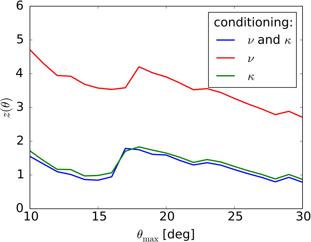 Figure 1
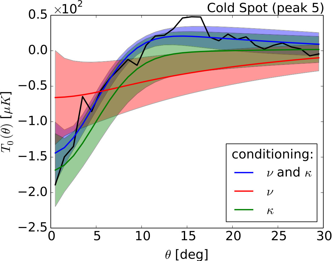 Figure 2
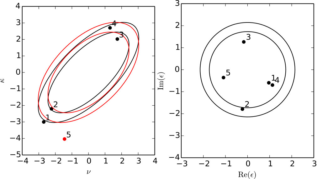 Figure 3
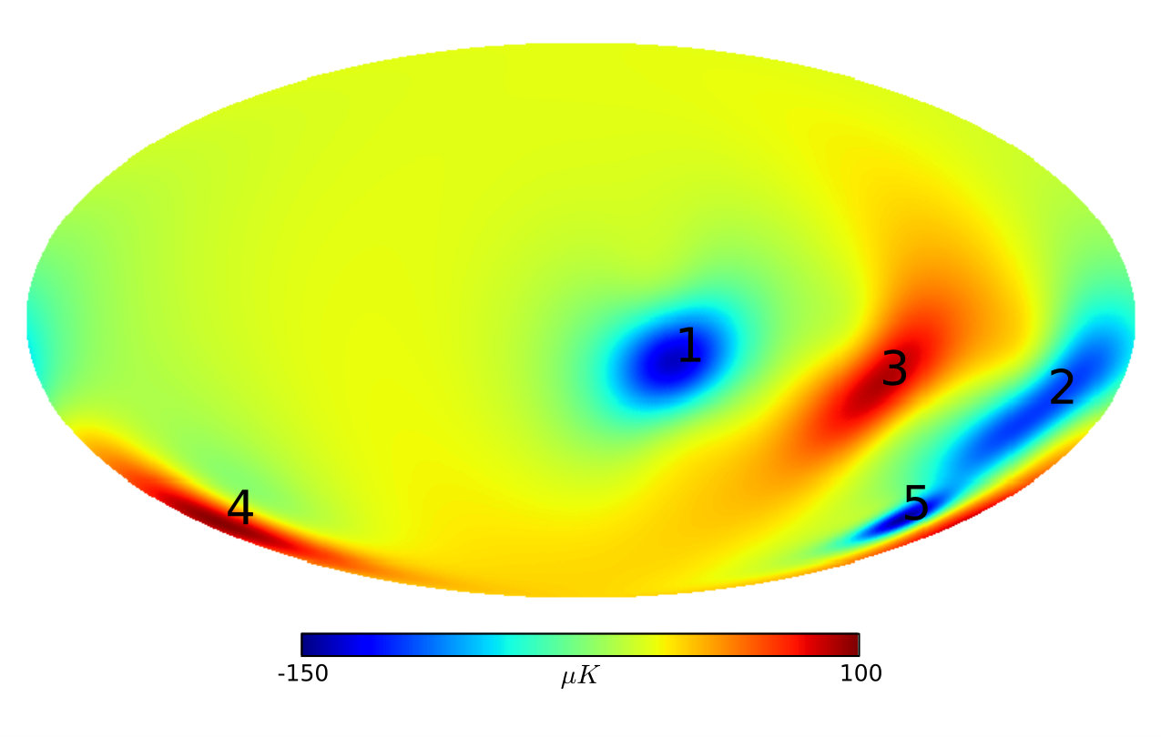 Figure 4
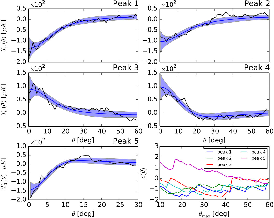 Figure 5
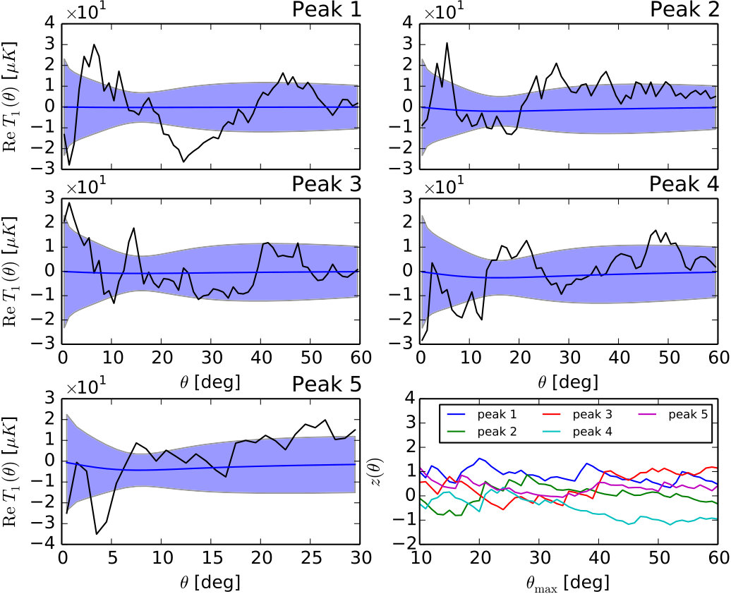 Figure 6
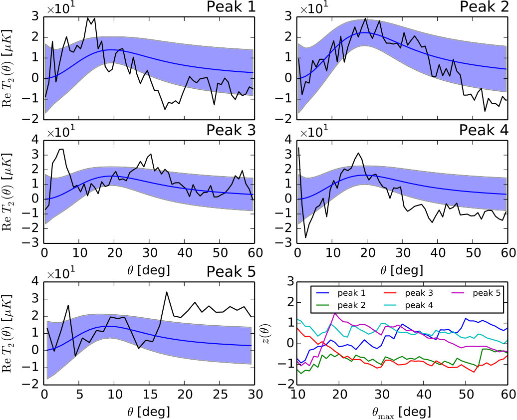 Figure 7
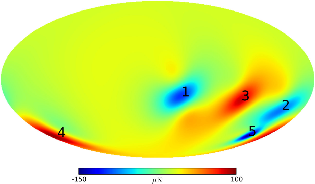 Figure 8
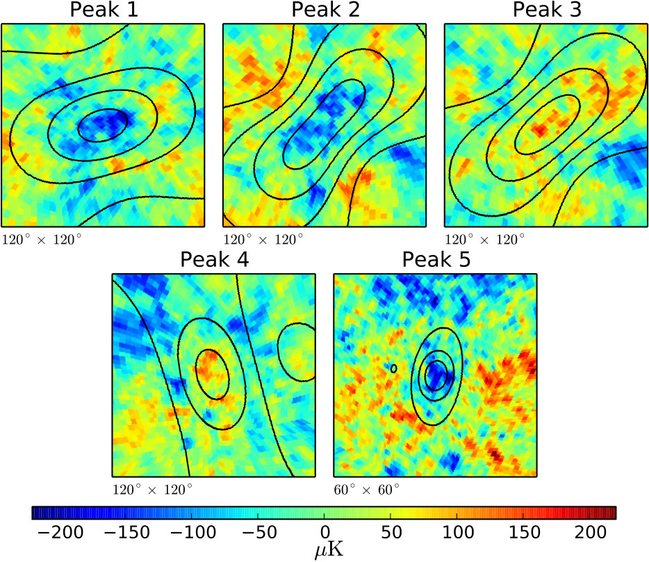 Figure 9
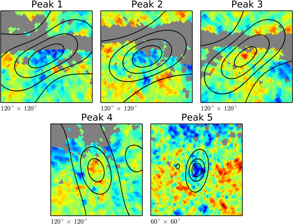 Figure 10
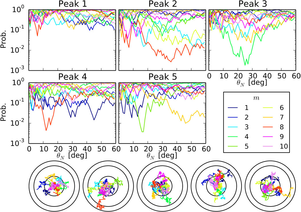 Figure 11
Peer Reviews
No public reviews on file for this paper yet. If you reviewed it on a platform where reviews are public (OpenReview, ICLR, NeurIPS, ICML), you can paste yours below so the community can read it here.
Videos
No videos yet. Explain this paper in a talk, walkthrough, or lecture? Add one.
Local properties of the large-scale peaks of the CMB temperature
A. Marcos-Caballero
E. Martínez-González
and P. Vielva
Abstract
In the present work, we study the largest structures of the CMB temperature measured by Planck in terms of the most prominent peaks on the sky, which, in particular, are located in the southern galactic hemisphere. Besides these large-scale features, the well-known Cold Spot anomaly is included in the analysis. All these peaks would contribute significantly to some of the CMB large-scale anomalies, as the parity and hemispherical asymmetries, the dipole modulation, the alignment between the quadrupole and the octopole, or in the case of the Cold Spot, to the non-Gaussianity of the field. The analysis of the peaks is performed by using their multipolar profiles, which characterize the local shape of the peaks in terms of the discrete Fourier transform of the azimuthal angle. In order to quantify the local anisotropy of the peaks, the distribution of the phases of the multipolar profiles is studied by using the Rayleigh random walk methodology. Finally, a direct analysis of the 2-dimensional field around the peaks is performed in order to take into account the effect of the galactic mask. The results of the analysis conclude that, once the peak amplitude and its first and second order derivatives at the centre are conditioned, the rest of the field is compatible with the standard model. In particular, it is observed that the Cold Spot anomaly is caused by the large value of curvature at the centre.
1 Introduction
The anisotropies in the Cosmic Microwave Background (CMB) are described inside the standard model of cosmology, which assumes that the initial perturbations are distributed according to a Gaussian in a homogeneous and isotropic Universe. The recent measurements of the CMB allow one to determine the cosmological parameters with high precision [1], showing an overall agreement between data and the concordance cosmological model. Although, in general, this agreement is large, some anomalies are found in the CMB at large scales. The characterization of these deviations have an important role in understanding the process which leads to the initial perturbations, and hence, in the characterization of the inflationary model.
Different large-scale anomalies are found in the CMB, which were first detected in the WMAP data ([2], see also references below) and confirmed later by Planck [3]. Among them, it is included the lack of correlations on large scales [4, 5] which might leads to a low variance in the temperature field [6]. In particular, in terms of the angular power spectrum, the low variance anomaly can be seen as a deficit of power in the lowest multipoles, in particular in the quadrupole and octopole [7]. Explanations in terms of an early fast-roll phase of the inflation field preceding the standard slow-roll phase have been proposed [8, 9].
On the other hand, when the temperature field is expanded in terms of the spherical harmonics, an unlikely alignment between the quadrupole and the octopole is observed [10, 11]. The interference between the two multipoles produce large-scale features in the CMB temperature aligned with the ecliptic plane, which, in particular, have more power in the southern hemisphere. The hemispherical asymmetry, which is seen in the low multipoles range (), was first detected in [12] by looking at the ratio of the power spectrum amplitude calculated on opposing hemispheres, and later extended to include smaller scales in [13]. This particular asymmetry axis is also found in the dipole modulation, which has been studied in real space [14, 15], as well as in harmonic space in order to take into account the scale dependence in the analysis [3].
Moreover, parity asymmetries have been also analysed concluding that there exists a difference in the variance of the odd and even components of the temperature field [16, 17, 18]. These studies have been extended including a directional dependence in the parity asymmetry estimator in several works [19, 20], indicating that the preferred axis for parity violations could correspond to the quadrupole and octopole alignment direction. Since the parity asymmetry measures the correlation between antipodal points on the sphere, this anomaly can be related to the lack of power at large scales [21].
In the present paper, we study the large-scale features on the CMB temperature by identifying the most prominent peaks and analysing their statistical properties. These largest peaks correspond to structures located in the galactic southern hemisphere, more precisely, in the quadrant where the south ecliptic pole is located. This region of the sky corresponds to the direction where some of the above mentioned anomalies are located (power asymmetry or dipole modulation). Besides this directional asymmetries, the interference of the quadrupole and the octopole induces an excess of power in the ecliptic southern hemisphere which is caused by their particular alignment [22]. Additionally, although it is not a peak as large as the others we consider, the Cold Spot [23, 24] is also included in the analysis since it presents an anomalous peak curvature. All these structures correspond in part to the “fingers” and spots studied in [25]. Moreover, in a recent paper [26], a multiscale analysis reveals that these peaks are the most outstanding large-scale deviations in terms of either the amplitude or the curvature.
The paper is organized as follows: in Section 2, the large-scale peaks are selected in the temperature field, characterizing their local shape through the derivatives up to second order. The analysis of the peaks is performed in terms of the radial shape of the multipolar profiles in Section 3, whereas the study of their phase correlations is considered in Section 4. In order to implement a partial sky coverage properly, the work is completed with an analysis of the peaks directly in real space. Finally, the summary and conclusions of the paper are outlined in Section 6.
2 Characterization of the large-scale peaks
The peaks in the CMB correspond to local maxima or minima in the temperature field, and they had been considered as useful geometrical descriptors of the statistical properties of the primordial radiation [27, 28, 29, 30, 31]. In order to have an extremum, constraints on the field derivatives have to be imposed. Firstly, the critical point condition implies that the gradient of the temperature must vanish at the peak location, but additionally, in order to exclude possible saddle points, it is imposed that the Hessian matrix is positive or negative definite, depending whether the extremum is a minimum or a maximum. Therefore, it is natural to characterize the peaks theoretically by conditioning the first and second derivatives at the centre of the peak, as well as the corresponding peak height. Following the notation in [31], the derivatives on the sphere are calculated by using the spin raising and lowering operators:
[TABLE]
where the derivatives are normalized in order to have dimensionless quantities with unit variance. This set of parameters corresponds to our peak degrees of freedom, which consist in two scalars ( and ), one vector () and one -spinor (). Whilst the value of the temperature at the extremum is given by the peak height , the local curvature is described by the Laplacian, which is proportional to . On the other hand, the spinorial quantities and represent the gradient and the eccentricity tensor, respectively. The components of these two spinors expressed in the helicity basis are given by complex numbers, whose real and imaginary parts describe geometrical aspects of the peak. For instance, the local eccentricity of the peak is proportional to the modulus of , whereas its phase represents the particular direction of the principal axes on the sky. Regarding the gradient, the real and imaginary parts of correspond to the components of the first derivatives in the orthogonal local system of reference. Theoretically, the gradient at the peak location must vanish by definition, but we maintain this degree of freedom as non-zero in the formalism because, in practice, there is a residual gradient due to the fact that we are selecting peaks as local extrema in a discretised field, which prevents us to impose . Although this non-null value of the first derivative is very small compared to its standard deviation, analysis based on conditioning the derivatives are very sensitive to small variations of the conditioned values. In terms of the peak shape, this effect causes a dipolar asymmetry at distances larger than the peak size (see figure 8 in Section 5).
In this work, we consider the five large-scale peaks given in figure 1. In a recent paper [26], a complete analysis of deviations on the derivatives fields is performed at different scales, concluding that these peaks are the most anomalous structures at large scales. The peaks labeled by - correspond to two maxima and two minima selected in the CMB temperature field filtered with a Gaussian with . These peaks are the most prominent large-scale structures in the sky, which are located in the same ecliptic hemisphere. The particular value of is chosen so that these large-scale fluctuations are highlighted. On the other hand, the peak labeled by is the well-known CMB anomaly called the Cold Spot [24], which is included in the analysis because is the most outstanding large-scale deviation in terms of the curvature [26], contributing to the non-Gaussianity of the temperature field [23, 24]. The Cold spot is usually characterized as a minimum in the Spherical Mexican Hat Wavelet (SMHW) [32] coefficient map at the scale . As the SMHW is obtained from the Laplacian of the Gaussian function, the coefficients map is equivalent to the curvature field of the temperature, filtered with a Gaussian with the same scale than the SMHW. Since there is a strong correlation between and at large scales, a minimum in the curvature corresponds to a minimum in the temperature field itself. For this reason, we equivalently define the Cold Spot as a minimum in at the scale .
In order to calculate the variances of the derivatives and other theoretical quantities, a particular model has to be considered. The following fiducial model is assumed: , , , , and , which represent the Planck TT-lowP best-fit cosmological parameters ([1], table 3).
The values of the derivatives at the centre of the peaks obtained from the Planck Commander map [33] are represented in figure 2. The scalar degrees of freedom and are depicted in the same plane, showing the contours of the one-point probability density function. Since the correlation between and depend on the scale where the peak is selected, it is expected that the ellipses for the peaks - () are narrower than the ones for the peak , whose scale is smaller (). On the other hand, the one-point distribution of the eccentricity tensor does not depend on the scale [31], and therefore the probability contours are the same of all the peaks. The Cold Spot (peak ) is the peak which presents a higher deviation in the - plane, mainly caused by the large value of . This value differs from the SMHW coefficient reported in [24] and confirmed by [3] for the same scale, giving a lower probability of finding a Cold Spot in the CMB temperature. The main difference between these calculations is that, whereas in this work the value of is calculated by normalizing by the theoretical variance , in [24] and [3] the value of the SMHW coefficient is calculated by using the variance estimated from the data, which is affected by the low variance of the measured CMB field at large scales [6, 3]. On the other hand, the eccentricity of the Cold Spot is within the level, which implies that its shape is almost circular [34].
The deviation of the peaks derivatives with respect to the standard model is considered by calculating the expected number of peaks with and as extreme as the corresponding observed values which are present in one realization of the temperature field (see [31] for the expression of the number density of peaks on the sphere). These numbers are for the Cold Spot and for the largest cold spot at (peak ), whereas the rest of the peaks have an expected number per realization . This implies that a peak as extreme as the Cold Spot in terms of and is expected in every realizations of the CMB temperature, given a more likely probability for the Cold Spot than the calculation in [24], which considers a larger value for the curvature at the centre of the peak, as explained above.
3 Multipolar profiles
In this section, we study the shape of the largest peaks observed in the CMB temperature. Following the formalism of [31], the shape of the peaks can be studied through the multipolar profiles, which consist in the coefficients of the Fourier transform of the azimuthal angle around the peak:
[TABLE]
where the coordinates and represent the radial and azimuthal coordinates, respectively, centered at the peak location. The monopolar profile with corresponds to the standard profile, which takes into account the spherical symmetric component of the peak. On the other hand, the higher order profiles describe different asymmetrical shapes, depending on the multipole . For instance, the profiles with and represent a dipole and a quadrupole around the peak, respectively.
The derivatives at the centre of the peak affects to the local shape depending on its spin. In particular, if the values of , , and are fixed at the centre, it is obtained the following mean profiles [31]:
[TABLE]
and for . In these equations, we have assumed that the peak is selected in the temperature field filtered with the window function , whereas the profiles are calculated from a field observed with a beam . The bias parameters characterizing the mean profiles depend on the particular values of the derivatives at the centre:
[TABLE]
where is the correlation coefficient between and . As it is mentioned before, despite the fact that we are selecting maxima and minima, the gradient at peak location does not vanish because of the discretization of the field. This particular residual affecting to the dipolar profile can be modelled as a small bias depending on the measured value of . This simple modelization of the bias is enough to correct all the systematic effect appearing in the subsequent analysis.
Additionally, when the local shape of the peak is fixed, the covariance of the multipolar profiles are given by [31]:
[TABLE]
Whilst the intrinsic part represents the covariance of the profile when the derivatives at the centre are not constrained, the term is the modification of the covariance due to the fact of conditioning the values of the derivatives. It is important to notice that the fact of conditioning the derivatives to some particular values only affects to the mean profiles, but not to the covariance. The intrinsic covariance can be calculated from the angular power spectra in the following way [31]:
[TABLE]
On the other hand, the contribution of the peak to the covariance of the multipolar profiles is different form zero for . In general, it can be written as:
[TABLE]
where the matrices are given by:
[TABLE]
and for . Since conditioning the derivatives reduces the variance of the field, these coefficients are always negative. These expressions can be generalised to consider scenarios where only the amplitude or the curvature are conditioned. In this case, we have that equals to or , depending on whether or is the conditioned variable.
As it is described in Section 2, the peaks - are selected in a map filtered with a Gaussian with a scale , whereas the Cold Spot is defined as a peak in . Therefore, the window function , which characterizes the smoothing of the field where the amplitude and its derivatives are calculated, is a Gaussian filter whose scale depends on the peak considered. On the other hand, the filter corresponds to the effective resolution of the maps over which the multipolar profiles are calculated.
In order to analyse the shape of the peaks, the values of , , and are conditioned to the measured values at the centre of the peak. The observed monopolar, dipolar and quadrupolar profiles are compared with the theoretical predictions in figures 3-5. In the case of the quadrupolar profile, a rotation is performed in order to align the principal axes with the system of reference of the peak, such that only the real part has non-zero expectation value. Statistical deviations from the standard model are quantified using a test as a function of the maximum value of considered in the analysis. Assuming that the CMB temperature is a Gaussian random field, the conditional probability of the multipolar profiles obtained fixing the values of the derivatives at the centre is also Gaussian, therefore the test is appropriate for the analysis. It is computed the following quantity for each value, which is approximately normally distributed for a large number of degrees of freedom:
[TABLE]
where represents the maximum value of considered in the test, and is the number of degrees of freedom of the variable corresponding to that value of . Whereas for the value of is equal to the number of bins considered, for any other multipole it is twice the number of bins due to the fact that the profiles take complex values. In this equation, the statistics is computed from the measured profiles and the theoretical mean profiles and covariances:
[TABLE]
where the matrix is the covariance between the different bins of the multipolar profiles, which is given by the sum of eq. (3.5) and eq. (3.6). The summations in this expression are extended over the indices for which the centre of the bins take values up to the . Regarding the theoretical estimation, the mean profiles and covariance must be also averaged in each bin in order to compare with the data. This operation is equivalent to calculate the integral of the associated Legendre functions in each interval of . In the literature [35], there exists analytical formulae which allow to calculate these integrals recursively (see appendix A). Notice that both the real and the imaginary parts of the multipolar profiles are considered in the calculation of . Commonly, the peaks are oriented along the principal axes, in which case the mean value of the imaginary parts vanishes.
Since we are interested in large-scale peaks, the galactic mask is a problem in the calculation of the profiles, specially in the ones with , where the break of the isotropy of the field is critical. Deconvolution techniques based on the Toeplitz matrix can be used in order to correct the mask effect, but in the case of aggressive masking the resulting profiles are not accurately calculated. For this reason, we use an inpainted map without missing pixels, more precisely, the CMB temperature field used in the analysis of the multipolar profiles is the Planck Commander map [33], whose galactic mask region has been filled by calculating a constrained Gaussian realization. On the other hand, in Section 5, the peaks are analysed directly in real space, where the missing pixels are not problematic, and therefore the inpainting techniques are not required.
Following the expression in eq. (3.1), the multipolar profiles are calculated by averaging the pixels in rings whose width is and are centred at the different values of . Since the size of these bins is large compared with the resolution of the Planck Commander map (FWHM ), the contribution of the instrumental noise can be ignored in our analysis. On the other hand, the filter used in the calculation of the theoretical profiles and covariance is the product of a Gaussian filter characterizing the resolution of the data and the corresponding pixel window function.
In figures 3-5, it is represented the values of for the monopolar, dipolar and quadrupolar profiles, respectively. We can see that the deviation of these profiles is less than in all the peaks considered. Moreover, the multipolar profiles with values of up to have been analysed, obtaining values which are compatible at level with what is expected in the standard model.
Particularly, in the Cold Spot analysis, it is found that the monopolar profile agrees with the standard model prediction when the values of and are conditioned. On the other hand, if only the value of is fixed to the observed value whereas is averaged out using its probability density distribution (see [31]), the Cold Spot profile presents a deviation for . This result implies that the Cold Spot anomaly is mainly caused by the extremely large value of at the centre, whereas when is conditioned, no anomaly is found in the monopolar profile. In figure 6, it is represented the monopolar profiles of the Cold Spot obtained by conditioning, the peak height , the curvature , or both. Notice that the ring-shape in the Cold spot at is only recovered when both degrees of freedom are fixed, which implies that this distinctive feature is produced by a combined effect of a large value of with a relatively small absolute value of .
4 Phase correlations of the multipolar profiles
In order to detect deviations from the standard model, the statistical properties of the phases of the spherical harmonics coefficients have been studied in several works. If the CMB temperature field is non-Gaussian or anisotropic, correlations in the phases of the ’s may exists, which causes that they are not uniformly distributed in the interval . There are different statistical tests which can be applied to study the randomness of this kind of periodic variables. For instance, the Kuiper’s test, which is a generalization of the KS test for circular data, has been used in the analysis of the phases [36]. On the other hand, in [37], the study of the Rayleigh statistics and the random walk performed by the ’s in the complex plane are applied to the CMB temperature data. All the analyses considered in these works are based on the spherical harmonics coefficients, which describe the field in a particular system of reference, and therefore their results could depend on the direction of the axis. Additionally, in a previous work [38], the genus of the largest structures on the CMB () are analysed concluding that they corresponds to the ones derived from Gaussian field with random phases. In the following, the phases of the multipolar expansion centred at different peak locations are studied in terms of the multipolar profiles.
The decomposition of the field around the peaks in terms of the profiles gives information about the contribution of each multipolar pattern to the peak shape. In particular, the phases of the multipolar profiles represent the orientation of each multipole in the local system of reference centred at the peak. Given a multipole , the phases of for different values of are not independent due to the intrinsic correlations in the field, and therefore an alignment of the multipoles is expected. In order to test whether these correlations follow the standard model or not, profiles whose bins in are independent are defined. More precisely, considering bins of the radial angle labeled by , the following profiles are calculated:
[TABLE]
where the coefficients are chosen such that have unit variance and no correlation for different values of . In practice, for each value of , the coefficients correspond to the components of the lower triangular matrix obtained from the Cholesky decomposition of the inverse covariance given in eq. (3.4). Additionally, the mean profile is subtracted to the data in eq. (4.1) in order to remove the peak degrees of freedom from the phases analysis, since otherwise the phases can be correlated because we are centred in a particular point of the field with a peak. Notice that the cumulative sum in eq. (4.1) implies that only depends on the values of the temperature with radial distance from the peak centre smaller that .
As the phases of are independent, they describe a Rayleigh random walk in the complex plane for each value of . At the time step , the position of this random walk is given by
[TABLE]
In these models of random walks, the time step corresponds to the maximum radial angle considered in the multipolar profile. Notice that, if a rotation of the system of reference around the peak is performed with an angle , the positions of the random walk transform as , as can be deduced from the transformation properties of the multipolar profiles. This is just a rotation of angle of the complex plane where the random walk moves on. Since the action of the rotation group on the steps is different for each value of , we consider a random walk for different multipolar profile separately. In previous works [37] based on the spherical harmonics coefficients, different values of contribute to the steps, which implies that the resulting random walk analysis is not invariant under rotations of the axis. On the other hand, in the scenario considered in this paper, the analysis of the random walks performed by the phases of each multipolar profile only depends on the position of the peak, and not on the orientation of the local system of reference.
The distance between the random walk position at the step and the origin of the complex plane is approximately distributed following the probability density
[TABLE]
which is valid for large values of . From this equation, it can be deduced that the variable is distributed according to the Rayleigh distribution (or equivalently, follows a with two degrees of freedom). In order to achieve better precision with this formula, the value of is calculated as follows [39]:
[TABLE]
For large values of , the variable approach to the distance travelled by the random walk . Considering this definition, the variable follows the probability in eq. (4.3) with accuracy, instead of the error achieved with the standard definition of the distance ().
The analysis is based on the fact that if the phases of the profiles are correlated, the distances travelled by the random walks will be greater than the ones expected from eq. (4.3). The paths followed by the random walks obtained from the phases of the multipolar profiles of the different peaks considered are represented in figure 7. In addition, the lower tail probability of the distance travelled by the random walk at the time step is depicted.
It is possible to see some evidences of correlation of the phases for the multipole in the peaks and , whereas in the case of the peaks and , the most correlated multipoles are and , respectively. Regarding the Cold Spot (peak ), it is important to notice that the maximum correlation is reached at , the angular distance which coincides with the position of a hot ring around the centre of the Cold Spot. On the other hand, the lack of anomalies in this analysis can be seen as evidence of the low level of residuals in the Planck Commander map at full-sky.
5 Real space analysis
In the case of having an incomplete sky, the multipolar profiles with are very sensitive to the geometry of the mask. This is not the case of the monopolar profiles (), for which the standard sky fraction correction is enough to have a good estimation of the profile. Since we are interested in large-scale structures, it is very unlikely to avoid the effect of the galactic mask in the analysis of the peaks. In this section, we consider a real space approach, analysing 2-dimensional patches around the peaks in a pixel-based formalism. This allows one to take into account the mask in a simple way, as compared with the Fourier analysis provided by the multipolar profiles.
As in the previous sections, the patches around the peaks are parametrized by the polar coordinates with the peak located at the centre of the system of reference. If the peak is described by its derivatives up to second order, the mean value of the field is given as Fourier expansion in terms of the multipolar profiles with [31]:
[TABLE]
On the other hand, the covariance of the temperature around the peak can be decomposed in terms of the intrinsic covariance of the field, and the covariance due to the effect of the peak selection [31]:
[TABLE]
where is the standard correlation function between the points and of the temperature field, which does not consider the contribution of the peak, and for (defined in eq. (3.6)) represents the contribution to the covariance due to the fact that we are conditioning to the values of the derivatives at the location of the peak.
The data used to study the peaks directly in the real space are the Planck SEVEM and SMICA temperature maps, masked with their confidence masks [33]. The analysis of the 2-dimensional patches is based on the HEALPix pixelization scheme [40] of the regions around the peaks. For the largest peaks labelled by -, the CMB data is filtered with a Gaussian of FWHM in harmonic space and mapped at the resolution corresponding to . On the other hand, the Cold Spot (peak ) is analysed at with a FWHM of . The masks for the two resolutions are calculated by smoothing the full resolution mask with the corresponding Gaussian, and masking pixels below a given threshold (in our case, ). The resulting patches consist in disc-shape regions centred at the peaks with maximum radii of for the largest peaks, and for the Cold Spot, which leads to a total number of pixels for each of the peaks. The gnomic-projected CMB data at the peaks locations are represented in figure 8. Finally, the covariance and the theoretical profiles are calculated by using eqs. (3.6) and (3.2c), where, as in the case of the multipolar profiles, the window function is given by the map resolution considered and the pixel window function.
The patches obtained from the data are compared with the theoretical models of the peaks obtained after conditioning to the values of the derivatives at the centre. The goodness of fit is evaluated by using a test as a function of the maximum value of the radius considered in the analysis. No significant deviations from the theoretical models are found in the data for any of the peaks, a result which is consistent with the analysis of the multipolar profiles in Section 3. Finally, in order to check the consistency between the real space and multipolar profile methodologies, the analysis of patches is repeated with the full-sky Commander map, finding that both analysis are compatible with the standard model.
6 Conclusions
In this work, we have studied the most prominent large-scale peaks in the CMB temperature in terms of the multipolar profiles for different values of . Since the peaks are characterized by their derivatives up to second order at the centre, we pay special attention to the monopolar and quadrupolar profiles, which have expectation values different form zero in this situation. Once the theoretical mean profiles and covariances are calculated by conditioning the derivatives to the observed values, a test is performed for each peak and value of . The analysis suggests that the theoretical monopolar and quadrupolar profiles derived from the standard model present a good agreement with the profiles obtained from the data. Moreover, a broader analysis of the multipolar profiles concludes that there is no significant deviations in the profiles with up to . These results implies that there is no anomalies in the shape of the peaks considered, at least once the values of the derivatives are conditioned.
The Cold Spot anomaly previously described in [24] is considered as a deviation in the Laplacian of the temperature field at the smoothing scale . The analysis performed by conditioning both the peak height and the curvature does not indicate any anomaly in the Cold Spot monopolar profile, but, on the other hand, if only the value of is fixed, the profile exhibits a deviation up to a radius . This result shows that the Cold Spot anomaly is mainly caused by the extremely large value of at the centre, while the field around it seems to be compatible with the Gaussian correlations in the standard model. Moreover, it is observed that the hot ring in the Cold Spot around is caused by a combination of the large value of with a comparatively small peak amplitude .
The study of the multipolar profiles is completed by analysing their phases, which take into account the orientation of the different multipolar shapes around the peaks. In general, even in the case of a statistically isotropic field, the phase of the multipolar profiles are correlated for different values of theta. For this reason, in the paper, it is introduced an estimator which associates a phase-independent profile to each multipolar profile , given a fiducial model for its covariance. This allows to define a Rayleigh random walk in terms of the phases of the profiles, which moves as the value of increases. Statistical deviations from the standard model are characterized by the total length travelled by the random walk at a given time. If the distance covered by the random walk associated to a given multipolar profile is too large (too small), it means that the corresponding multipolar profile of the peak has a correlation (anti-correlation) for different values of which is greater than the one expected in the standard model, and therefore the peak presents an alignment for that value of not compatible with an isotropic field. Some alignments are observed in few multipolar profiles of some of the large-scale peaks considered. In particular, the Cold Spot presents an alignment of the profiles which is maximum at the hot ring position ().
Finally, the peaks are directly analysed in the real space by considering -dimensional patches around them. This methodology allows to take into account a galactic mask, which cannot be done in the multipolar profile expansion due to the spurious signal introduced in that case. As in the profile analysis, the peak field is compared with the theoretical expectation when the derivatives of the peak are conditioned. In particular, the direction of the elongation of each peak is fixed according to the observed eccentricity tensor. In this case, the results are compatible with the ones obtained in the multipolar profile analysis, concluding that the effect of the mask does not change the main conclusions already found with the multipolar profiles of the large-scale peaks.
Appendix A Binning of the theoretical profiles
In order to compare with the data, the theoretical profiles have to be binned in intervals of . Since these profiles are expressed in terms of the associated Legendre functions, this operation can be done by calculating the following indefinite integrals:
[TABLE]
where the normalised associated Legendre functions are introduced in order to prevent from large numbers in the calculations. On the one hand, the integrals for are calculated from the Legendre polynomials [35]:
[TABLE]
On the other hand, in the case of , the integral can be determined recursively following the expressions in [35]:
[TABLE]
where the initial conditions are given by
[TABLE]
Finally, the averaged value of the associated Legendre function in the interval is expressed as
[TABLE]
Alternatively, these integrals can be evaluated using numerical quadrature methods, but the recursive expressions above are faster and more accurate.
Acknowledgments
Partial financial support from the Spanish Ministerio de Economía y Competitividad Projects AYA2012-39475-C02-01 and Consolider-Ingenio 2010 CSD2010-00064 is acknowledged.
The reference list from the paper itself. Each links out to its DOI / PubMed record.
- 1[1] Planck Collaboration, P. A. R. Ade, N. Aghanim, M. Arnaud, M. Ashdown, J. Aumont, C. Baccigalupi, A. J. Banday, R. B. Barreiro, J. G. Bartlett, and et al., Planck 2015 results. XIII. Cosmological parameters , A&A 594 (Sept., 2016) A 13, [ ar Xiv:1502.01589 ].
- 2[2] D. N. Spergel, L. Verde, H. V. Peiris, E. Komatsu, M. R. Nolta, C. L. Bennett, M. Halpern, G. Hinshaw, N. Jarosik, A. Kogut, M. Limon, S. S. Meyer, L. Page, G. S. Tucker, J. L. Weiland, E. Wollack, and E. L. Wright, First-Year Wilkinson Microwave Anisotropy Probe (WMAP) Observations: Determination of Cosmological Parameters , Ap JS 148 (Sept., 2003) 175–194, [ astro-ph/0302209 ].
- 3[3] Planck Collaboration, P. A. R. Ade, N. Aghanim, Y. Akrami, P. K. Aluri, M. Arnaud, M. Ashdown, J. Aumont, C. Baccigalupi, A. J. Banday, and et al., Planck 2015 results. XVI. Isotropy and statistics of the CMB , A&A 594 (Aug., 2016) A 16, [ ar Xiv:1506.07135 ].
- 4[4] C. L. Bennett, M. Halpern, G. Hinshaw, N. Jarosik, A. Kogut, M. Limon, S. S. Meyer, L. Page, D. N. Spergel, G. S. Tucker, E. Wollack, E. L. Wright, C. Barnes, M. R. Greason, R. S. Hill, E. Komatsu, M. R. Nolta, N. Odegard, H. V. Peiris, L. Verde, and J. L. Weiland, First-Year Wilkinson Microwave Anisotropy Probe (WMAP) Observations: Preliminary Maps and Basic Results , Ap JS 148 (Sept., 2003) 1–27, [ astro-ph/0302207 ].
- 5[5] C. J. Copi, D. Huterer, D. J. Schwarz, and G. D. Starkman, Lack of large-angle TT correlations persists in WMAP and Planck , MNRAS 451 (Aug., 2015) 2978–2985, [ ar Xiv:1310.3831 ].
- 6[6] C. Monteserín, R. B. Barreiro, P. Vielva, E. Martínez-González, M. P. Hobson, and A. N. Lasenby, A low cosmic microwave background variance in the Wilkinson Microwave Anisotropy Probe data , MNRAS 387 (June, 2008) 209–219, [ ar Xiv:0706.4289 ].
- 7[7] M. Cruz, P. Vielva, E. Martínez-González, and R. B. Barreiro, Anomalous variance in the WMAP data and Galactic foreground residuals , MNRAS 412 (Apr., 2011) 2383–2390, [ ar Xiv:1005.1264 ].
- 8[8] C. R. Contaldi, M. Peloso, L. Kofman, and A. Linde, Suppressing the lower multipoles in the CMB anisotropies , J. Cosmology Astropart. Phys 7 (July, 2003) 002, [ astro-ph/0303636 ].