Linear-time approximation schemes for planar minimum three-edge connected and three-vertex connected spanning subgraphs
Baigong Zheng

TL;DR
This paper introduces the first linear-time polynomial approximation schemes for finding near-optimal three-edge and three-vertex connected spanning subgraphs in undirected planar graphs, significantly improving computational efficiency.
Contribution
It provides the first polynomial-time approximation schemes with linear running time for these connectivity problems in planar graphs, a notable advancement over previous methods.
Findings
Achieved (1 + ε)-approximation in linear time for both problems.
First polynomial-time approximation schemes for these problems in planar graphs.
Demonstrated practical efficiency of the algorithms.
Abstract
We present the first polynomial-time approximation schemes, i.e., (1 + {\epsilon})-approximation algorithm for any constant {\epsilon} > 0, for the minimum three-edge connected spanning subgraph problem and the minimum three-vertex connected spanning subgraph problem in undirected planar graphs. Both the approximation schemes run in linear time.
Click any figure to enlarge with its caption.
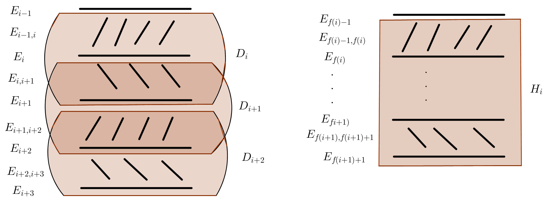 Figure 1
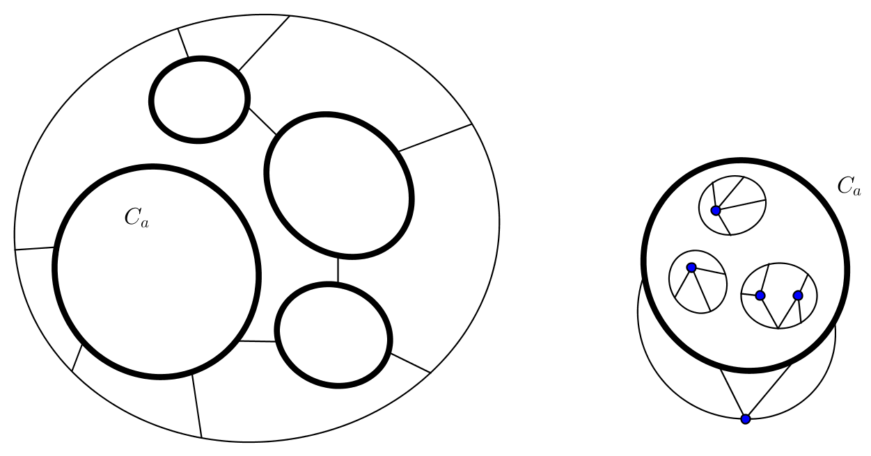 Figure 2
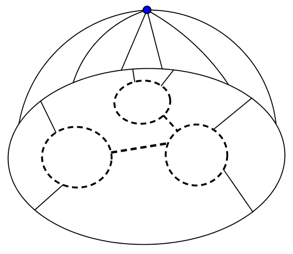 Figure 3
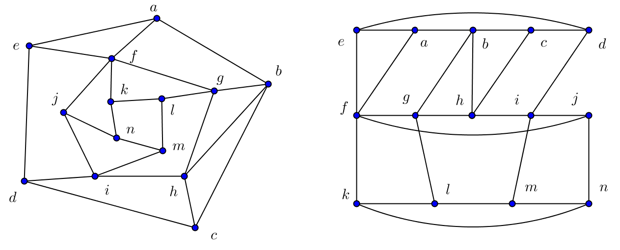 Figure 4
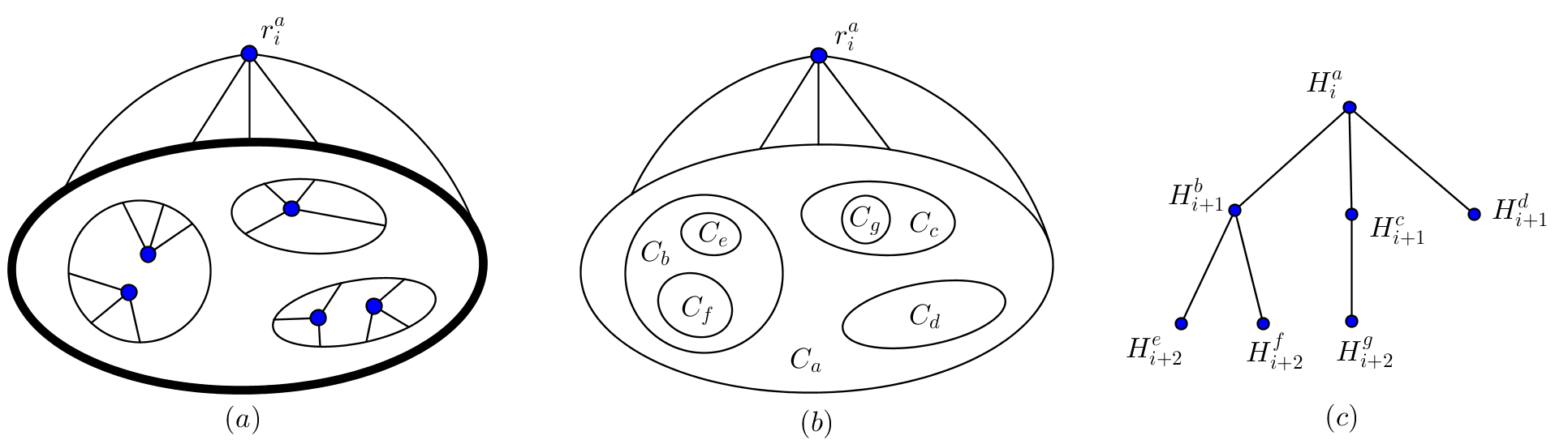 Figure 5
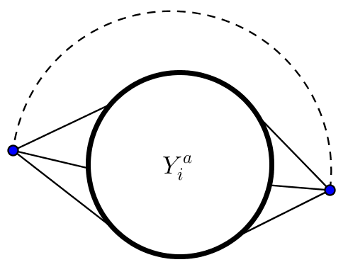 Figure 6
 Figure 7
Peer Reviews
No public reviews on file for this paper yet. If you reviewed it on a platform where reviews are public (OpenReview, ICLR, NeurIPS, ICML), you can paste yours below so the community can read it here.
Videos
No videos yet. Explain this paper in a talk, walkthrough, or lecture? Add one.
Taxonomy
TopicsComplexity and Algorithms in Graphs · Advanced Graph Theory Research · Optimization and Search Problems
Linear-time approximation schemes for planar minimum three-edge connected and three-vertex connected spanning subgraphs
Baigong Zheng
Oregon State University
Abstract
We present the first polynomial-time approximation schemes, i.e., -approximation algorithm for any constant , for the minimum three-edge connected spanning subgraph problem and the minimum three-vertex connected spanning subgraph problem in undirected planar graphs. Both the approximation schemes run in linear time.
This material is based upon work supported by the National Science Foundation under Grant No. CCF-1252833.
1 Introduction
Given an undirected unweighted graph , the minimum -edge connected spanning subgraph problem (-ECSS) asks for a spanning subgraph of that is -edge connected (remains connected after removing any edges) and has a minimum number of edges. The minimum -vertex connected spanning subgraph problem (-VCSS) asks for a -vertex connected (remains connected after removing any vertices) spanning subgraph of with minimum number of edges. These are fundamental problems in network design and have been well studied. When , the solution is simply a spanning tree for both problems. For , the two problems both become NP-hard [12, 7], so people put much effort into achieving polynomial-time approximation algorithms. Cheriyan and Thurimella [7] give algorithms with approximation ratios of for -VCSS and for -ECSS for simple graphs. Gabow and Gallagher [11] improve the approximation ratio for -ECSS to for simple graphs when , and they give a -approximation algorithm for -ECSS in multigraphs. Some researchers have studied these two problems for the small connectivities , especially and , and obtained better approximations. The best approximation ratio for -ECSS in general graphs is of Jothi, Raghavachari, and Varadarajan [17], while for -VCSS in general graphs, the best ratio is of Gubbala and Raghavachari [14]. Gubbala and Raghavachari [15] also give a -approximation algorithm for 3-ECSS in general graphs.
A polynomial-time approximation scheme (PTAS) is an algorithm that, given an instance and a positive number , finds a -approximation for the problem and runs in polynomial time for fixed . Neither -ECSS nor -VCSS have a PTAS even in graphs of bounded degree for unless P = NP [10]. However, this hardness of approximation does not hold for special classes of graphs and small values of . For example, Czumaj et al. [8] show that there are PTASes for both of 2-ECSS and 2-VCSS in planar graphs. Both problems are NP-hard in planar graphs (by a reduction from Hamiltonian cycle). Later, Berger and Grigni improved the PTAS for -ECSS to run in linear time [3].
Following their PTASes for 2-ECSS and 2-VCSS, Czumaj et al. [8] ask the following: can we extend the PTAS for -ECSS to a PTAS for 3-ECSS in planar graphs? A PTAS for 3-VCSS in planar graphs is additionally listed as an open problem in the Handbook of Approximation Algorithms and Metaheuristics (Section 51.8.1) [13]. In this paper we answer these questions affirmatively by giving the first PTASes for both 3-ECSS and 3-VCSS in planar graphs. Our main results are the following theorems.
Theorem 1**.**
For 3-ECSS, there is an algorithm that, for any and any undirected planar graph , finds a -approximate solution in linear time.
Theorem 2**.**
For 3-VCSS, there is an algorithm that, for any and any undirected planar graph , finds a -approximate solution in linear time.
In the following, we assume there are no self-loops in the input graph for both of 3-ECSS and 3-VCSS. For -ECSS, we allow parallel edges in , but at most parallel edges between any pair of vertices are useful in a minimal solution. For -VCSS, parallel edges are unnecessary, so we assume the input graph is simple. Since three-vertex connectivity (triconnectivity) and three-edge connectivity can be verified in linear time [24, 21], we assume the input graph contains a feasible solution. W.l.o.g. we also assume .
1.1 The approach
Our PTASes follow the general framework for planar PTASes that grew out of the PTAS for TSP [18], and has been applied to obtain PTASes for other problems in planar graphs, including minimum-weight 2-edge-connected subgraph [3], Steiner tree [4, 6], Steiner forest [2] and relaxed minimum-weight subset two-edge connected subgraph [5]. The framework consists of the following four steps.
Spanner Step.
Find a subgraph that contains a -approximation and whose total weight is bounded by a constant times of the weight of an optimal solution. Such a graph is usually called a spanner since it often approximates the distance between vertices.
Slicing Step.
Find a set of subgraphs, called slices, in such that any two of them are face disjoint and share only a set of edges with small weight and each of the subgraphs has bounded branchwidth.
Dynamic-Programming Step.
Find the optimal solution in each slice using dynamic programming. Since the branchwidth of each subgraph is bounded, the dynamic programming runs in polynomial time.
Combining Step.
Combine the solutions of all subgraphs obtained by dynamic programming and some shared edges from Slicing step to give the final approximate solution.
For most applications of the PTAS framework, the challenging step is to illustrate the existence of a spanner subgraph. However, for 3-ECSS and 3-VCSS, we could simply obtain a spanner from the input graph by deleting additional parallel edges since by planarity there are at most edges in and the size of an optimal solution is at least , where . So, different from those previous applications, the real challenge for our problems is to illustrate the slicing step and the combining step. For the slicing step, we want to identify a set of slices that have two properties: (1) three-edge-connectivity for 3-ECSS or triconnectivity for 3-VCSS, and (2) bounded branchwidth. With these two properties, we can solve 3-ECSS or 3-VCSS on each slice efficiently. For the combining step, we need to show that we can obtain a nearly optimal solution from the optimal solutions of all slices found in slicing step and the shared edges of slices, that means the solution should satisfy the connectivity requirement and its size is at most times of the size of an optimal solution for the original input graph.
To identify slices, we generalize a decomposition used by Baker [1]. Before sketching our method, we briefly mention the difficulty in applying previous techniques. The PTAS for TSP [18] identifies slices in a spanner by doing a breadth-first search in its planar dual to decompose the edge set into some levels, and any two adjacent slices could only share all edges of the same level, which form a set of edge-disjoint simple cycles. This is enough to achieve simple connectivity or biconnectivity between vertices of different slices. But our problems need stronger connectivity for which one cycle is not enough. For example, we may need a non-trivial subgraph outside of slice to maintain the triconnectivity between two vertices in slice . See Figure 1 (a).
For 3-ECSS, we construct a graph called 3EC slice. We contract each component of the spanner that is not in the current 3EC slice. Since contraction can only increase edge-connectivity, this will give us the 3EC slices that are three-edge connected (Lemma 14 in Section 3). However, if we directly apply this contraction method in the slicing step of the PTAS for TSP, the branchwidth of the 3EC slice may not be bounded. This is because there may be many edges that are not in the slice but have both endpoints in the slice, and such edges may divide the faces of the slice into distinct regions, each of which may contain a contracted node. See Figure 1 (b). To avoid this problem, we apply the contractions in the decomposition used by Baker [1], which define a slice based on the levels of vertices instead of edges. We can prove that each 3EC slice has bounded branchwidth in this decomposition (Lemma 12 in Section 2).
Although each 3EC slice is three-edge connected, the union of their feasible solutions may not be three-edge connected. Consider the following situation. In a solution for a slice, a contracted node is contained in all vertex-cuts for a pair of vertices and . But in , the subgraph induced by the vertex set corresponding to may not be connected. Therefore, and may not satisfy the connectivity requirement in . See Figure 1 (c).
In their paper, Czumaj et al. [8] proposed a structure called bicycle. A bicycle consists of two nested cycles, and all in-between faces visible from one of the two cycles. This can be used to maintain the three-edge-connectivity between those connecting endpoints in cycles. This motivates our idea: we want to combine this structure with Baker’s shifting technique so that two adjacent slices shared a subgraph similar to a bicycle. In this way, we could maintain the strong connectivity between adjacent slices by including all edges in this shared subgraph, whose size could be bounded by the shifting technique. Specifically, we define a structure called double layer for each level based on our decomposition, which intuitively contains all the edges incident to vertices of level and all edges between vertices of level . Then we define a 3EC slice based on a maximal circuit such that any pair of 3EC slices can only share edges in the double layer between them. In this way, we can obtain a feasible solution for 3-ECSS by combining the optimal solutions for all the slices and all the shared double layers (Lemma 16 in Section 3). By applying shifting technique on double layers, we can prove that the total size of the shared double layers is a small fraction of the size of an optimal solution. So we could add those shared double layers into our solution without increasing its size by much, and this gives us a nearly optimal solution.
For 3-VCSS, we construct a 3VC slice based on a simple cycle instead of a circuit. The construction is similar to that of 3EC slices. However, contraction does not maintain vertex connectivity. So we need to prove each 3VC slice is triconnected (Lemma 20 in Section 4). Then similar to 3-ECSS, we also need to prove that the union of the optimal solutions of all 3VC slices and all shared double layers form a feasible solution (Lemma 22 in Section 4).
For dynamic-programming step, we need to solve a minimum-weight 3-ECSS problem in each 3EC slice and a minimum-weight 3-VCSS problem in each 3VC slice. This is because we need to carefully assign weights to edges in a slice so that we can bound the size of our solution. We provide a dynamic program for the minimum-weight 3-ECSS problem in graphs of bounded branchwidth in Section 5, which is similar to that in the works of Czumaj and Lingas [9, 10]. A dynamic program for minimum-weight 3-VCSS can be obtained in a similar way. Then we have the following theorem.
Theorem 3**.**
Minimum-weight 3-ECSS problem and minimum-weight 3-VCSS problem both can be solved on a graph of bounded branchwidth in time.
2 Preliminaries
Let be an undirected planar graph with vertex set and edge set . We denote by the subgraph of induced by where is a vertex subset or an edge subset. We simplify to . We assume we are given an embedding of in the plane. We denote by the subgraph induced by the edges on the outer boundary of in this embedding. A circuit is a closed walk that may contain repeated vertices but not repeated edges. A simple cycle is a circuit that contains no repetition of vertices, other than the repetition of the starting and ending vertex. A simple cycle bounds a finite region in the plane that is a topological disk. We say a simple cycle encloses a vertex, an edge or a subgraph if the vertex, edge or subgraph is embedded in the topological disk bounded by the cycle. We say a circuit encloses a vertex, edge or subgraph if the vertex, edge or subgraph is enclosed by a simple cycle in the circuit.
The level of a vertex of is defined as follows [1]: a vertex has level [math] if it is on the infinite face of ; a vertex has level if it is on the infinite face after deleting all the vertices of levels less than . Let be the set of vertices of level . Let be the edge set of in which each edge has both endpoints in level . Let be the edge set of where each edge has one endpoint in level and one endpoint in level . See Figure 2 as an example. Then we have the following observations.
Observation 1**.**
For any level , the boundary of any non-trivial two-edge connected component in is a maximal circuit in .
Observation 2**.**
For any level , the boundary of any non-trivial biconnected component in is a simple cycle in .
For any , we define the th double layer
[TABLE]
as the set of edges in . See Figure 3
Let be a constant that depends on . For , let . Let and . Since , we have the following upper bound for the size of .
[TABLE]
Let for integer . If for any , we let . Let be the subgraph of induced by vertices in level and be a subgraph of . See Figure 3. Note that contains exactly the edges of double layers through . Therefore, so long as , we have , and for any and . So for any we have
[TABLE]
For each and each maximal circuit in , we construct a graph , called a 3EC slice, from as follows. (See Figure 4.)
Let be the subset of vertices of that are enclosed by . We contract each connected component of into a node. After all the contractions, we delete self-loops and additional parallel edges if there are more than three parallel edges between any pair of vertices. The resulting graph is the 3EC slice . We call these contracted vertices nodes to distinguish them from the original vertices of . We call a contracted node inner if it is obtained by contracting a component that is enclosed by ; otherwise it is outer. Note that a 3EC slice is still planar, and two 3EC slices only share edges in a double layer: the common edges of two 3EC slices and must be in the set , while the common edges of and must be in the set . In the similar way, we can construct a simple graph , called 3VC slice, for each and each simple cycle in .
- Remark
There can be a 3EC slice containing only two vertices in . Then the slice must contain at least two parallel edges between the two vertices in . But any 3EC slice cannot contain only one vertex in since we define 3EC slice based on a maximal circuit and we assume there is no self-loop in . Similarly, any 3VC slice contains at least three vertices in .
Lemma 4**.**
If is two-edge connected (biconnected), then each 3EC (3VC) slice obtained from has at most one outer node.
Proof.
We first prove the following claims, and then by these claims we prove the lemma.
Claim 5**.**
For any , subgraph is connected.
Proof.
We prove by induction on that subgraph is connected for any . The base case is . Since is the set of vertices on the boundary of , and since is connected, subgraph is connected. Assume subgraph is connected for . Then we claim subgraph is connected. This is because for each connected component of , there exists at least one edge between and , otherwise graph cannot be connected. Since subgraph is connected, we have is connected. ∎
Claim 6**.**
If is two-edge connected, then for any two distinct maximal circuits and in , there is a path between and that is vertex disjoint from .
Proof.
Note that and are vertex-disjoint, otherwise is not maximal. We argue that there cannot be two edge-disjoint paths between and in . If there are such two edge-disjoint paths, say and , then cannot be a maximal circuit in : if and have the same endpoint in , then is not maximal; otherwise there is some edge of that cannot be in . So we know that any vertex in and any vertex in cannot be two-edge connected in . Since is two-edge connected and since must be outside of and , vertices in and those in must be connected through . Therefore, there exists a path from to that does not contain any vertex in . ∎
Similarly, we can obtain the following claim.
Claim 7**.**
If is biconnected, then for any two distinct simple cycles and in , there is a path between and that is vertex disjoint from .
Now we prove the lemma. Let be a 3EC slice based on some maximal circuit in for some . Let be the set of all vertices of that have levels less than , and be a two-edge connected component in disjoint from . Then the boundary of is a maximal circuit in . Note that could be trivial and then is also trivial. Since is connected, each simple cycle must enclose a connected subgraph of . So circuit must enclose a connected subgraph of . By Claim 6, there is a path between and disjoint from . Since is connected by Claim 5, the set of vertices that are not enclosed by induces a connected subgraph of , giving the lemma for . For 3VC slice, we can obtain the lemma in the same way by Claim 5 and Claim 7. ∎
Using this lemma, we show how to construct all the 3EC slices in linear time. First we compute the levels of all vertices in linear time by using an appropriate representation of the planar embedding such as that used by Lipton and Tarjan [20]. We construct all 3EC slices from in time. We first contract all the edges between vertices of level . Next, we identify all two-edge connected components in , which can be done in linear time by finding all the edge cuts by the result of Tarjan [26]. Each such component contains a maximal circuit in . Based on these two-edge connected components of , we could identify for all 3EC slices in time, where is the outer contracted node for . This is because the inner contracted nodes of a 3EC slice is the same as those contracted in if they are enclosed by . Then for each 3EC slice we add the outer node , and for each vertex we add an edge between and if there is an edge between and some vertex that is not enclosed by . To add those edges, we only need to travel all the edges of subgraph . Since all these steps run in time, and since , we can obtain the following lemma.
Lemma 8**.**
All 3EC slices can be constructed in time.
Since we can compute all the biconnected components in in linear time based on depth-first search by the result of Hopcroft and Tarjan [16], we can obtain a similar lemma for 3VC sllices in a similar way.
Lemma 9**.**
All 3VC slices can be constructed in time.
We review the definition of branchwidth given by Seymour and Thomas [25]. A branch decomposition of a graph is a hierarchical clustering of its edge set. We represent this hierarchy by a binary tree, called the decomposition tree, where the leaves are in bijection with the edges of the original graph. If we delete an edge of this decomposition tree, the edge set of the original graph is partitioned into two parts and according to the leaves of the two subtrees. The set of vertices in common between the two subgraphs induced by and is called the separator corresponding to in the decomposition. The width of the decomposition is the maximum size of the separator in that decomposition, and the branchwidth of is the minimum width of any branch decomposition of . We borrow the following lemmas from Klein and Mozes [19], which are helpful in bounding the branchwidth of our graphs.
Lemma 10**.**
(Lemma 14.5.1 [19])* Deleting or contracting edges does not increase the branchwidth of a graph.*
Lemma 11**.**
(Lemma 14.6.1 [19] rewritten)* There is a linear-time algorithm that, given a planar embedded graph , returns a branch-decomposition whose width is at most twice of the depth of a rooted spanning tree of .*
Lemma 12**.**
If is two-edge connected (biconnected), the branchwidth of any 3EC (3VC) slice is .
Proof.
We prove this lemma for 3EC slices when is two-edge connected; by the same proof we can obtain the lemma for 3VC slices when is biconnected. Let be a 3EC slice. By Lemma 4, there is at most one outer contracted node for . Let the level of be , and the level of all inner contracted nodes be . Now we add edges to ensure that every vertex of level has a neighbor of level for each , while maintaining planarity. Call the resulting graph . Then the branchwidth of is no more than that of by Lemma 10. Now we can find a breadth-first-tree of rooted at that has depth at most . By Lemma 11, the branchwidth of is and that of is at most . ∎
3 PTAS for -ECSS
In this section, we prove Theorem 1. W.l.o.g. we assume has at most three parallel edges between any pair of vertices. Then is our spanner. Let be an optimal solution for . Since each vertex in has degree at least three, we have
[TABLE]
If is simple, then by planarity the number of edges is at most three times of the number of vertices. Since there are at most three parallel edges between any pair of vertices, we have
[TABLE]
Combining (3) and (4), we have .
In this section, we only consider 3EC slices. So when we say slice, we mean 3EC slice in this section. We construct all the slices from . By (1), we have the following
[TABLE]
We borrow the following lemma from Nagamochi and Ibaraki [22].
Lemma 13**.**
(Lemma 4.1 (2) [22] rewritten)* Let be a -edge connected graph with more than 2 vertices. Then after contracting any edge in , the resulting graph is still -edge connected.*
Recall that our slices are obtained from by contractions and deletions of self-loops. By the above lemma, we have the following lemma.
Lemma 14**.**
If is three-edge connected, then any slice is three-edge connected.
Since we can include all the edges in shared double layers, they are “free” to us. So we would like to include those edges as many as possible in the solution for each slice. This can be achieved by defining an edge-weight function for each slice : assign weight [math] to edges in and weight to other edges. By Lemma 14, any slice is three-edge connected. We solve the minimum-weight 3-ECSS problem on in linear time by Theorem 3. Let be a feasible solution for the minimum-weight 3-ECSS problem on . Then it is also a feasible solution for 3-ECSS on . Let be an optimal solution for the minimum-weight 3-ECSS problem on . Then we have the following observation.
Observation 3**.**
The weight of any solution is the same as the number of its common edges with , that is
[TABLE]
Let be the set of all maximal circuits in . Then we have the following lemmas.
Lemma 15**.**
For any , let . Then we can bound the number of edges in by the following inequality
[TABLE]
Proof.
We show that is a feasible solution for the minimum-weight 3-ECSS problem on , and then we bound the size of . Let be the set of vertices of that are not contracted nodes. We first contract connected components of just as constructing from . Then we need to identify any two contracted nodes, if their corresponding components in are in the same connected component in . See Figure 5.
Finally, we delete all the self-loops and extra parallel edges if there are more than three parallel edges between any two vertices. The resulting graph is a subgraph of and spans . Since identifying two nodes maintains edge-connectivity, and since contractions also maintain edge-connectivity by Lemma 13, the resulting graph is three-edge connected. So is a feasible solution for minimum-weighted 3-ECSS problem on . Then by the optimality of , we have . And by Observation 3, we have
[TABLE]
Note that for any slice , we have and . Since for distinct (vertex-disjoint) maximal circuits and in , subgraphs and are vertex-disjoint, we have the following equalities.
[TABLE]
[TABLE]
Then
[TABLE]
So we have . ∎
Lemma 16**.**
The union is a feasible solution for .
Proof.
For any and any maximal circuit , let be the graph obtained from by uncontracting all its inner contracted nodes. See Figure 6. By Lemma 4, there is at most one outer node for each slice .
Define a tree based on all the slices: each slice is a node of , and two nodes and are adjacent if they share any edge and . Root at the slice , which contains the boundary of . Let be the subtree of that roots at slice . See Figure 6 as an example. For each child of , let be the boundary of . Then is the maximal circuit in that is shared by and . Further, by the construction of , graph is a subgraph of .
We prove the lemma by induction on this tree from leaves to root. Assume for each child of , there is a feasible solution for the graph such that . We prove that there is a feasible solution for such that . For the root of , we have , and then the lemma follows from the case .
The base case is that is a leaf of . When is a leaf, there is no inner contracted node in and we have . So is a feasible solution for .
Recall that and only share edges of and vertices of . Let be any inner contracted node of and be the vertex set of the connected component of corresponding to . We need the following claim.
Claim 17**.**
If for some , then is connected.
Proof.
By the construction of levels, all the vertices on the boundary of have level . See Figure 7. Then all the edges of are in . So subgraph is connected. Let be any vertex in and let be any vertex in that has level . Then is not in . Since is a feasible solution for , there exists a path from to in . This path must intersect by planarity. So and any vertex on the boundary of are connected in , giving the claim. ∎
Let and be any two vertices of . To prove the feasibility of , we prove and are three-edge connected in . Let and . Then . Depending on the locations of and , we have three cases.
Case 1: .
Note that we could construct in the following way. Initially we have . For any inner contracted node of , let be the vertex set of its corresponding connected component in . Then there exists a child of such that , and we replace with in . We do this for all inner contracted nodes of . Finally we add some edges of into the resulting graph such that . Then the resulting is the same as by the definition of . We prove that any pair of the remaining vertices in are three-edge connected during the construction. This includes the remaining inner contracted nodes of during the process, but after all the replacements, there is no such inner contracted nodes, proving the case.
By the definition of , any pair of vertices of are three-edge connected in . Assume after the first replacements, any pair of the remaining vertices in are three-edge connected in the resulting graph . Let be the next inner contracted node to be replaced, be the vertex set of its corresponding component and be the resulting graph after replacing . Let be the child of such that . Let be the simple cycle in that encloses . Then all vertices of have level and are shared by and . Further, . Let and be any two remaining vertices of . There are three edge-disjoint -to- paths and three edge-disjoint -to- paths in , all of which must intersect . So there exist three edge-disjoint -to- paths and three edge-disjoint -to- paths in . Now we delete two edges in . If these two edges are not both in , then the vertices of are still connected. Then one remaining -to- path and one remaining -to- path together with the rest of witness the connectivity between and . If the two deleted edges are both in , then there exist one -to- path and one -to- path after the deletion. By Claim 17, subgraph is connected. So all vertices of are connected in . Then and are connected after the deletion. Finally, after replacing all the inner contracted nodes, we only add edges of into , which will not break three-edge-connectivity between any pair of vertices. This finishes the proof of Case 1.
Case 2: .
Let be the graph contains and be the graph contains . (The two graphs could be identical.) Let (resp. ) be the simple cycle in (resp. ) that enclose (resp. ). (The two cycles and could be identical.) Since is three-edge connected, there are three edge-disjoint paths from to some vertex of in . All these three paths must intersect , so there are three edge-disjoint paths from to in . Similarly, there are three edge-disjoint paths from to in . Now we delete any two edges in . After the deletion, there exist one -to- path and one -to- path where and . Since all vertices in have level and are in , they are three-edge connected in by Case 1. This means there exists a path from to after the deletion. Therefore, and are connected after deleting any two edges in , giving the three-edge-connectivity.
Case 3: and .
Let be the graph containing . Then there is a vertex in . By Case 1, vertices and are three-edge connected, and by Case 2, vertices and are three-edge connected. Then vertices and are three-edge connected by the transitivity of three-edge-connectivity.
This completes the proof of Lemma 16. ∎
Proof of Theorem 1.
We first prove correctness of our algorithm, and then prove its running time. By Lemma 16, is a feasible solution. Thus
[TABLE]
Let , and then we obtain .
Let be the number of vertices of graph . We could find and construct all slices in time by Lemma 8. By Lemma 12, each slice has branchwidth . So by Theorem 3, we could solve the minimum-weight 3-ECSS on each slice in linear time for fixed . Based on those optimal solutions for all slices, we could construct our solution in time. Therefore, our algorithm runs in time. ∎
4 PTAS for -VCSS
In this section, we prove Theorem 2. W.l.o.g. assume is simple. Then is our spanner. Let be an optimal solution for . Since is simple and planar, we have . Then by (3) we have . In this section, we only consider 3VC slices. So in the following, we simplify 3VC slice to slice. We first construct slices from . By (1), we have the following
[TABLE]
Similar to 3-ECSS, we want to solve a minimum-weight 3-VCSS problem on each slice. But before defining the weights for this problem on each slice, we first need to show any slice is triconnected. The following lemma is proved by Vo [27], we provide a proof for completeness.
Lemma 18**.**
([27])* Let be a simple cycle of that separates into two parts: and . Let be any connected component of . If is triconnected, then , the graph obtained from by contracting , is triconnected.*
Proof.
Let be the contracted node of . Then and any other vertex of are triconnected since is triconnected. Let and be any two vertices of distinct from . To prove the lemma, we show and are triconnected. Since and are triconnected, there are three vertex-disjoint paths between and . Note that all the three paths must intersect cycle since form a cut for and all the other vertices in . Similarly, there are three vertex-disjoint paths between and , all of which intersect cycle . Now we delete any two vertices different from and in . If the two deleted vertices are both in , then there exist one -to- path and one -to- path after the deletion, which witness the connectivity between and . If the two deleted vertices are not both in , the remaining vertices in are connected and then the remaining -to- path and the remaining -to- path together with the rest of edges in witness the connectivity between and . So and are triconnected. ∎
By the same proof, we can obtain the following lemma.
Lemma 19**.**
Let be a simple cycle of . Let and be two vertices of whose neighbors in are all in . Then if is triconnected, the graph obtained from by identifying and is triconnected.
Let be the set of all simple cycles in . Then we have the following lemma.
Lemma 20**.**
For any and any simple cycle , the slice is triconnected.
Proof.
Let be the set of vertices of that are not contracted nodes. We could obtain by contracting each connected component of into a node. Each time we contract a connected component of , there is a simple cycle that separates and other vertices: if is outside of , then ; otherwise is some simple cycle in that encloses . Then by Lemma 18 the resulting graph is still triconnected after each contraction. Therefore, the final resulting graph is triconnected. ∎
Now we define the edge-weight function on a slice : we assign weight 0 to edges in and weight 1 to other edges. Then we solve the minimum-weight 3-VCSS problem on slice by Theorem 3. Let be a feasible solution for the minimum-weight 3-VCSS problem on . Then it is also a feasible solution for 3-ECSS on . Let be an optimal solution for this problem on . Then we can prove the following two lemmas, whose proofs follow the same outlines of the proofs of Lemmas 15 and 16 respectively.
Lemma 21**.**
For any , let . Then we can bound the number of edges in by the following inequality
[TABLE]
Proof.
We first show is a feasible solution for minimum-weighted 3-VCSS problem on any slice . Let be the set of vertices of that are not contracted nodes. We first contract each component of into a node. The resulting graph after each contraction is still triconnected by Lemma 18. After all the contractions, we identify any two contracted nodes and if their corresponding components in are connected in . This implies there exists a simple cycle in or such that all neighbors of and are in . So by Lemma 19 the resulting graph after each identification is also triconnected. Finally we delete parallel edges and self-loops if possible. After identifying all possible nodes, the resulting graph has the same vertex set as and is triconnected. Since the resulting graph is a subgraph of , we know is a feasible solution for minimum-weighted 3-VCSS problem on .
Note that for any slice , we have . By the optimality of , we have . Since all the nonzero-weighted edges are in , Observation 3 still holds. Then we have
[TABLE]
Since for distinct (edge-disjoint) simple cycles and in , subgraphs and are vertex-disjoint, we have the following equalities.
[TABLE]
[TABLE]
Then
[TABLE]
So we have . ∎
Lemma 22**.**
The union is a feasible solution for .
Proof.
For any and any simple cycle , let be the graph obtained from slice by uncontracting all the inner contracted nodes of . By Lemma 4, there is at most one outer contracted node for any slice .
Define a tree based on all the slices: each slice is a node of , and two nodes and are adjacent if they share any edge and . Root at the slice , which contains the boundary of . Let be the subtree of that roots at slice . For each child of , let be the simple cycle in that is shared by and . Then is the boundary of .
We prove the lemma by induction on this tree from leaves to root. Assume for each child of , there is a feasible solution for the graph such that . We prove that there is a feasible solution for such that . For the root of , we have , and then the lemma follows from the case .
The base case is that is a leaf of . When is a leaf, there is no inner contracted node in and we have . So is a feasible solution for .
We first need a claim the same as Claim 17. Note that any inner contracted node of is enclosed by some cycle . Let be any inner contracted node of that is enclosed by , and be the vertex set of the connected component of corresponding to . Then we have the following claim, whose proof is the same as that of Claim 17.
Claim 23**.**
If for some , then is connected.
Now we ready to prove is a feasible solution for . That is, we prove it is triconnected. Let and be any two vertices of . Let . Since , we have four cases.
Case 1: .
For any contracted component in that corresponds to an inner contracted node of , by Claim 23 all vertices in are connected in if . Then all vertices of are connected in , since for any child of we have . By the triconnectivity of , there are three vertex-disjoint paths between and in . Since each inner contracted node of could be in only one path witnessing connectivity, the three vertex-disjoint -to- paths in could be transferred into another three vertex-disjoint -to- paths in by replacing each contracted inner contracted node with a path in the corresponding component . So and are triconnected in .
Case 2: .
Since is a cut for vertices enclosed by and those not enclosed by , by the triconnectivity of we have . By inductive hypothesis, is a feasible solution for , so there are three vertex-disjoint -to- paths in . All these three paths must intersect by planarity, so there are three vertex-disjoint -to- paths in . Similarly, there are three vertex-disjoint -to- paths in . If we delete any two vertices in , then there exist at least one -to- path and one -to- path for some vertices . Since all vertices in have level , they are in . Then by Case 1, vertices and are triconnected in , so they are connected after deleting any two vertices. Therefore, and are also connected after the deletion.
Case 3: and .
If one of and is in , they are triconnected by Case 1 or 2. So w.l.o.g. we assume is not enclosed by and is strictly enclosed by . Since is triconnected, we have . We could delete any two vertices in and there exists at least one vertex in . By Case 1, vertices and are connected after the deletion, and by Case 2, vertices and are connected after the deletion. So and are connected after the deletion.
Case 4: and .
W.l.o.g. assume is strictly enclosed by and is strictly enclosed by , otherwise, by Case 3 they are triconnected. Since is triconnected, we have . After deleting any two vertices in , there exists a vertex . By Case 2, vertices and are connected after deletion, and by Case 3 vertices and are connected after deletion. So and are connected after deletion.
This completes the proof of Lemma 22. ∎
Proof of Theorem 2.
We first prove the correctness, and then prove the running time. Let the union be our solution. By Lemma 22, the solution is feasible for . Then we have
[TABLE]
We set and then we have .
Let be the number of vertices in graph . We could find the edge set in linear time. By Lemma 9 we could construct all slices in time. So the slicing step runs in linear time. By Lemma 12, the branchwidth of each slice is . Therefore, we could solve the minimum-weight 3-VCSS problem on each slice in linear time by Theorem 3. Based on the optimal solutions for all the slices, we could construct our final solution in linear time. So our algorithm runs in linear time. ∎
5 Dynamic Programming for Minimum-Weight -ECSS on graphs with bounded branchwidth
In this section, we give a dynamic program to compute the optimal solution of minimum-weighted -ECSS problem on a graph with bounded branchwidth . This will prove Theorem 3 for the minimum-weight 3-ECSS problem. Our algorithm is inspired by the work of Czumaj and Lingas [9, 10]. Note that need not be planar.
Given a branch decomposition of , we root its decomposition tree at an arbitrary leaf. For any edge in , let be the separator corresponding to it, and be the subset of mapped to the leaves in the subtree of that does not include the root of . Let be a spanning subgraph of . We adapt some definitions of Czumaj and Lingas [9, 10]. An separator completion of is a multiset of edges between vertices of , each of which may appear up to times.
Definition 1**.**
A configuration of a vertex of for an edge of is a pair , where is a tuple , representing that there are edge-disjoint paths from to the th vertex of in , and is a set of tuples , representing that there are edge-disjoint paths between the vertices and of in . (We only need those configurations where for all and for all .) All the paths in a configuration should be mutually edge-disjoint in .
Definition 2**.**
For any pair of vertices and in , let be the set of separator completions of each of which augments to a graph where and are three-edge connected. For each vertex in , let be a set of configurations of for . Let be the set of all the non-empty in which all tuples can be satisfied in . Let be the set consisting of one value in each for all pairs of vertices and in , and be the set consisting of one value in each for all vertices in . We call the tuple the connectivity characteristic of , and denote it by .
Note that for any edge . Subgraph may correspond to multiple and , so may have multiple connectivity characteristics. Further, each value in represents at least one vertex. For any edge , there are at most distinct separator completions ( pairs of vertices, each of which can be connected by at most parallel edges) and at most distinct sets of separator completions. For any edge , there are at most different configurations for any vertex in since the number of different sets is at most , the number of different sets is at most (the same as the number of separator completions). So there are at most different sets of configurations , and at most different sets . Therefore, there are at most distinct connectivity characteristics for any edge .
Definition 3**.**
A configuration of vertex for is connecting if the inequality holds where is the th coordinate in . That is, there are enough edge-disjoint paths from to the corresponding separator which can connect and vertices outside . is connecting if all configurations in its set are connecting. Subgraph is connecting if at least one of is connecting. In the following, we only consider connecting subgraphs and their connecting connectivity characteristics.
In the following, we need as a subroutine an algorithm to solve the following problem: when given a set of demands and a multigraph, we want to decide if there exist edge-disjoint paths between vertices and in the graph and all the paths are mutually edge-disjoint. Although we do not have a polynomial time algorithm for this problem, we only need to solve this on graphs with vertices, edges and demands. So even an exponential time algorithm is acceptable for our purpose here. Let be an algorithm for this problem, whose running time is bounded by a function , which may be exponential in .
For an edge in the decomposition tree , let and be its two child edges. Let () be a spanning subgraph of (). Let . Then we have the following lemma.
Lemma 24**.**
For any pair of and , all the possible , that could be obtained from and , can be computed in time.
Proof.
We compute all the possible sets for the three components of .
Compute all possible Each contains two parts: the first part covers all pairs of vertices in the same for and the second part covers all pairs of vertices from distinct subgraphs.
For the first part, we generalize each value for into a possible set . Notice that each separator completion can be represented by a set of demands where and are in the separator. For a candidate separator completion of , we combine with each to construct a graph and define the demand set the same as . By running on this instance, we can check if is a legal generalization for . This could be computed in time for each . All the legal generalizations for form .
Now we compute the second part. Let and be the configurations for some pair of vertices and respectively. We will compute possible . We first construct a graph on by the two configurations: add parallel edges between two vertices if there are paths between them represented in the configurations. Then we check for each candidate separator completion if and are three-edge connected in . We need for this checking if we use Orlin’s max-flow algorithm [23]. All those that are capable of providing three-edge-connectivity with form . This can be computed in time for each pair of configurations.
A possible consists of each value in for every for and each value in for all pairs of configurations of and . To compute all the sets, we need at most time. There are at most sets and each may contain at most values. Therefore, to generate all the possible from those sets, we need at most time.
Compute all possible We generalize each configuration of in () into a set of possible configurations. For each set in , we construct a graph by , and on vertex set : if there are disjoint paths between a pair of vertices represented in , or , we add parallel edges between the same pair of vertices in , taking time. For a candidate value for , we define a set of demands according to and and run on all the possible we construct for sets in . If there exists one such graph that satisfies all the demands, then we add this candidate value into . We can therefore compute each set in time. A possible consists of each value in for all . There are at most such sets and each may contain at most values. So we can generate all possible from those sets in time.
Compute For each pair of and , we construct a graph on vertex set : if two vertices are connected by disjoint paths, we add parallel edges between those vertices in . Since each candidate for can be represented by a set of demands, we only need to run on all possible to check if can be satisfied. We add all satisfied candidates into . This can be computed in time.
Therefore, the total running time is . For each component we enumerate all possible cases, and the correctness follows. ∎
Our dynamic programming is guided by the decomposition tree from leaves to root. For each edge , our dynamic programming table is indexed by all the possible connectivity characteristics. Each entry indexed by the connectivity characteristic in the table is the weight of the minimum-weight spanning subgraph of that has as its connectivity characteristic.
Base case
For each leaf edge of , the only subgraph is the edge and the separator only contains the endpoints and . contains the multisets of edge that appears twice. contains two configurations: and , and contains two configurations: and . contains one set: .
For each non-leaf edge in , we combine every pair of connectivity characteristics from its two child edges to fill in the dynamic programming table for . The root can be seen as a base case, and we can combine it with the computed results. The final result will be the entry indexed by in the table of the root. Let . Then the size of the decomposition tree is . By Lemma 24, we need time to combine each pair of connectivity characteristics. Since there are at most connectivity characteristics for each node, the total running time will be . Since the branchwidth of is bounded, the running time will be .
Correctness
The separator completions guarantee the connectivity for the vertices in , and the connecting configurations enumerate all the possible ways to connect vertices in and vertices of . So the connectivity requirement is satisfied. The correctness of the procedure follows from Lemma 24.
Acknowledgements
We thank Glencora Borradaile and Hung Le for helpful discussions.
The reference list from the paper itself. Each links out to its DOI / PubMed record.
- 1[1] B. Baker. Approximation algorithms for NP-complete problems on planar graphs. Journal of the ACM , 41(1):153–180, 1994.
- 2[2] M. Bateni, M. Hajiaghayi, and D. Marx. Approximation schemes for Steiner forest on planar graphs and graphs of bounded treewidth. J. ACM , 58(5):21, 2011.
- 3[3] A. Berger and M. Grigni. Minimum weight 2-edge-connected spanning subgraphs in planar graphs. In Proceedings of the 34th International Colloquium on Automata, Languages and Programming , volume 4596 of Lecture Notes in Computer Science , pages 90–101, 2007.
- 4[4] G. Borradaile, C. Kenyon-Mathieu, and P. Klein. A polynomial-time approximation scheme for Steiner tree in planar graphs. In Proceedings of the 18th Annual ACM-SIAM Symposium on Discrete Algorithms , volume 7, pages 1285–1294, 2007.
- 5[5] G. Borradaile and P. Klein. The two-edge connectivity survivable network problem in planar graphs. In Proceedings of the 35th International Colloquium on Automata, Languages and Programming , pages 485–501, 2008.
- 6[6] G. Borradaile, P. Klein, and C. Mathieu. An O ( n log n ) 𝑂 𝑛 𝑛 {O}(n\log n) approximation scheme for Steiner tree in planar graphs. ACM Transactions on Algorithms , 5(3):1–31, 2009.
- 7[7] J. Cheriyan and R. Thurimella. Approximating minimum-size k-connected spanning subgraphs via matching. SIAM Journal on Computing , 30(2):528–560, 2000.
- 8[8] A. Czumaj, M. Grigni, P. Sissokho, and H. Zhao. Approximation schemes for minimum 2-edge-connected and biconnected subgraphs in planar graphs. In Proceedings of the fifteenth Annual ACM-SIAM Symposium on Discrete Algorithms , pages 496–505. Society for Industrial and Applied Mathematics, 2004.