Kneser ranks of random graphs and minimum difference representations
Zolt\'an F\"uredi, Ida Kantor

TL;DR
This paper investigates the Kneser rank and minimum difference representations of random graphs, establishing bounds proportional to n/ log n for these parameters with high probability.
Contribution
It provides probabilistic bounds for the Kneser rank and minimum difference representations of random graphs, extending previous results and applying to various graph representations.
Findings
Kneser rank of random graphs is proportional to n/ log n
Bounds for minimum difference representations are established for bipartite graphs
Results hold with high probability as n grows large
Abstract
Every graph is an induced subgraph of some Kneser graph of rank , i.e., there is an assignment of (distinct) -sets to the vertices such that and are disjoint if and only if . The smallest such is called the Kneser rank of and denoted by . As an application of a result of Frieze and Reed concerning the clique cover number of random graphs we show that for constant there exist constants , such that with high probability \[ c_1 n/(\log n)< f_{\rm Kneser}(G) < c_2 n/(\log n). \] We apply this for other graph representations defined by Boros, Gurvich and Meshulam. A {\em -min-difference representation} of a graph is an assignment of a set to each vertex such that \[ ij\in E(G) \,\, \Leftrightarrow \, \, \min \{|A_i\setminus A_j|,|A_j\setminus A_i|…
Click any figure to enlarge with its caption.
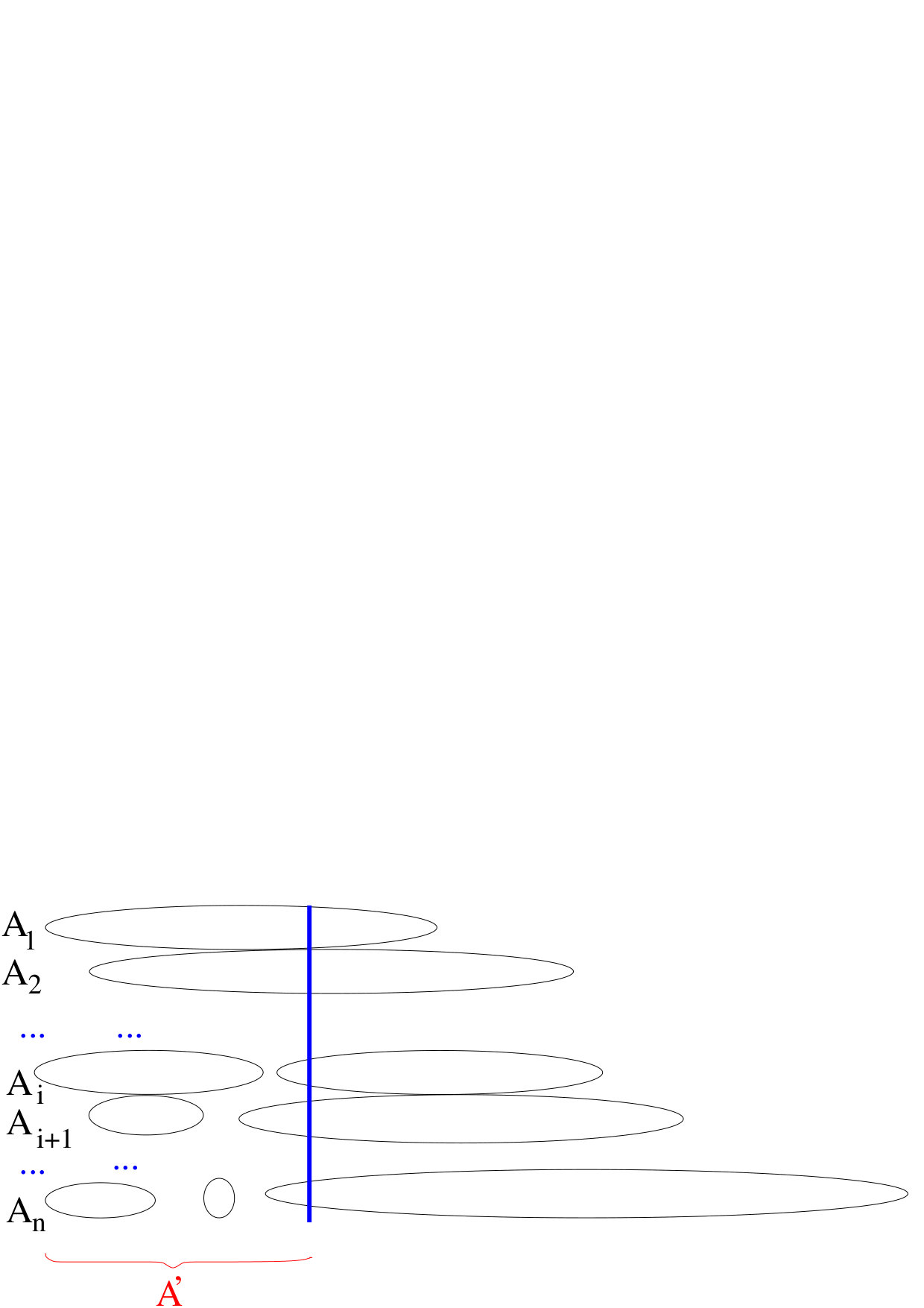 Figure 1
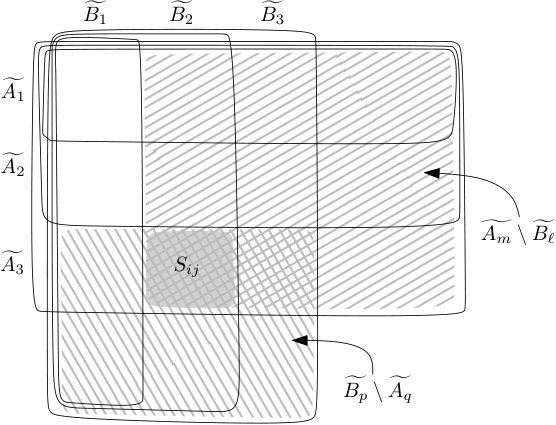 Figure 2
Peer Reviews
No public reviews on file for this paper yet. If you reviewed it on a platform where reviews are public (OpenReview, ICLR, NeurIPS, ICML), you can paste yours below so the community can read it here.
Videos
No videos yet. Explain this paper in a talk, walkthrough, or lecture? Add one.
Taxonomy
TopicsLimits and Structures in Graph Theory · Advanced Graph Theory Research · Finite Group Theory Research
00footnotetext: Keywords and Phrases: random graphs, Kneser graphs, clique covers, intersection graphs.
2010 Mathematics Subject Classification: 05C62, 05C80. [Furedi_Kantor_final.tex]
Submitted to ??? Printed on
Kneser ranks of random graphs and minimum difference representations
Zoltán Füredi1 and Ida Kantor2 **Research was supported in part by grant (no. K116769) from the National Research, Development and Innovation Office – NKFIH, by the Simons Foundation Collaboration Grant #317487, and by the European Research Council Advanced Investigators Grant 267195.**Supported by project 16-01602Y of the Czech Science Foundation (GACR).
( 1 Alfréd Rényi Institute of Mathematics, Budapest, Hungary
(e-mail: [email protected])
2 Charles University, Prague
(e-mail: [email protected]) )
Abstract
Every graph is an induced subgraph of some Kneser graph of rank , i.e., there is an assignment of (distinct) -sets to the vertices such that and are disjoint if and only if . The smallest such is called the Kneser rank of and denoted by . As an application of a result of Frieze and Reed concerning the clique cover number of random graphs we show that for constant there exist constants , such that with high probability
[TABLE]
We apply this for other graph representations defined by Boros, Gurvich and Meshulam.
A -min-difference representation of a graph is an assignment of a set to each vertex such that
[TABLE]
The smallest such that there exists a -min-difference representation of is denoted by . Balogh and Prince proved in 2009 that for every there is a graph with . We prove that there are constants such that holds for almost all bipartite graphs on vertices.
1 Kneser representations
A representation of a graph is an assignment of mathematical objects of a given kind (intervals, disks in the plane, finite sets, vectors, etc.) to the vertices of in such a way that two vertices are adjacent if and only if the corresponding sets satisfy a certain condition (intervals intersect, vectors have different entries in each coordinate, etc.). Representations of various kinds have been studied extensively, see, e.g., [7], [10], the monograph [15], or from information theory point of view [13]. The representations considered in this paper are assignments to the vertices of a graph such that the ’s are (finite) sets satisfying certain relations.
The Kneser graph (for positive integers ) is a graph whose vertices are all the -subsets of the set , and whose edges connect two sets if they are disjoint. An assignment for a graph (where ) is called a Kneser representation of rank if each has size , the sets are distinct, and and are disjoint if and only if .
Every graph on vertices with minimum degree has a Kneser representation of rank . To see that, define the co-star representation of . For every , let be the set of the edges adjacent to in the complement of (this is the graph with and ). We have if , otherwise , and the maximum size of is . To turn the co-star representation into a Kneser representation add pairwise disjoint sets of labels to the sets to increase their cardinality to exactly . The resulting sets are all distinct, they have the same intersection properties as , and form a Kneser representation of of rank .
Let denote the set of (labelled) graphs on and let denote the family of graphs on having a Kneser representation of rank . is equivalent to the fact that is an induced subgraph of some Kneser graph . We have
[TABLE]
Let denote the smallest such that has a Kneser representation of rank . We have seen that . We show that there are better bounds for almost all graphs.
Theorem 1**.**
There exist constants such that for with high probability
[TABLE]
We will prove a stronger version as Corollary 12.
2 Minimum difference representations
In difference representations, generally speaking, vertices are adjacent if the representing sets are sufficiently different. As an example consider Kneser graphs, where the vertices are adjacent if and only if the representing sets are disjoint. There are other type of representations where one joins sets close to each other, e.g., -intersection representations were investigated by M. Chung and West [6] for dense graphs and Eaton and Rödl [7] for sparse graphs. But these are usually lead to different type of problems, one cannot simply consider the complement of the graph.
This paper is mostly focused on -min-difference representations (and its relatives), defined by Boros, Gurvich and Meshulam in [5] as follows.
Definition 2**.**
Let be a graph on the vertices . A -min-difference representation of is an assignment of a set to each vertex so that
[TABLE]
Let be the set of graphs with that have a -min-difference representation. The smallest such that is denoted by .
The co-star representation (which was investigated by Erdős, Goodman, and Pósa [8] in their classical work on clique decompositions) shows that exists and it is at most .
Boros, Collado, Gurvits, and Kelmans [4] showed that many -vertex graphs, including all trees, cycles, and line graphs, the complements of the above, and -free graphs, belong to . They did not find any graph with . Boros, Gurvitch and Meshulam [5] asked whether the value of over all graphs is bounded by a constant. This question was answered in the negative by Balogh and Prince [3], who proved that for every there is an such that whenever , then for a graph on vertices we have with high probability. Their proof used a highly non-trivial Ramsey-type result due to Balogh and Bollobás [2], so their bound on is a tower function of .
Our main result is a significant improvement of the Balogh-Prince result. Let denote the family of bipartite graphs with partite sets and , .
Theorem 3**.**
There is a constant such that for almost all bipartite graphs one has .
Let be a graph on vertices with . One of the basic facts about random graphs is that almost all graphs on vertices contain as an induced subgraph. The following theorem is an easy consequence of this fact together with Theorem 3.
Corollary 4**.**
There is a constant such that almost all graphs on vertices satisfy
[TABLE]
3 On the number of graphs with –min-dif representations
3.1 The structure of min-dif representations of bipartite graphs
Analogously to previous notation, (and ) denotes the family of (bipartite) graphs with labelled vertices (partite sets and , , respectively) with . Our aim in this Section is to show that there exists a constant such that if . This implies that for almost all bipartite graphs on vertices .
A -min-difference representation of is reduced if deleting any element from all sets that contain it yields a representation of a graph different from . Note that
[TABLE]
so the graph corresponding to the -representation has no more edges than , . There is a natural partition of the elements of : for every , we have the subset ( where is the complement of the set . We call these subsets atoms. If a -min-difference representation is reduced, then no atom has more than elements. It follows that the ground set of a reduced representation of an -vertex graph has no more than elements. Lemma 5 improves on this observation.
Lemma 5**.**
Let be a graph with vertices and a reduced -min-difference representation of . Then
[TABLE]
Proof.
Define the sets in the cases and . Let . The number of elements in is bounded above by the quantity . We claim that . Otherwise, if there is an element , then the representation can be reduced, defines the same graph as .
The upper bound in Lemma 5 can be significantly improved for bipartite graphs.
Lemma 6**.**
Let be a bipartite graph with labeled vertices, . Let and be the sets representing the two parts. If is a reduced -min-difference representation of , then
[TABLE]
Proof.
Suppose that and . Let and , . Define
[TABLE]
For each , the inequality follows from the assumption that . The vertices in each part of form an independent set, so for each , we have . Hence .
If for some , then there is an index such that and therefore . In other words, if and then . Therefore the sets form a chain (see Figure 1),
[TABLE]
Treat the other part of analogously: define and note the same bound on its size, and note that the sets form a chain.
Let us define . We will prove that there are at most sets of the form and , each of cardinality , covering . Therefore contains at most elements. For each , let us define and . Let and . The sets form a chain, same for . The elements of belong to atoms (as defined in the beginning of this section), many of them possibly empty, corresponding to the squares in Figure 2.
For each , , , the atom is defined as . Since the representation is reduced, no elements from the atom can be left out, so e.g., . It follows that either there are some and such that and the atom belongs in (here and ), or there are some such that and the atom is in . Since , we have in the first case. Likewise in the second case, . In Figure 2, the first option corresponds to a rectangle containing the cell and the upper-right corner, with all the squares in this rectangle together containing only at most elements. The second option corresponds to a similar rectangle with only at most elements in it, containing the square and the lower-left corner.
Call a subrectangle critical if , and similarly is critical if . Our argument above can be reformulated that every (nonempty) cell is covered by a critical rectangle. This implies that in each row one can find at most two critical rectangles that cover all non-empty atoms in it. This yields the desired upper bound .
Finally, altogether .
3.2 Counting reduced matrices
Let be a set of size . In this subsection we give an upper bound for the number of sequences of subsets of satisfying the following two properties
(P1) ,
(P2) (for all ).
Let be the [math]- matrix that has the characteristic vectors of the sets as its rows (in this order). The positions in where an entry 1 is directly above an entry 0 will be called one-zero configurations, while the positions where a 0 is directly above a 1 will be called zero-one configurations. A column in a 0-1 matrix is uniquely determined by the locations of the one-zero configurations and the zero-one configurations unless it is a full 0 or full 1 column. We count the number of possible matrices by filling up the entries in three steps.
Each one-zero configuration corresponds to an and to an element . A set can be selected in at most
[TABLE]
ways (). Do this for each , altogether we have less than ways to write in the one-zero configurations into .
Select in each column the top . If there is no such element in a column we indicate that it is blank, a full zero column. There are at most outcomes for each column, altogether there are at most possibilities. Fill up with [math]’s each column above its top . Define as in (1), . We have . The columns of that correspond to the elements of have a (possibly empty) string of zeros followed by a string of ones. We almost filled up and we can finish this process by selecting the remaining zero-one configurations.
There may be several zero-one configurations in a single column. Each of them has a unique (closest, or smallest indexed) above them. That element is already written in into our still partially filled , because that element 1 (even if it is the top element) belongs to a unique one-zero configuration. This correspondence is an injection. So there are at most zero-one configurations in the columns corresponding to which are not yet identified. There are at most ways to select them.
Since (for )
[TABLE]
we obtain the following
Claim 7**.**
Altogether, there are ways to fill with entries in according to the rules (P1) and (P2).
3.3 Proofs of the lower bounds
Proof of the lower bound in Theorem 3..
Let be a bipartite graph with both parts of size and suppose that belongs to . By Lemma 6 we may suppose that has a reduced -min-difference representation such that each representing set is a subset of , where . There are permutations and which rearrange the sets according their sizes and . Consider the matrices, , whose ’th row is the [math]- characteristic vector of and , respectively. The permutations , and the matrices , completely describe . The matrices satisfies properties (P1) and (P2), so Claim 7 yields the following upper bound for the number of such fourtuples
[TABLE]
Here the right hand side is if implying that for almost all the bipartite graphs.
Proof of the lower bound for the random bipartite graph..
Recall that in a random graph , each of the edges occurs independently with probability . Similarly, denotes the class of graphs with the probability of a given graph is
[TABLE]
Here the right hand side is at most . This implies that for any class of graphs the probability is at most times this upper bound. If the class of graphs is too small, namely
[TABLE]
then for one has
[TABLE]
Taking with a sufficiently small , we obtain
Corollary 8**.**
For constant there exists a constant such that the following holds for with high probability as
[TABLE]
4 Maximum and average difference representations
Boros, Gurvich and Meshulam [5] also defined -max-difference representations and -average-difference representations of a graph in a natural way, that is, the vertices and are adjacent if and only if for the corresponding sets , we have and , respectively. Analogously to we can define and . Since for every graph a Kneser representation is a min-dif, average-difference, and max-difference representation as well we get
[TABLE]
Let , , (, ) denote the family of graphs and in with labeled vertices or with partite sets and , , respectively, such that (, respectively).
It was proved in [5] that and are not bounded by a constant, for a matching of size one has and . (It turns out that .) The proof of Theorem 3 can be easily adapted for these parameters for as well. Even more, we can handle the general case , too.
Corollary 9**.**
For constant there exists a constant such that the following holds for with high probability as
[TABLE]
Similarly for with high probability we have
[TABLE]
These lower bounds together with the upper bounds from Corollary 14 below imply that for almost all vertex graphs, and for almost all bipartite graphs on vertices, and are .
Sketch of the proof..
If (and if ) and is a -max-difference (-average-difference) representation then
[TABLE]
holds for each pair . If the representation is reduced, then we obtain (without the tricky proof of Lemma 6) that , and the same holds for , too. The conditions of Claim 7 are satisfied implying
[TABLE]
We complete the proof of (5) applying (3) as it was done at the end of the previous Section.
Consider a graph and let be a reduced -max-difference representation. (The case of -average-difference representation can be handled in the same way, and the details are left to the reader). The only additional observation we need is that since (7) holds for each non-edge , we have for all pairs of vertices whenever . Thus for every reduced representation (in case of ) one has . Also, for . Then the conditions of Claim 7 are fulfilled (with instead of ) implying the following version of (2)
[TABLE]
where denotes the class of graphs with .
We complete the proof of (6) by applying (3) and the fact that
[TABLE]
holds with high probability for .
5 Clique covers of the edge sets of graphs
We need the following version of Chernoff’s inequality (see, e.g., [1]). Let be mutually independent random variables with and all . Let . Then
[TABLE]
A finite linear space is a pair consisting of a set of elements (called points) and a set of subsets of (called lines) satisfying the following two properties.
Any two distinct points belong to exactly one line .
Any line has at least two points.
In other words, the edge set of the complete graph has a clique decomposition into the complete graphs , .
Lemma 10**.**
For every positive integer there exists a linear space with lines such that , every edge has size , and every point belongs to lines.
Proof.
(Folklore). If where is a power of a prime then we can take the lines of an affine geometry . Each line has exactly points and each point belongs to lines. In general, one can consider the smallest power of prime with (we have ) and take a random -set and the lines defined as , .
5.1 Thickness of clique covers
The clique cover number of a graph is the minimum number of cliques required to cover the edges of graph . Frieze and Reed [9] proved that for constant, , there exist constants , such that for with high probability
[TABLE]
They note that ‘a simple use of a martingale tail inequality shows that is close to its mean with very high probability’. We only need the following consequence concerning the expected value.
[TABLE]
The thickness of a clique cover of is the maximum degree of the hypergraph , i.e., . The minimum thickness among the clique covers of is denoted by .
A clique cover corresponds to a set representation in a natural way with the property that and are disjoint if and only if is a non-edge of . The size of the largest is the thickness of . For one can add distinct extra elements to (for each ), thus obtaining a Kneser representation of rank of the complement of , . This relation can be reversed, yielding
[TABLE]
Theorem 11**.**
For constant there exist constants , such that for with high probability
[TABLE]
Proof.
The lower bound is easy. The maximum degree of with high probability satisfies . As usual we write as tends to infinity. Also for the unproved but well-known statements concerning the random graphs see the monograph [12]. The size of the largest clique with high probability satisfies . Since we may choose .
The upper bound probably can be proved by analyzing and redoing the clever proof of Frieze and Reed concerning . Probably their randomized algorithm yields the upper bound for the thickness, too. Although there are steps in their proof where they remove from (as cliques of size 2) an edge set of size and one needs to show that these edges are well-distributed. However, one can easily deduce the upper bound for directly only from Equation (9).
Given , fix a linear hypergraph with point set and hyperedges provided by Lemma 10. We have , , and every point belongs to lines. Build the random graph in steps by taking a . Let be a clique cover of with members, .
Let denote the thickness of at the point . We consider as a random variable, whose distribution is depending only on and . For every , we have
[TABLE]
Here with very high probability satisfies . Then (9) implies that
[TABLE]
Since the distributions of and are identical (for ), and there are terms on the left hand side, we obtain that
[TABLE]
Here we chose .
Let be the thickness of at . We have , where this is a sum of mutually independent random variables, and each term is non-negative and is bounded by . Define independent random variables
[TABLE]
for each with . We can apply Chernoff’s inequality (8) for any real
[TABLE]
Substituting the right hand side is and we get
[TABLE]
Since this is true for all , we obtain that (for large enough ) for any
[TABLE]
completing the proof of the upper bound for .
Since the complement of a random graph is a random graph from , Theorem 11 and (10) imply that
Corollary 12**.**
For constant , there exist constants , such that for with high probability
[TABLE]
One can also prove a similar upper bound for the random bipartite graph.
Corollary 13**.**
For constant there exist a constant such that for with high probability
[TABLE]
Proof.
Let a random bipartite graph with partite sets . Consider a random graph and , their union is . We can consider as a member of . Since can be obtained from by adding two complete graphs and , we obtain
[TABLE]
where the last inequality holds with high probability according to Theorem 11.
Recall (4), that for every graph , holds. These and the above two Corollaries imply the following upper bounds.
Corollary 14**.**
For constant the following holds for with high probability as
[TABLE]
and similarly for
[TABLE]
6 Prague dimension
The Prague dimension (it is also called product dimension) of a graph is the smallest integer such that one can find vertex distinguishing good colorings . This means that for every edge and but for every non-edge , there exists an with , moreover the vectors and are distict for . Two vertices are adjacent if and only if their labels disagree in every . As Hamburger, Por, and Walsh [11] observed, the Kneser rank never exceeds the Prague dimension, so one can extend (4) as follows. For every graph
[TABLE]
The determination of is usually a notoriously difficult task. The results of Lovász, Nešetřil, and Pultr [14] were among the first (non-trivial) applications of the algebraic method. Hamburger, Por, and Walsh [11] observed that there are graphs where the difference of is arbitrarily large, even for Kneser graphs . Poljak, Pultr, and Rödl [16] proved that (as is fixed and ) while for all . Still we think that for most graphs these parameters have the same order of magnitude.
Conjecture 15**.**
For a constant probability there exists a constant , such that for with high probability
[TABLE]
A matching lower bound (with high probability) follows from (11) and Corollary 12. We think the same order of magnitude holds for the case when is bipartite.
Conjecture 16**.**
For a constant probability there exists a constant , such that for with high probability
[TABLE]
6.1 Prague dimension and clique coverings of graphs
The chromatic index of a clique cover of the graph is the chromatic index of the hypergraph , i.e., is the smallest that one can decompose the clique cover into parts, such that the members of each are pairwise (vertex)disjoint. The minimum chromatic index among the clique covers of is denoted by . In other words, can be covered by subgraphs with complete graph components. Obviously, the thickness is a lower bound . Here the left hand side is at most for almost all graphs by Theorem 11. We think that the Frieze–Reed [9] method can be applied to find the correct order of magnitude of , too.
Conjecture 17**.**
For constant, , there exists a constants such that for with high probability
[TABLE]
One can observe that (similarly as and are related, see (10)) there is a remarkable simple connection between Prague dimension and .
[TABLE]
So Conjectures 15 and 17 are in fact equivalent, and Conjecture 17 also implies Conjecture 16.
7 Conclusion
We have considered five graph functions , , , , and , which are hereditary (monotone for induced subgraphs) and two random graph models and . We gave an upper bound for the order of magnitude for eight of the possible ten problems, and we have also have conjectures for the missing two upper bounds (Conjectures 15 and 16). We also established matching lower bounds in seven cases, which also gave probably the best lower bound in two more cases (concerning ). All of these 19 estimates were . In the last case (in Corollary 4) we have a weaker bound, so it is natural to ask that
Problem 18**.**
Is it true that for any fixed for with high probability one has ?
Let us remark that if is a complement of a triangle-free graph then the Kneser rank and Prague dimension is or . So it can be . For example, . No such results are known for .
Problem 19**.**
What is the maximum of over the set of -vertex graphs ? Is it true that for every and ?
The reference list from the paper itself. Each links out to its DOI / PubMed record.
- 1[1] N. Alon and J. H. Spencer , The probabilistic method , Wiley Series in Discrete Mathematics and Optimization, John Wiley & Sons, Inc., Hoboken, NJ, fourth ed., 2016.
- 2[2] J. Balogh and B. Bollobás , Unavoidable traces of set systems , Combinatorica, 25 (2005), pp. 633–643.
- 3[3] J. Balogh and N. Prince , Minimum difference representations of graphs , Graphs Combin., 25 (2009), pp. 647–655.
- 4[4] E. Boros, R. Collado, V. Gurvich, and A. Kelmans , On 2-representable graphs , manuscript, DIMACS REU Report, July, (2000).
- 5[5] E. Boros, V. Gurvich, and R. Meshulam , Difference graphs , Discrete Math., 276 (2004), pp. 59–64. 6th International Conference on Graph Theory.
- 6[6] M. S. Chung and D. B. West , The p 𝑝 p -intersection number of a complete bipartite graph and orthogonal double coverings of a clique , Combinatorica, 14 (1994), pp. 453–461.
- 7[7] N. Eaton and V. Rödl , Graphs of small dimensions , Combinatorica, 16 (1996), pp. 59–85.
- 8[8] P. Erdős, A. W. Goodman, and L. Pósa , The representation of a graph by set intersections , Canad. J. Math., 18 (1966), pp. 106–112.