Boosted nonparametric hazards with time-dependent covariates
Donald K.K. Lee, Ningyuan Chen, Hemant Ishwaran

TL;DR
This paper introduces a gradient boosting method for nonparametric hazard estimation with time-dependent covariates, providing theoretical guarantees and practical implementation insights.
Contribution
It develops a convex representation of the nonparametric likelihood and a generic boosting algorithm, including an implementation with regression trees, with consistency and regularization analysis.
Findings
The estimator is consistent under correct model specification.
An oracle inequality is established for tree-based models.
Step-size restriction prevents convergence issues due to risk curvature.
Abstract
Given functional data from a survival process with time-dependent covariates, we derive a smooth convex representation for its nonparametric log-likelihood functional and obtain its functional gradient. From this, we devise a generic gradient boosting procedure for estimating the hazard function nonparametrically. An illustrative implementation of the procedure using regression trees is described to show how to recover the unknown hazard. The generic estimator is consistent if the model is correctly specified; alternatively, an oracle inequality can be demonstrated for tree-based models. To avoid overfitting, boosting employs several regularization devices. One of them is step-size restriction, but the rationale for this is somewhat mysterious from the viewpoint of consistency. Our work brings some clarity to this issue by revealing that step-size restriction is a mechanism for…
Click any figure to enlarge with its caption.
 Figure 1
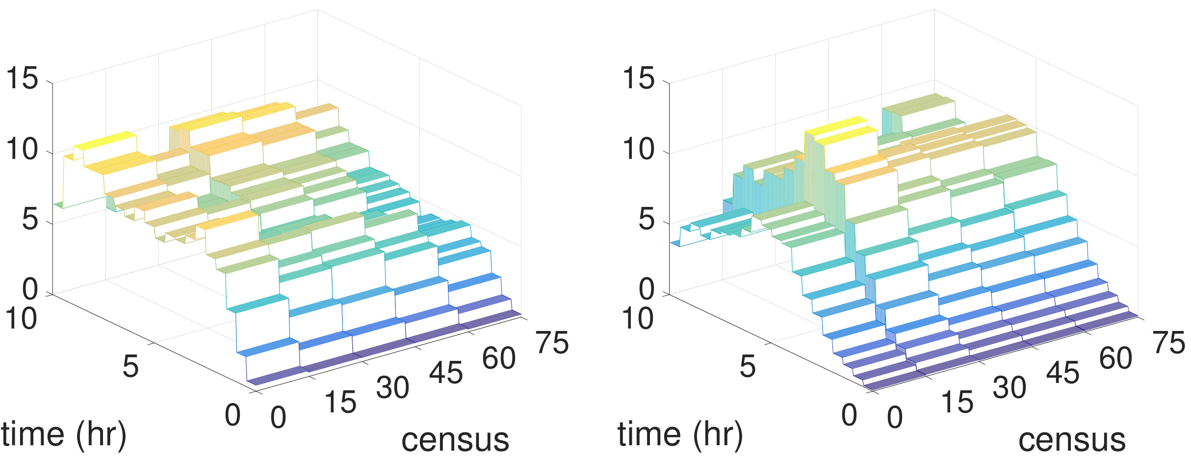 Figure 2
 Figure 3
 Figure 4
 Figure 5
| Time | Age | ESI | Census | All other variables | |
| 0 | 1 | 0.21 | 0.025 | 0.0011 | <0.0010 |
| 1 | 1 | 0.22 | 0.013 | 0.46 | <0.0003 |
| 2 | 0.34 | 0.064 | 0.0020 | 1 | 0 |
| 3 | 0.11 | 0.011 | <0.0001 | 1 | 0 |
| blackboost | Transformation forest | Boosted hazards | Ad-hoc | |
| (set to true log- | (set to true log- | ( fixed for | (# splits fixed | |
| normal distribution) | normal distribution) | all iterations) | for all iterations) | |
| 0 | 5.0% | 5.0% | 7.8% | 7.1% |
| 1 | 17% | 6.1% | 4.5% | 8.1% |
| 2 | 46% | 9.7% | 5.4% | 7.0% |
| 3 | 67% | 18% | 7.2% | 7.4% |
Peer Reviews
No public reviews on file for this paper yet. If you reviewed it on a platform where reviews are public (OpenReview, ICLR, NeurIPS, ICML), you can paste yours below so the community can read it here.
Videos
No videos yet. Explain this paper in a talk, walkthrough, or lecture? Add one.
Boosted nonparametric hazards with time-dependent covariatesDonald K.K. Lee111Correspondence: [email protected]. Supported by a hyperplane, Ningyuan Chen222Supported by the HKUST start-up fund R9382, Hemant Ishwaran333Supported by the NIH grant R01 GM125072Emory University, University of Toronto, University of Miami
Preprint of Annals of Statistics 49:4:2101-2128 (2021)
Given functional data from a survival process with time-dependent covariates, we derive a smooth convex representation for its nonparametric log-likelihood functional and obtain its functional gradient. From this we devise a generic gradient boosting procedure for estimating the hazard function nonparametrically. An illustrative implementation of the procedure using regression trees is described to show how to recover the unknown hazard. The generic estimator is consistent if the model is correctly specified; alternatively an oracle inequality can be demonstrated for tree-based models. To avoid overfitting, boosting employs several regularization devices. One of them is step-size restriction, but the rationale for this is somewhat mysterious from the viewpoint of consistency. Our work brings some clarity to this issue by revealing that step-size restriction is a mechanism for preventing the curvature of the risk from derailing convergence. ††MSC 2010 subject classifications. Primary 62N02; Secondary 62G05, 90B22.††Keywords. survival analysis, gradient boosting, functional data, step-size shrinkage, regression trees, likelihood functional.
1 Introduction
Flexible hazard models involving time-dependent covariates are indispensable tools for studying systems that track covariates over time. In medicine, electronic health records systems make it possible to log patient vitals throughout the day, and these measurements can be used to build real-time warning systems for adverse outcomes such as cancer mortality [2]. In financial technology, lenders track obligors’ behaviours over time to assess and revise default rate estimates. Such models are also used in many other fields of scientific inquiry since they form the building blocks for transitions within a Markovian state model. Indeed, this work was partly motivated by our study of patient transitions in emergency department queues and in organ transplant waitlist queues [20]. For example, allocation for a donor heart in the U.S. is defined in terms of coarse tiers [23], and transplant candidates are assigned to tiers based on their health status at the time of listing. However, a patient’s condition may change rapidly while awaiting a heart, and this time-dependent information may be the most predictive of mortality and not the static covariates collected far in the past.
The main contribution of this paper is to introduce a fully nonparametric boosting procedure for hazard estimation with time-dependent covariates. We describe a generic gradient boosting procedure for boosting arbitrary base learners for this setting. Generally speaking, gradient boosting adopts the view of boosting as an iterative gradient descent algorithm for minimizing a loss functional over a target function space. Early work includes Breiman [6, 7, 8] and Mason et al. [21, 22]. A unified treatment was provided by Friedman [13], who coined the term “gradient boosting” which is now generally taken to be the modern interpretation of boosting.
Most of the existing boosting approaches for survival data focus on time-static covariates and involve boosting the Cox proportional hazards model. Examples include the popular R-packages mboost (Bühlmann and Hothorn [10]) and gbm (Ridgeway [26]) which apply gradient boosting to the Cox partial likelihood loss. Related work includes the penalized Cox partial likelihood approach of Binder and Schumacher [4]. Other important approaches, but not based on the Cox model, include Boosting [11] with inverse probability of censoring weighting (IPCW) [17], boosted transformation models of parametric families [15], and boosted accelerated failure time models [18, 27].
While there are many boosting methods for dealing with time-static covariates, the literature is far more sparse for the case of time-dependent covariates. In fact, to our knowledge there is no general nonparametric approach for dealing with this setting. This is because in order to implement a fully nonparametric estimator, one has to contend with the issue of identifying the gradient, which turns out to be a non-trivial problem due to the functional nature of the data. This is unlike most standard applications of gradient boosting where the gradient can easily be identified and calculated.
*1.1. Time-dependent covariate framework. * To explain why this is so challenging, we start by formally defining the survival problem with time-dependent covariates. Our description follows the framework of Aalen [1]. Let denote the potentially unobserved failure time. Conditional on the history up to time the probability of failing at equals
[TABLE]
Here denotes the unknown hazard function, is a predictable covariate process, and is a predictable indicator of whether the subject is at risk at time .111The filtration of interest is . If is only observable when , we can set whenever . To simplify notation, without loss of generality we normalize the units of time so that for .222Since the data is always observed up to some finite time, there is no information loss from censoring at that point. For example, if is the failure time in minutes and the longest duration in the data is minutes, the failure time in hours, , is at most hour. The hazard function on the minute timescale, , can be recovered from the hazard function on the hourly timescale, , via . In other words, the subject is not at risk after time , so we can restrict attention to the time interval .
If failure is observed at then the indicator equals 1; otherwise and we set to an arbitrary number larger than 1, e.g. . Throughout we assume we observe independent and identically distributed functional data samples . The evolution of observation ’s failure status can then be thought of as a sequence of coin flips at time increments , with the probability of “heads” at each time point given by (1). Therefore, observation ’s contribution to the likelihood is
[TABLE]
where the limit can be understood as a product integral. Hence, if the log-hazard function is
[TABLE]
then the (scaled) negative log-likelihood functional is
[TABLE]
which we shall refer to as the likelihood risk. The goal is to estimate the hazard function nonparametrically by minimizing .
*1.2. The likelihood does not have a gradient in generic function spaces. * As mentioned, our approach is to boost using functional gradient descent. However, the chief difficulty is that the canonical representation of the likelihood risk functional does not have a gradient. To see this, observe that the directional derivative of (2) equals
[TABLE]
which is the difference of two different inner products where
[TABLE]
Hence, (3) cannot be expressed as a single inner product of the form for some function . Were it possible to do so, would then be the gradient function.
In simpler non-functional data settings like regression or classification, the loss can be written as , where is the non-functional statistical target and is the outcome, so the gradient is simply . The negative gradient is then approximated using a base learner from a predefined class of functions (this being either parametric; for example linear learners, or nonparametric; for example tree learners). Typically, the optimal base learner is chosen to minimize the -approximation error and then scaled by a regularization parameter to obtain the updated estimate of :
[TABLE]
Importantly, in the simpler non-functional data setting the gradient does not depend on the space that belongs to. By contrast, a key insight of this paper is that the gradient of can only be defined after carefully specifying an appropriate sample-dependent domain for . The likelihood risk can then be re-expressed as a smooth convex functional, and an analogous representation also exists for the population risk. These representations resolve the difficulty above, allow us to describe and implement a gradient boosting procedure, and are also crucial to establishing guarantees for our estimator.
*1.3. Contributions of the paper. * A key discovery that unlocks the boosted hazard estimator is Proposition 1 of Section 1. It provides an integral representation for the likelihood risk from which several results follow, including, importantly, an explicit representation for the gradient. Proposition 1 relies on defining a suitable space of log-hazard functions defined on the time-covariate domain . Identifying this space is the key insight that allows us to rescue the likelihood approach and to derive the gradient needed to implement gradient boosting. Arriving at this framework is not conceptually trivial, and may explain the absence of boosted nonparametric hazard estimators until now.
Algorithm 1 of Section 1 describes our estimator. The algorithm minimizes the likelihood risk (2) over the defined space of log-hazard functions. In the special case of regression tree learners, expressions for the likelihood risk and its gradient are obtained from Proposition 1, which are then used to describe a tree-based implementation of our estimator in Section 1. In Section 1 we apply it to a high-dimensional dataset generated from a naturalistic simulation of patient service times in an emergency department.
Section 1 establishes the consistency of the procedure. We show that the hazard estimator is consistent if the space is correctly specified. In particular, if the space is the span of regression trees, then the hazard estimator satisfies an oracle inequality and recovers up to some error tolerance (Propositions 3 and 4).
Another contribution of our work is to clarify the mechanisms used by gradient boosting to avoid overfitting. Gradient boosting typically applies two types of regularization to invoke slow learning: (i) A small step-size is used for the update; and (ii) The number of boosting iterations is capped. The number of iterations used in our algorithm is set using the framework of Zhang and Yu [31], whose work shows how stopping early ensures consistency. On the other hand, the role of step-size restriction is more mysterious. While [31] demonstrates that small step-sizes are needed to prove consistency, unrestricted greedy step-sizes are already small enough for classification problems [28] and also for commonly used regression losses (see the Appendix of [31]). We show in Section 1 that shrinkage acts as a counterweight to the curvature of the risk (see Lemma 2). Hence if the curvature is unbounded, as is the case for hazard regression, then the step-sizes may need to be explicitly controlled to ensure convergence. This important result adds to our understanding of statistical convergence in gradient boosting. As noted by Biau and Cadre [3] the literature for this is relatively sparse, which motivated them to propose another regularization mechanism that also prevents overfitting.
Concluding remarks can be found in Section 1. Proofs not appearing in the body of the paper can be found in the Appendix.
2. The boosted hazard estimator. In this section, we describe our boosted hazard estimator. To provide readers with concrete examples for the ideas introduced here, we will show how the quantities defined in this section specialize in the case of regression trees, which is one of a few possible ways to implement boosting.
We begin by defining in Section 1 an appropriate sample-dependent domain for the likelihood risk . As explained, this key insight allows us to re-express the likelihood risk and its population analogue as smooth convex functionals, thereby enabling us to compute their gradients in closed form in Propositions 1 and 2 of Section 1. Following this, the boosting algorithm is formally stated in Section 1.
*2.1. Specifying a domain for . * We will make use of two identifiability conditions (A1) and (A2) to define the domain for . Condition (A1) below is the same as Condition 1(iv) of Huang and Stone [19].
Assumption (A1).
The true hazard function is bounded between some interval on the time-covariate domain .
Recall that we defined and to be predictable processes, and so it can be shown that the integrals and expectations appearing in this paper are all well defined. Denoting the indicator function as , define the following population and empirical sub-probability measures on :
[TABLE]
and note that because the data is i.i.d. by assumption. Intuitively, measures the denseness of the observed sample time-covariate paths on . For any integrable ,
[TABLE]
This allows us to define the following (random) norms and inner products
[TABLE]
and note that because .
By careful design, allows us to specify a natural domain for . Let be a set of bounded functions that are linearly independent, in the sense that if and only if (when some of the covariates are discrete-valued, should be interpreted as the product of a counting measure and the Lebesgue measure). The span of the functions is
[TABLE]
For example, the span of all regression tree functions that can be defined on is ,333It is clear that said span is contained in . For the converse, it suffices to show that is also contained in the span of trees of some depth. This is easy to show for trees with splits, because they can generate partitions of the form in (Section 3 of [8]). which are linear combinations of indicator functions over disjoint time-covariate cubes indexed444With a slight abuse of notation, the index is only considered multi-dimensional when describing the geometry of , such as in (6). In all other situations should be interpreted as a scalar index. by :
[TABLE]
Remark 1.
The regions are formed using all possible split points for the -th coordinate , with the spacing determined by the precision of the measurements. For example, if weight is measured to the closest kilogram, then the set of all possible split points will be kilograms. Note that these split points are the finest possible for any realization of weight that is measured to the nearest kilogram. While abstract treatments of trees assume that there is a continuum of split points, in reality they fall on a discrete (but fine) grid that is pre-determined by the precision of the data.
When is equipped with , we obtain the following sample-dependent subspace of , which is the appropriate domain for :
[TABLE]
Note that the elements in are equivalence classes rather than actual functions that have well defined values at each . This is a problem because the likelihood risk (2) requires evaluating at the points where . We resolve this by fixing an orthonormal basis for , and represent each member of uniquely in the form . For example in the case of regression trees, applying the Gram-Schmidt procedure to gives
[TABLE]
which by design have disjoint support.
The second condition we impose is for to be linearly independent in , that is if and only if . Since by construction are already linearly independent in , the condition intuitively requires the set of all possible time-covariate trajectories to be adequately dense in to intersect a sufficient amount of the support of every . This is weaker than the identifiability conditions 1(ii)-1(iii) in [19] which require to have a positive joint probability density on .
Assumption (A2).
The Gram matrix is positive definite.
*2.2. Integral representations for the likelihood risk. * Having deduced the appropriate domain for , we can now recast the risk as a smooth convex functional on . Proposition 1 below provides closed form expressions for this and its gradient. We note that if the risk is actually of a certain simpler form, it might be possible to estimate its gradient empirically from our risk expression using [24].
Proposition 1.
For functions of the form , the likelihood risk (2) can be written as
[TABLE]
where is the function
[TABLE]
Thus there exists (depending on and ) for which the Taylor representation
[TABLE]
holds, where the gradient
[TABLE]
of is the projection of onto . Hence if then the infimum of over the span of is uniquely attained at .
For regression trees the expressions (7) and (9) simplify further because is closed under pointwise exponentiation, i.e. for . This is because the ’s are disjoint so and hence . Thus
[TABLE]
where
[TABLE]
is the number of observed failures in the time-covariate region .
Proof of Proposition 1.
Fix a realization of . Using (5) we can rewrite (2) as
[TABLE]
We can express in terms of the basis as . Hence
[TABLE]
where the fourth equality follows from the orthonormality of the basis. This completes the derivation of (7).
By an interchange argument we obtain
[TABLE]
the latter being positive whenever ; i.e., is convex. The Taylor representation (8) then follows from noting that is the orthogonal projection of onto . ∎
The expectation of the likelihood risk also has an integral representation. A special case of the representation (13) below is proved in Proposition 3.2 of [19] for right-censored data only, under assumptions that do not allow for internal covariates. In the statement of the proposition below recall that and are defined in (A1). The constant {\alpha_{\!\mathchoice{\raisebox{0.0pt}{\displaystyle{\mathscr{F}}}}{\raisebox{0.0pt}{{\mathscr{F}}}}{\raisebox{-0.85pt}{\scriptstyle{\mathscr{F}}}}{\raisebox{-0.4pt}{\scriptscriptstyle{\mathscr{F}}}}}} is defined later in (28).
Proposition 2.
For ,
[TABLE]
Furthermore the restriction of to is coercive:
[TABLE]
and it attains its minimum at a unique point . If contains the underlying log-hazard function then .
Remark 2.
Coerciveness (14) implies that any with expected risk less than is uniformly bounded:
[TABLE]
where the constant
[TABLE]
is by design no smaller than 1 in order to simplify subsequent analyses.
*2.3. The boosting procedure. * In gradient boosting the key idea is to update an iterate in a direction that is approximately aligned to the negative gradient. To model this direction formally, we introduce the concept of an -gradient.
Definition 1.
Suppose . We say that a unit vector is an -gradient at if for some ,
[TABLE]
Call a negative -gradient if is an -gradient.
Our boosting procedure seeks approximations that satisfy (17) for some pre-specified alignment value . The larger is, the closer the alignment is between the negative gradient and the negative -gradient, and the greater the risk reduction. In particular, is the unique negative 1-gradient with maximal risk reduction. In practice, however, we find that using a smaller value of leads to simpler approximations that prevent overfitting in finite samples. This is consistent with other implementations of boosting: It is well known that the statistical performance of gradient descent generally improves when simpler base learners are used.
Algorithm 1 describes the proposed boosting procedure for estimating . For a given level of alignment , Line 3 finds an -gradient at satisfying (18) at the -th iteration, and uses its negation for the boosting update in Line 4. If the -gradients are tree learners, as is the case with the implementation in Section 1, then the trees cannot be grown in the same way as the standard boosting algorithm in Friedman [13]. This is because the standard approach grows all regression trees to a fixed depth, which may or may not ensure -alignment at each boosting iteration.
To ensure -alignment, the depth of the trees are not fixed in the implementation in Section 1. Instead, at each boosting iteration a tree is grown to whatever depth is needed to satisfy (18). This can always be done because the alignment is non-decreasing in the number of tree splits, and with enough splits we can recover the gradient itself up to -almost everywhere.555Split the tree until each leaf node contains just one of the regions in (6) with . Then set the value of the node equal to the value of the gradient function (12) inside . As mentioned earlier, we recommend using small values of , which can be determined in practice using cross-validation. This differs from the standard approach where cross-validation is used to select a common tree depth to use for all boosting iterations.
In addition to the gradient alignment , Algorithm 1 makes use of two other regularization parameters, and . The first defines the early stopping criterion (how many boosting iterations to use), while the second controls the step-sizes of the boosting updates. These are two common regularization techniques used in boosting:
Early stopping. The number of boosting iterations is controlled by stopping the algorithm before the uniform norm of the estimator reaches or exceeds
[TABLE]
where is the branch of the Lambert function that returns the real root of the equation for . 2. 2.
Step-sizes. The step-size used in gradient boosting is typically held constant across iterations. While we can also do this in our procedure,666The term in condition (20) would need to be replaced by if a constant step-size is used. the role of step-size shrinkage becomes more salient if we use instead as the step-size for the -th iteration in Algorithm 1. This step-size is controlled in two ways. First, it is made to decrease with each iteration according to the Robbins-Monro condition that the sum of the steps diverges while the sum of squared steps converges. Second, the shrinkage factor is selected to make the step-sizes decay with at rate
[TABLE]
This acts as a counterbalance to ’s unbounded curvature:
[TABLE]
which is upper bounded by when and .
3. Consistency. Under (A1) and (A2), guarantees for our hazard estimator in Algorithm 1 can be derived for two scenarios of interest. The guarantees rely on the regularizations described in Section 1 to avoid overfitting. In the following development, recall from Proposition 2 that is the unique minimizer of , so it satisfies the first order condition
[TABLE]
for all . Recall that the span of all trees is closed under pointwise exponentiation (), in which case (22) implies that is the orthogonal projection of onto .
Consistency when is correctly specified. If the true log-hazard function is in , then Proposition 2 asserts that . It will be shown in this case that is consistent:
[TABLE] 2. 2.
Oracle inequality for regression trees. If is closed under pointwise exponentiation, it follows from (22) that is the best -approximation to among all candidate hazard estimators . It can then be shown that converges to this best approximation:
[TABLE]
This oracle result is in the spirit of the type of guarantees available for tree-based boosting in the non-functional data setting. For example, if tree stumps are used for -regression, then the regression function estimate will converge to the best approximation to the true regression function in the span of tree stumps [9]. Similar results also exist for boosted classifiers [5].
Propositions 3 and 4 below formalize these guarantees by providing bounds on the error terms above. While sharper bounds may exist, the purpose of this paper is to introduce our generic estimator for the first time and to provide guarantees that apply across different implementations. More refined convergence rates may exist for a specific implementation, just like the analysis in Bühlmann and Yu [11] for Boosting when componentwise spline learners are specifically used.
En route to establishing the guarantees, Lemma 2 below clarifies the role played by step-size restriction in ensuring convergence of the estimator. As explained in the Introduction, explicit shrinkage is not necessary for classification and regression problems where the risk has bounded curvature. Lemma 2 suggests that it may, however, be needed when the risk has unbounded curvature, as is the case with . Seen in this light, shrinkage is really a mechanism for controlling the growth of the risk curvature.
*3.1. Strategy for establishing guarantees. * The representations for and its population analogue from Section 1 are the key ingredients for formalizing the guarantees. We use them to first show that converges to : Applying Taylor’s theorem to the representation for in Proposition 2 yields
[TABLE]
The problem is thus transformed into one of risk minimization , for which [31] suggests analyzing separately the terms of the decomposition
[TABLE]
The authors argue that in boosting, the point of limiting the number of iterations (enforced by lines 5-10 in Algorithm 1) is to prevent from growing too fast, so that (I) converges to zero as . At the same time, is allowed to grow with in a controlled manner so that the empirical risk in (III) is eventually minimized as . Lemmas 1 and 2 below show that our procedure achieves both goals. Lemma 1 makes use of complexity theory via empirical processes, while Lemma 2 deals with the curvature of the likelihood risk. The term (II) will be bounded using standard concentration results.
*3.2. Bounding (I) using complexity. * To capture the effect of using a simple negative -gradient (17) as the descent direction, we bound (I) in terms of the complexity of777 For technical convenience, has been enlarged from to include the unit ball.
[TABLE]
Depending on the choice of weak learners for the -gradients, may be much smaller than . For example, coordinate descent might only ever select a small subset of basis functions because of sparsity. As another example if is additively separable in time and also in each covariate, then regression trees might only ever select simple tree stumps (one tree split).
The measure of complexity we use below comes from empirical process theory. Define for and suppose that is a sub-probability measure on . Then the -ball of radius centred at some is . The covering number is the minimum number of such balls needed to cover (Definitions 2.1.5 and 2.2.3 of van der Vaart and Wellner [29]), so for . A complexity measure for is
[TABLE]
where the supremum is taken over and over all non-zero sub-probability measures. As discussed, is never greater than, and potentially much smaller than , the complexity of , which is fixed and finite.
Before stating Lemma 1, we note that the result also shows an empirical analogue to the norm equivalences
[TABLE]
exists, where
[TABLE]
The factor of 2 serves to simplify the presentation, and can be replaced with anything greater than 1.
Lemma 1.
There exists a universal constant such that for any , with probability at least
[TABLE]
an empirical analogue to (27) holds for all :
[TABLE]
and for all ,
[TABLE]
Remark 3.
The equivalences (29) imply that equals its upper bound . That is, if , then , so because are linearly independent on .
*3.3. Bounding (III) using curvature. * We use the representation in Proposition 1 to study the minimization of the empirical risk by boosting. Standard results for exact gradient descent like Theorem 2.1.15 of Nesterov [25] are in terms of the norm of the minimizer, which may not exist for .888The infimum of is not always attainable: If is non-positive and vanishes on the set , then is decreasing in so is a direction of recession. This is however not an issue for boosting because of early stopping. If coordinate descent is used instead, Section 4.1 of [31] can be applied to convex functions whose infimum may not be attainable, but its curvature is required to be uniformly bounded above. Since the second derivative of is unbounded (21), Lemma 2 below provides two remedies: (i) Use the shrinkage decay (20) of to counterbalance the curvature; (ii) Use coercivity (15) to show that with increasing probability, are uniformly bounded, so the curvatures at those points are also uniformly bounded. Lemma 2 combines both to derive a result that is simpler than what can be achieved from either one alone. In doing so, the role played by step-size restriction becomes clear. The lemma relies in part on adapting the analysis in Lemma 4.1 of [31] for coordinate descent to the case for generic -gradients. The conditions required below will be shown to hold with high probability.
Lemma 2.
Suppose (29) holds and that
[TABLE]
Then the largest gap between and ,
[TABLE]
is bounded by a constant no greater than 2{\alpha_{\!\mathchoice{\raisebox{0.0pt}{\displaystyle{\mathscr{F}}}}{\raisebox{0.0pt}{{\mathscr{F}}}}{\raisebox{-0.85pt}{\scriptstyle{\mathscr{F}}}}{\raisebox{-0.4pt}{\scriptscriptstyle{\mathscr{F}}}}}}\beta_{\Lambda}, and for ,
[TABLE]
Remark 4.
The last term in (32) suggests that the role of the step-size shrinkage is to keep the curvature of the risk in check, to prevent it from derailing convergence. Recall from (21) that describes the curvature of . Thus our result clarifies the role of step-size restriction in boosting functional data.
Remark 5.
Regardless of whether the risk curvature is bounded or not, smaller step-sizes always improve the convergence bound. This can be seen from the parsimonious relationship between and (32). Fixing , pushing the value of down towards zero yields the lower limit
[TABLE]
However, this limit is unattainable as must be positive in order to decrease the risk. This effect has been observed in practical applications of boosting. Friedman [13] noted improved performance for gradient boosting with the use of a small shrinkage factor . At the same time, it was also noted there was diminishing performance gain as became very small, and this came at the expense of an increased number of boosting iterations. This same phenomenon has also been observed for Boosting [11] with componentwise linear learners. It is known that the solution path for Boosting closely matches that of lasso as . However, the algorithm exhibits cycling behaviour for small , which greatly increases the number of iterations and offsets the performance gain in trying to approximate the lasso (see Ehrlinger and Ishwaran [12]).
*3.4. Formal statements of guarantees. * As a reminder, we have defined the following quantities:
[TABLE]
To simplify the results, we will assume that and also set the shrinkage to satisfy . Our first guarantee shows that our hazard estimator is consistent if the model is correctly specified.
Proposition 3.
(Consistency under correct model specification). Suppose contains the true log-hazard function . Then with probability
[TABLE]
we have that is bounded and
[TABLE]
Thus is consistent.
Via the tension between and , Proposition 3 captures the trade-off in statistical performance between weak and strong learners in gradient boosting. The advantage of low complexity (weak learners) is reflected in the increased probability of the -bound holding, with this probability being maximized when , which generally occurs as . However, diametrically opposed to this, we find that the -bound is minimized by , which occurs with the use of stronger learners that are more aligned with the gradient. This same trade-off is also captured by our second guarantee which establishes an oracle inequality for tree learners.
Proposition 4.
(Oracle inequality for tree learners). Suppose for . Then among , is the best -approximation to , that is
[TABLE]
Moreover, converges to this best approximation : With probability
[TABLE]
we have that is bounded and
[TABLE]
where is the smallest error one can achieve from using functions in to approximate .
For tree learners, is constant over each region in (6), and its value equals the local average of over ,
[TABLE]
Hence if the ’s are small, should closely approximate (recall from Remark 1 that the size of the ’s is fixed by the data). To estimate the approximation error in terms of , suppose that is sufficiently smooth, e.g. Hölder continuous for some . Then since ,
[TABLE]
4. A tree-based implementation. Here we describe an implementation of Algorithm 1 using regression trees, whereby the -gradient is obtained by growing a tree to satisfy (18) for a pre-specified .
To explain the tree growing process, first observe that the -th step log-hazard estimator is an additive expansion of CART basis functions. Thus it can be written as
[TABLE]
where is the -th leaf region of the -th tree. Recall from Section 1 that each tree is grown until (18) is satisfied, so the number of leaf nodes can vary from tree to tree. The leaf regions are typically large subsets of the time-covariate space adaptively determined by the tree growing process (to be discussed shortly). Since each leaf region can be further decomposed into the finer disjoint regions in (6), can be rewritten as (33). However, many of these regions will share the same coefficient value, so (33) can be written more compactly as
[TABLE]
where is the union of contiguous regions whose coefficient equals . This smooths the hazard estimator over , thanks to the regularization imposed by limiting the number of trees (early stopping) and also by the use of weak tree learners. This is unlike the unconstrained hazard MLE defined in (10), which can take on a different value in each region , making it prone to overfit the data.
To construct an -gradient with -alignment to defined by (12),
[TABLE]
the tree splits are adaptively chosen to reduce the -approximation error between and . We implement tree splits for both time and covariates. Specifically, suppose we wish to split a leaf region into left and right daughter subregions and , and assign values and to them. For example, a split on the -th covariate could propose left and right daughters such as
[TABLE]
or a split on time could propose regions
[TABLE]
Now note that is constant within each region . We denote its value by where is the centre of . Hence the best split of into and is the one that minimizes
[TABLE]
where
[TABLE]
represents the -th pseudo-response, its covariate and its weight. Thus the splits use a weighted least squares criterion, which can be efficiently computed as usual.
We split the tree until (18) is satisfied, resulting in leaf nodes ( splits). As discussed in Section 1, we can always find a deep enough tree that is an -gradient because with enough splits we can recover the gradient itself. Recall also that a small value of performs best in practice, and this can be chosen by cross-validating on a set of small-sized candidates: For each one we implement Algorithm 1, and we select the one that minimizes the cross-validated risk defined in (11). By contrast, the standard boosting algorithm [13] uses cross-validation to select a common number of splits to use for all trees, which does not ensure that each tree is an -gradient.
Regarding the possible split points for the covariates (34), note that the -th covariate is a time series that is sampled periodically. This yields a set of unique values equal to the union of all of the sampled values for the observations. In direct analogy to non-functional data boosting, we place candidate split points in-between the sorted values in this set. In other words, splits for covariates only occur at values corresponding to the observed data just as in non-functional boosting.
The resolution for the grid of candidate time splits (35) is set equal to the temporal resolution. For example, the covariate trajectories in the simulation in Section 1 are piecewise constant and may change every 0.002 days. Placing the candidate split points at days simplifies the exact computation of because every covariate trajectory is constant between these points. Again, notice that the splits for time only occur at values informed by the observed data.
Putting it together, the setup above leverages our insight in (36) by transforming the survival functional data into the data values , which enables the implementation to proceed like standard gradient boosting for non-functional data. Only the pseudo-response in needs to be updated at each boosting iteration, while the other two do not change. In terms of storage it costs to store , where is the cardinality of the set of candidate time splits.999Each is of dimension and the number of time-covariate regions with is at most . To show the latter, observe that will only have if it is traversed by at least one sample covariate trajectory. Then note that each of the sample covariate trajectories can traverse at most unique regions. Computationally, choosing a new tree split requires testing candidate splits.101010A sample covariate trajectory can have at most unique observed values for the -th covariate , so there are at most candidate splits for . Thus there are candidate splits for covariates. The number of candidate splits on time is obviously . The space and time complexities of the implementation are reasonable given that they are for non-functional data boosting: In the functional data setting, each sample can have up to observations, so functional data samples is akin to samples in a non-functional data setting.
5. Numerical experiment. We now apply the boosting procedure of Section 1 to a high-dimensional dataset generated from a naturalistic simulation. This allows us to compare the performance of our estimator to existing boosting methods. The simulation is of patient service times in an emergency department (ED), and the hazard function of interest is patient service rate in the ED. The study of patient transitions in an ED queue is an important one in healthcare operations, because without a high resolution model of patient flow dynamics, the ED may be suboptimally utilized which would deny patients of timely critical care.
*5.1. Service rate. * The service rate model used in the simulation is based upon a service time dataset from the ED of an academic hospital in the United States. The dataset contains information on 86,983 treatment encounters from 2014 to early 2015. Recorded for each encounter was: Age, gender, Emergency Severity Index (ESI)111111Level 1 is the most severe (e.g., cardiac arrest) and level 5 is the least (e.g., rash). We removed level 1 patients from the dataset because they were treated in a separate trauma bay., time of day when treatment in the ED ward began, day of week of ED visit, and ward census. The last one represents the total number of occupied beds in the ED ward, which varies over the course of the patient’s stay. Hence it is a time-dependent variable. Lastly, we also have the duration of the patient’s stay (service time).
The service rate function is developed from the data in the following way. First, we apply our nonparametric estimator to the data to perform exploratory analysis. We find that:
The key variables affecting the service rate (based on relative variable importance [13]) are ESI, age, and ward census. In addition, two of the most pronounced interaction terms identified by the tree splits are and . 2. 2.
Holding all the variables fixed, the shapes of the estimated service rate function resemble the hazard functions of log-normal distributions. This agrees with the queuing literature that find log-normality to be a reasonable parametric fit for service durations.
Guided by these findings, we specify the service rate for the simulation as a log-normal accelerated failure time (AFT) model, and estimate its parameters from data. This yields the service rate
[TABLE]
where and are the PDF and CDF of the log-normal distribution with log-mean and log-standard deviation . The function captures the dependence of the service rate on the covariates:
[TABLE]
The specification for above is a slight modification of the original estimate, with the free parameter allowing us to study the effect of time-dependent covariates on hazard estimation. When , the service rate does not depend on time-varying covariates, but as increases, the dependency becomes more and more significant. In the data, the ward census never exceeds 70, so we set the capacity of the simulated ED to 70 as well. The operator caps the impact that census can have on the simulated service rate as grows. The irrelevant covariates are added to the data in order to assess how boosting performs in high dimensions. We explicitly include them in (38) to remind ourselves that the simulated data is high-dimensional. Forty of the irrelevant variables are generated synthetically as described in the next subsection, while the rest are variables from the original dataset not used in the simulation.
*5.2. Simulation model. * Using (37) and (38), we simulate a naturalistic dataset of 10,000 patient visit histories. The value of will be varied from 0 to 3 in order to study the impact of time-dependent covariates on hazard estimation. Each patient is associated with a 46-dimensional covariate vector consisting of:
- •
The time-varying ward census. The initial value is sampled from its marginal empirical distribution in the original dataset. To simulate its trajectory over a patient’s stay, for every timestep advance of 0.002 days (3 minutes), a Bernoulli(0.02) random variable is generated. If it is one, then the census is incremented by a normal random variable with zero mean and standard deviation 10. The result is truncated if it lies outside the range , the upper end being the capacity of the ED.
- •
The other five time-static covariates in the original dataset. These are sampled from their marginal empirical distributions in the original dataset. Two of the variables (age and ESI) influence the service rate, while the other three are irrelevant.
- •
An additional forty time-static covariates that do not affect the service rate (irrelevant covariates). Their values are drawn uniformly from [0,1].
We also generate independent censoring times (rounded to the nearest 0.002 days) for each visit from an exponential distribution. For each simulation, the rate of the exponential distribution is set to achieve an approximate target of 25% censoring.
*5.3. Comparison benchmarks. * When the covariates are static in time, a few software packages are available for performing hazard estimation with tree ensembles. Given that the data is simulated from a log-normal hazard, we compare our nonparametric method to two correctly specified parametric estimators:
The blackboost estimator in the R package mboost [10] provides a tree boosting procedure for fitting the log-normal hazard function. In order to apply this to the simulated data, we make ward census a time-static covariate by fixing it at its initial value. 2. 2.
Transformation forests [16] in the R package trtf can also fit log-normal hazards. Moreover, it allows for left-truncated and right-censored data. Since the ward census variable is simulated to be piecewise constant over time, we can treat each segment as a left-truncated and right-censored observation. Thus for this simulation, transformation forests are able to handle time-dependent covariates with time-static effects. This falls in between the static covariate/static effect blackboost estimator and our fully nonparametric one.
Since the service rate model used in the simulations is in fact log-normal, the benchmark methods above enjoy a significant advantage over our nonparametric one, which is not privy to the true distribution. In fact, when the log-normal hazard (37) depends only on time-static covariates, so the benchmarks should outperform our nonparametric estimator. However, as grows, we would expect a reversal in relative performance.
To compare the performances of the estimators, we use Monte Carlo integration to evaluate the relative mean squared error
[TABLE]
The Monte Carlo integrations are conducted using an independent test set of 10,000 uncensored patient visit histories. For the test set, ward census is held fixed over time at the initial value, and we use the grid for the time integral. The nominator above is then estimated by the average of evaluated at the 5110,000 points of . The denominator is estimated in the same manner.
*5.4. Results. * For the implementation of our estimator in Section 1, the value of and the number of trees are jointly determined using ten-fold cross validation. The candidate values we tried for are , and we limit to no more than 1,000 trees. A wider range of values can be of course be explored for better performance (at the cost of more computations). As comparison, we run an ad-hoc version of our algorithm in which all trees use the same number of splits, as is the case in standard boosting [13]. This approach does not explicitly ensure that the trees will be -gradients for a pre-specified . The number of splits and the number of trees used in the ad-hoc method are jointly determined using ten-fold cross-validation.
In order to speed up convergence at the -th iteration for both approaches, instead of using the step-size of Algorithm 1, we performed line-search within the interval . While Lemma 2 shows that a smaller shrinkage is always better, this comes at the expense of a larger and hence computation time. For simplicity we set for all the experiments here.
For fitting the blackboost estimator, we use the default setting of nu for the step-size taken at each iteration. The other hyperparameters, mstop (the number of trees) and maxdepth (maximum depth of trees), are chosen to directly minimize the relative MSE on the test set. This of course gives the blackboost estimator an unfair advantage over our estimator, which is on top of the fact that it is based on the same distribution as the true model. Transformation forest (using also the true distribution) is fit using code kindly provided by Professor T. Hothorn.121212In the code 100 trees are used in the forest, which takes about 700 megabytes to store the fitted object when applied to our simulated data.
Variable selection. The relative importance of variables [13] for our estimator are given in Table 1 for all four cases . The four factors that influence the service rate (38) are explicitly listed, while the irrelevant covariates are grouped together in the last column. When , the service rate does not depend on census, and we see that the importance of census and the other irrelevant covariates are at least an order of magnitude smaller than the relevant ones. As increases, census becomes more and more important as correctly reflected in the table. Across all the cases the importance of the relevant covariates are at least an order of magnitude larger than the others, suggesting that our estimator is able to pick out the influential covariates and largely avoid the irrelevant ones.
Presence of time-dependent covariates. Table 2 presents the relative MSEs for the estimators as the service rate function (38) becomes increasingly dependent on the time-varying census variable. When the service rate depends only on time-static covariates, so as expected, the parametric log-normal benchmarks perform the best when applied to data simulated from a log-normal AFT model.
However, as increases, the service rate becomes increasingly dependent on census. The corresponding performances of both benchmarks deteriorate dramatically, and is handily outperformed by the proposed estimator. We note that the inclusion of just one time-dependent covariate is enough to degrade the performances of the benchmarks, despite the fact that they have the exact same parametric form as the true model.
Finally we find comparable performance among the ad-hoc boosted estimator and our proposed one, although a slight edge goes to the latter especially in the more difficult simulations with larger . The results here demonstrate that there is a place in the survival boosting literature for fully nonparametric methods like this one that can flexibly handle time-dependent covariates.
6. Discussion. Our estimator can also potentially be used to evaluate the goodness-of-fit of simpler parametric hazard models. Since our approach is likelihood-based, future work might examine whether model selection frameworks like those in [30] can be extended to cover likelihood functionals. For this, [10] provides some guidance for determining the effective degrees of freedom for the boosting estimator. The ideas in [32] may also be germane.
The implementation presented in Section 1 is one of many possible ways to implement our estimator. We defer the design of a more refined implementation to future research, along with open-source code.
Acknowledgements. The review team provided many insightful comments that significantly improved our paper. We are grateful to Brian Clarke, Jack Hall, Sahand Negahban, and Hongyu Zhao for helpful discussions. Special thanks to Trevor Hastie for early formative discussions. The dataset used in Section 1 was kindly provided by Dr. Kito Lord.
APPENDIX: PROOFS
Proof of Proposition 2
Proof.
Writing
[TABLE]
we can apply (4) to establish the first part of the integral in (13) when . To complete the representation, it suffices to show that the point process
[TABLE]
has mean , and then apply Campbell’s formula. To this end, write and consider the filtration . Then has the Doob-Meyer form where is a martingale. Hence
[TABLE]
where the last equality follows from (4). Since is predictable because is, the desired result follows if the stochastic integral is a martingale. By Section 2 of Aalen [1], this is true if is square-integrable. In fact, is bounded because is bounded above by (A1). This establishes (13).
Now note that for a positive constant the function is bounded below by both and , hence . Since is non-increasing in , (A1) implies that
[TABLE]
Integrating both sides and using the norm equivalence relation (27) shows that
[TABLE]
The lower bound (14) then follows from the second inequality. The last inequality shows that is coercive on . Moreover the same argument used to derive (8) shows that is smooth and convex on . Therefore a unique minimizer of exists in . Since (A2) implies there is a bijection between the equivalent classes of and the functions in , is also the unique minimizer of in . Finally, since is pointwise bounded below by , for all . ∎
Proof of Lemma 1
Proof.
By a pointwise-measurable argument (Example 2.3.4 of [29]) it can be shown that all suprema quantities appearing below are sufficiently well behaved, so outer integration is not required. Define the Orlicz norm where . Suppose the following holds:
[TABLE]
where is the complexity measure (26), and are universal constants. Then by Markov’s inequality, (30) holds with probability at least , and
[TABLE]
holds with probability at least 1-2\exp[-\{n^{1/2}/({\alpha_{\!\mathchoice{\raisebox{0.0pt}{\displaystyle{\mathscr{F}}}}{\raisebox{0.0pt}{{\mathscr{F}}}}{\raisebox{-0.85pt}{\scriptstyle{\mathscr{F}}}}{\raisebox{-0.4pt}{\scriptscriptstyle{\mathscr{F}}}}}}\kappa^{\prime\prime}J_{{\mathscr{F}}_{\varepsilon}})\}^{2}]. Since {\alpha_{\!\mathchoice{\raisebox{0.0pt}{\displaystyle{\mathscr{F}}}}{\raisebox{0.0pt}{{\mathscr{F}}}}{\raisebox{-0.85pt}{\scriptstyle{\mathscr{F}}}}{\raisebox{-0.4pt}{\scriptscriptstyle{\mathscr{F}}}}}}>1 and , (30) and (41) jointly hold with probability at least 1-4\exp[-\{\eta n^{1/4}/(\kappa{\alpha_{\!\mathchoice{\raisebox{0.0pt}{\displaystyle{\mathscr{F}}}}{\raisebox{0.0pt}{{\mathscr{F}}}}{\raisebox{-0.85pt}{\scriptstyle{\mathscr{F}}}}{\raisebox{-0.4pt}{\scriptscriptstyle{\mathscr{F}}}}}}J_{{\mathscr{F}}_{\varepsilon}})\}^{2}]. The lemma then follows if (41) implies (29). Indeed, for any non-zero , its normalization is in by construction (25). Then (41) implies that
[TABLE]
because
[TABLE]
where the last inequality follows from the definition of {\alpha_{\!\mathchoice{\raisebox{0.0pt}{\displaystyle{\mathscr{F}}}}{\raisebox{0.0pt}{{\mathscr{F}}}}{\raisebox{-0.85pt}{\scriptstyle{\mathscr{F}}}}{\raisebox{-0.4pt}{\scriptscriptstyle{\mathscr{F}}}}}} (28).
Thus it remains to establish (39) and (40), which can be done by applying the symmetrization and maximal inequality results in Sections 2.2 and 2.3.2 of [29]. Write where are independent copies of the loss
[TABLE]
which is a stochastic process indexed by . As was shown in Proposition 2, . Let be independent Rademacher random variables that are independent of . It follows from the symmetrization Lemma 2.3.6 of [29] for stochastic processes that the left hand side of (39) is bounded by twice the Orlicz norm of
[TABLE]
Now hold fixed so that only are stochastic, in which case the sum in the second line of (1) becomes a separable subgaussian process. Since the Orlicz norm of is bounded by for any constant , we obtain the following the Lipschitz property for any :
[TABLE]
where the second inequality follows from and the last from the Cauchy-Schwarz inequality. Putting the Lipschitz constant obtained above into Theorem 2.2.4 of [29] yields the following maximal inequality: There is a universal constant such that
[TABLE]
where the last line follows from (26). Likewise the conditional Orlicz norm for the supremum of is bounded by . Since neither bounds depend on , plugging back into (1) establishes (39):
[TABLE]
where by (19). On noting that
[TABLE]
(40) can be established using the same approach. ∎
Proof of Lemma 2
Proof.
For , applying (8) to yields
[TABLE]
where the bound for the second term is due to (18) and the bound for the integral follows from (Definition 1 of an -gradient) and for (lines 5-6 of Algorithm 1). Hence for , (44) implies that
[TABLE]
because under (20). Since , and using our assumption in the statement of the lemma, we have
[TABLE]
Clearly the minimizer also satisfies . Thus coercivity (15) implies that
[TABLE]
so the gap defined in (31) is bounded as claimed.
It remains to establish (32), for which we need only consider the case . The termination criterion in Algorithm 1 is never triggered under this scenario, because by Proposition 1 this would imply that minimizes over the span of , which also contains (Remark 3). Thus either , or the termination criterion in line 5 of Algorithm 1 is met. In the latter case
[TABLE]
where the inequalities follow from (29) and from . Since the sum is diverging, the inequality also holds for sufficiently large (e.g. ).
Given that lies in the span of , the Taylor expansion (8) is valid for . Since the remainder term in the expansion is non-negative, we have
[TABLE]
Furthermore for ,
[TABLE]
Putting both into (44) gives
[TABLE]
Subtracting from both sides above and denoting , we obtain
[TABLE]
Since the term inside the first parenthesis is between 0 and 1, solving the recurrence yields
[TABLE]
where in the second inequality we used the fact that for , and the last line follows from (45).
The Lambert function (19) in is asymptotically , and in fact by Theorem 2.1 of [14], for . Since by assumption , the above becomes
[TABLE]
The last step is to control , which is bounded by because . Then under the hypothesis , we have
[TABLE]
Since (14) implies ,
[TABLE]
∎
Proof of Proposition 3
Proof.
Let which is less than one for . Since {\alpha_{\!\mathchoice{\raisebox{0.0pt}{\displaystyle{\mathscr{F}}}}{\raisebox{0.0pt}{{\mathscr{F}}}}{\raisebox{-0.85pt}{\scriptstyle{\mathscr{F}}}}{\raisebox{-0.4pt}{\scriptscriptstyle{\mathscr{F}}}}}},\hat{\gamma}\geq 1 it follows that
[TABLE]
Now define the following probability sets
[TABLE]
and fix a sample realization from . Then the conditions required in Lemma 2 are satisfied with , so (and hence ) is bounded and (32) holds. Since Algorithm 1 ensures that , we have and therefore it also follows that . Combining (23) and (1) gives
[TABLE]
where the second inequality follows from (32) and , and the last from (46). Now, using the inequality yields
[TABLE]
and the stated bound follows from since is correctly specified (Proposition 2).
The next task is to lower bound . It follows from Lemma 1 that
[TABLE]
Bounds on and can be obtained using Hoeffding’s inequality. Note from (2) that and for the loss defined in (42). Since and ,
[TABLE]
By increasing the value of and/or replacing with if necessary, we can combine the inequalities to get a crude but compact bound:
[TABLE]
Finally, since , we can replace in the probability bound above by . ∎
Proof of Proposition 4
Proof.
It follows from (22) that is the orthogonal projection of onto . Hence
[TABLE]
where the inequality follows from . Bounding the last term in the same way as Proposition 3 completes the proof. To replace in (47) by , it suffices to show that . Since the value of over one of its piecewise constant regions is , the desired bound follows from (A1). We can also replace and with and respectively. ∎
REFERENCES
The reference list from the paper itself. Each links out to its DOI / PubMed record.
- 1Aalen [1978] O. O. Aalen. Nonparametric inference for a family of counting processes. Annals of Statistics , 6(4):701–726, 1978.
- 2Adelson et al. [2018] K. Adelson, D. K. K. Lee, S. Velji, J. Ma, S. Lipka, J. Rimar, P. Longley, T. Vega, J. Perez-Irizarry, E. Pinker, and R. Lilenbaum. Development of Imminent Mortality Predictor for Advanced Cancer (IMPAC), a tool to predict short-term mortality in hospitalized patients with advanced cancer. Journal of Oncology Practice , 14(3):e 168–e 175, 2018.
- 3Biau and Cadre [2017] G. Biau and B. Cadre. Optimization by gradient boosting. ar Xiv preprint ar Xiv:1707.05023 , 2017.
- 4Binder and Schumacher [2008] H. Binder and M. Schumacher. Allowing for mandatory covariates in boosting estimation of sparse high-dimensional survival models. BMC Bioinformatics , 9(1):14, 2008.
- 5Blanchard et al. [2003] G. Blanchard, G. Lugosi, and N. Vayatis. On the rate of convergence of regularized boosting classifiers. Journal of Machine Learning Research , 4(Oct):861–894, 2003.
- 6Breiman [1997] L. Breiman. Arcing the edge. U.C. Berkeley Dept. of Statistics Technical Report , 486, 1997.
- 7Breiman [1999] L. Breiman. Prediction games and arcing algorithms. Neural Computation , 11(7):1493–1517, 1999.
- 8Breiman [2004] L. Breiman. Population theory for boosting ensembles. Annals of Statistics , 32(1):1–11, 2004.