New trends in free boundary problems
Serena Dipierro, Aram Karakhanyan, Enrico Valdinoci

TL;DR
This paper reviews recent advances in free boundary problems that incorporate nonlocal interactions or nonlinear energy components, challenging classical assumptions and expanding the scope of the field.
Contribution
It introduces new classes of free boundary problems with nonlocal and nonlinear features, providing novel theoretical insights beyond classical models.
Findings
Identification of nonlocal effects in free boundary problems
Analysis of nonlinear superpositions of energy components
Extension of classical theory to more complex problem classes
Abstract
We present a series of recent results on some new classes of free boundary problems. Differently from the classical literature, the problems considered have either a "nonlocal" feature (e.g., the interaction or/and the interfacial energy may depend on global quantities) or a "nonlinear" flavor (namely, the total energy is the nonlinear superposition of energy components, thus losing the standard additivity and scale invariances of the problem).
Click any figure to enlarge with its caption.
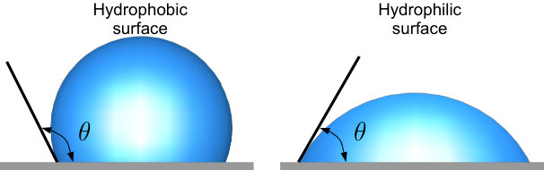 Figure 1
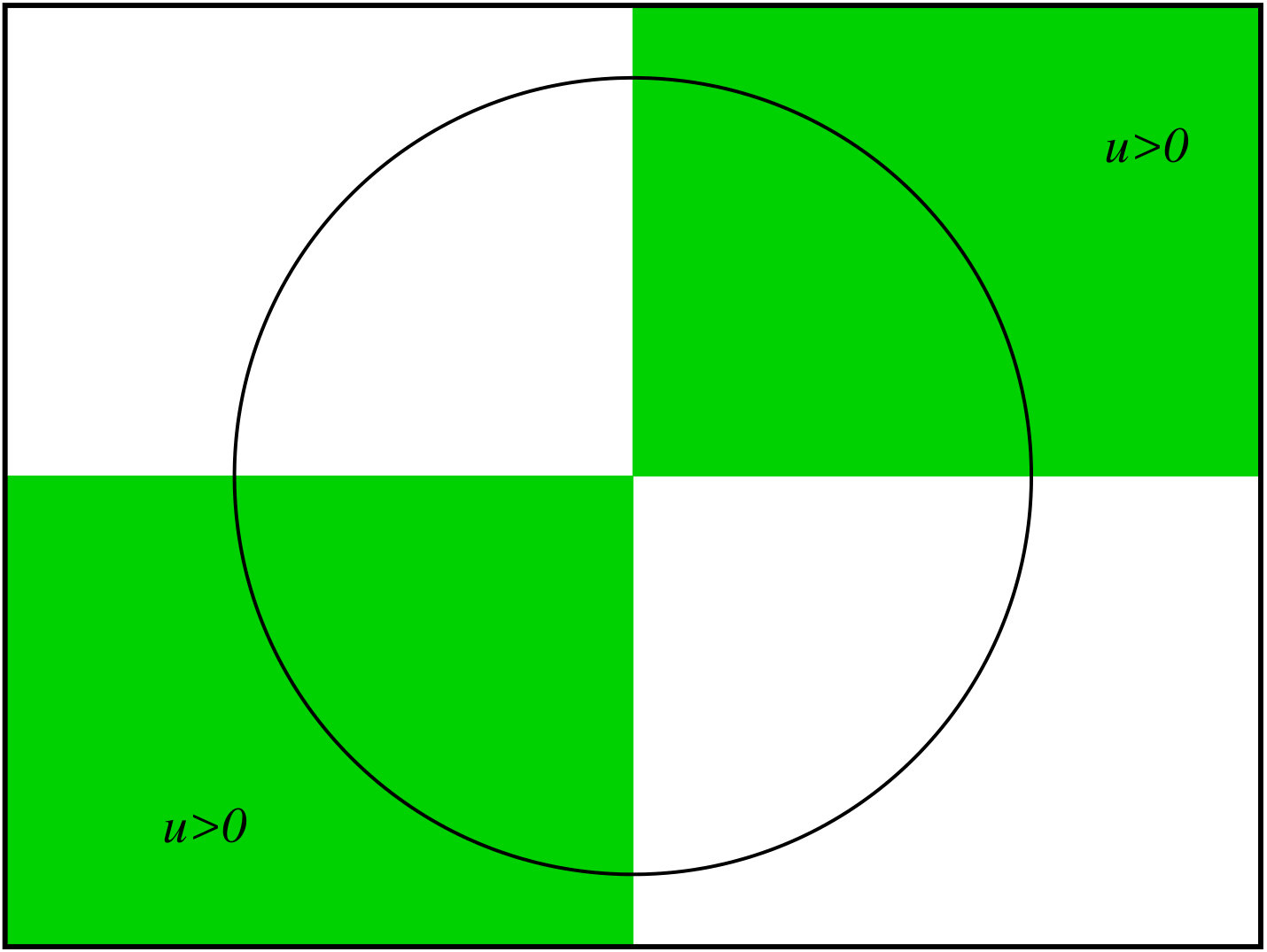 Figure 2
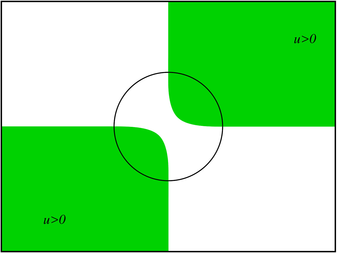 Figure 3
Peer Reviews
No public reviews on file for this paper yet. If you reviewed it on a platform where reviews are public (OpenReview, ICLR, NeurIPS, ICML), you can paste yours below so the community can read it here.
Videos
No videos yet. Explain this paper in a talk, walkthrough, or lecture? Add one.
Taxonomy
TopicsNonlinear Partial Differential Equations · Advanced Mathematical Modeling in Engineering · Differential Equations and Boundary Problems
New trends in free boundary problems
Serena Dipierro
School of Mathematics and Statistics, University of Melbourne, 813 Swanston Street, Parkville VIC 3010, Australia
,
Aram Karakhanyan
Maxwell Institute for Mathematical Sciences and School of Mathematics, University of Edinburgh, James Clerk Maxwell Building, Peter Guthrie Tait Road, Edinburgh EH9 3FD, United Kingdom
and
Enrico Valdinoci
School of Mathematics and Statistics, University of Melbourne, 813 Swanston Street, Parkville VIC 3010, Australia, and Istituto di Matematica Applicata e Tecnologie Informatiche, Consiglio Nazionale delle Ricerche, Via Ferrata 1, 27100 Pavia, Italy, and Weierstraß Institut für Angewandte Analysis und Stochastik, Mohrenstraße 39, 10117 Berlin, Germany, and Dipartimento di Matematica, Università degli studi di Milano, Via Saldini 50, 20133 Milan, Italy
Abstract.
We present a series of recent results on some new classes of free boundary problems. Differently from the classical literature, the problems considered have either a “nonlocal” feature (e.g., the interaction or/and the interfacial energy may depend on global quantities) or a “nonlinear” flavor (namely, the total energy is the nonlinear superposition of energy components, thus losing the standard additivity and scale invariances of the problem).
The complete proofs and the full details of the results presented here are given in [CSV15, DSV15, DV16, DKV15, DKV16, Kar16].
Key words and phrases:
Free boundary problems, nonlocal equations, regularity theory, free boundary conditions, scaling properties, instability.
2010 Mathematics Subject Classification:
35R35, 35R11.
Para Don Ireneo, por supuesto.
1. Introduction
In this survey, we would like to present some recent research directions in the study of variational problems whose minimizers naturally exhibit the formation of free boundaries. Differently than the cases considered in most of the existing literature, the problems that we present here are either nonlinear (in the sense that the energy functional is the nonlinear superposition of classical energy contributions) or nonlocal (in the sense that some of the energy contributions involve objects that depend on the global geometry of the system).
In these settings, the problems typically show new features and additional difficulties with respect to the classical cases. In particular, as we will discuss in further details: the regularity theory is more complicated, there is a lack of scale invariance for some problems, the natural scaling properties of the energy may not be compatible with the optimal regularity, the condition at the free boundary may be of nonlocal or nonlinear type and involve the global behavior of the solution itself, and some problems may exhibit a variational instability (e.g., minimizers in large domains and in small domains may dramatically differ the ones from the others).
We will also discuss how the classical free boundary problems in [AC81, ACF84, ACKS01] are recovered either as limit problems or after a blow-up, under appropriate structural conditions on the energy functional.
We recall the classical free boundary problems of [AC81, ACF84, ACKS01] in Section 2.
The results concerning nonlocal free boundary problems will be presented in Section 3, while the case of nonlinear energy superposition is discussed in Section 4.
2. Two classical free boundary problems
A classical problem in fluid dynamics is the description of a two-dimensional ideal fluid in terms of its stream function, i.e. of a function whose level sets describe the trajectories of the fluid. For this, we consider an incompressible, irrotational and inviscid fluid which occupies a given planar region . If represents the velocity of the particles of the fluid, the incompressibility condition implies that the flow of the fluid through any portions of is zero (the amount of fluid coming in is exactly the same as the one going out), that is, for any , and denoting by the exterior normal vector,
[TABLE]
Since this is valid for any subdomain of , we thus infer that
[TABLE]
Now, we use that the fluid is irrotational to write equation (2.1) as a second order PDE. To this aim, let us analyze what a “vortex” is. Roughly speaking, a vortex is given by a close trajectory, say , along which the fluid particles move. In this way, the velocity field is always parallel to the tangent direction and therefore
[TABLE]
where the standard notation for the circulation line integral is used. That is, if we denote by the region inside enclosed by the curve (hence, ), we infer by (2.2) and Stokes’ Theorem that
[TABLE]
where, as usual, we write to denote the standard basis of , we identify the vector with its three-dimensional image , and
[TABLE]
In this setting, the fact that the fluid is irrotational is translated in mathematical language into the fact that the opposite of (2.3) holds true, namely
[TABLE]
for any (say, with smooth boundary). Since this is valid for any arbitrary region , we thus can translate the irrotational property of the fluid into the condition in , that is
[TABLE]
Now, we consider the -form
[TABLE]
and we have that
[TABLE]
thanks to (2.1). Namely is closed, and thus exact (by Poincaré Lemma, at least if is star-shaped). This says that there exists a function such that
[TABLE]
By comparing this and (2.5), we conclude that
[TABLE]
We observe that is a stream function for the fluid, namely the fluid particles move along the level sets of : indeed, if is the position of the fluid particle at time , we have that is the velocity of the fluid, and
[TABLE]
in view of (2.6).
The stream function also satisfies a natural overdetermined problem. First of all, since represents the boundary of the fluid, and the fluid motion occurs on the level sets of , up to constants we may assume that along . In addition, along Bernoulli’s Law prescribes that the velocity is balanced by the pressure (which we take here to be ). That is, up to dimensional constants, we can write that, along ,
[TABLE]
where we used again (2.6) in the last identity.
Also, (2.4) and (2.6) give that, in ,
[TABLE]
that is, summarizing,
[TABLE]
Notice that these types of overdetermined problems are, in general, not solvable: namely, only “very special” domains allow a solution of such overdetermined problem to exist (see e.g. [Ser71]). In this spirit, determining such domain is part of the problem itself, and the boundary of is, in this sense, a “free boundary” to be determined together with the solution .
These kinds of free boundary problems have a natural formulation, which was widely studied in [AC81, ACF84]. The idea is to consider an energy functional which is the superposition of a Dirichlet part and a volume term. By an appropriate domain variation, one sees that minimizers (or, more generally, critical points) of this functional correspond (at least in a weak sense) to solutions of (2.7) (compare, for instance, the system in (2.7) here with Lemma 2.4 and Theorem 2.5 in [AC81]). Needless to say, in this framework, the analysis of the minimizers of this energy functional and of their level sets becomes a crucial topic of research.
In [ACKS01] a different energy functional is taken into account, in which the volume term is substituted by a perimeter term. This modification provides a natural change in the free boundary condition (in this setting, the pressure of the Bernoulli’s Law is replaced by the curvature of the level set, see formula (6.1) in [ACKS01]).
In the following sections we will discuss what happens when:
- •
we interpolate the volume term of the energy functional of [AC81, ACF84] and the perimeter term of the energy functional of [ACKS01] with a fractional perimeter term, which recovers the volume and the classical perimeter in the limit;
- •
we consider a nonlinear energy superposition, in which the total energy depends on the volume, or on the (possibly fractional) perimeter, in a nonlinear fashion.
3. Nonlocal free boundary problems
A classical motivation for free boundary problems comes from the superposition of a “Dirichlet-type energy” and an “interfacial energy” . Roughly speaking, one may consider the minimization problem of an energy functional
[TABLE]
which takes into account the following two tendencies of the energy contributions, namely:
- •
the term tries to reduce the oscillations of the minimizers,
- •
while the term penalizes the formation of interfaces.
Two classical approaches appear in the literature to measure these interfaces, taking into account the “volume” of the phases or the “perimeter” of the phase separations. The first approach, based on a “bulk” energy contribution, was widely studied in [AC81]. In this setting, the energy superposition in (3.1) (with respect to a reference domain ) takes the form
[TABLE]
where denotes, as customary, the -dimensional Lebesgue measure. The case of two phase contributions (namely, the one which takes into account the bulk energy of both and ) was also considered in [ACF84].
The second approach, based on a “surface tension” energy contribution, was introduced in [ACKS01]. In this setting, the energy superposition in (3.1) takes the form
[TABLE]
where the notation
[TABLE]
represents the perimeter of the set in ; hence, if has smooth boundary, then {\rm Per}(E,\Omega)={\mathscr{H}}^{n-1}\big{(}(\partial E)\cap\Omega\big{)}, being the -dimensional Hausdorff measure.
As pointed out in [CSV15], the two free boundary problems in (3.2) and (3.3) can be settled into a unified framework, and in fact they may be seen as “extremal” problems of a family of energy functionals indexed by a continuous parameter .
To this aim, given two measurable sets , , with , one considers the -interaction of and , as given by the double integral
[TABLE]
In [CRS10a], the notion of -minimal surfaces has been introduced by considering minimizers of the -perimeter induced by such interaction. Namely, one defines the -perimeter of in as the contribution relative to of the -interaction of and its complement (which we denote by ), that is
[TABLE]
After [CRS10a], an intense activity has been performed to investigate the regularity and the geometric properties of -minimal surfaces: see in particular [SV13a, SV13b, CV13, FV15, BFV14] for interior regularity results, and [CDSS16, DSV16b, DSV16a, BLV16] for the rather special behavior of -minimal surfaces near the boundary of the domain. See also [DV17] for a recent survey on -minimal surfaces.
The analysis of the asymptotics of the -perimeter as has been studied under several perspectives in [BBM02, Dáv02, Pon04, CV11, ADPM11, CV13, BN16]. Roughly speaking, up to normalization constants, we may say that approaches the classical perimeter as . On the other hand, as , we have that approaches the Lebesgue measure (again, up to normalization constants, see [MS02, DFPV13, Dip14] for precise statements and examples).
In virtue of these considerations, we have that the free boundary problem introduced in [CSV15], which takes into account the energy superposition in (3.1) of the form
[TABLE]
may be seen as an interpolation of the problems stated in (3.2) and (3.3) (that is, at least at a formal level, the energy functional in (3.5) reduces to that in (3.2) as and to that in (3.3) as ).
A nonlocal variation of the classical Dirichlet energy has been also considered in [CRS10b, DSR12]. In this setting, the classical -seminorm in of a function is replaced by a Gagliardo -seminorm of the form
[TABLE]
where
[TABLE]
and . More precisely, in [CRS10b, DSR12] a superposition of the Gagliardo seminorm and the Lebesgue measure of the positivity set is taken into account.
It is worth to point out that the domain in (3.6) comprises all the interactions of points which involve the domain , since .
In this sense, the integration over is the natural counterpart of the classical integration over of the standard Dirichlet energy, since .
Also, the double integral in (3.6) recovers the classical Dirichlet energy, see e.g. [BBM02, DNPV12].
In this spirit, in [DSV15, DV16] a fully nonlocal counterpart of the free boundary problems in (3.2) and (3.3) has been introduced, by studying energy superpositions of Gagliardo norms and fractional perimeters (see also [DLV] for the superpositions of Gagliardo norms and classical perimeters). More precisely, the energy superposition in (3.1) considered in [DSV15, DV16] takes the form
[TABLE]
where , .
We summarize here a series of results recently obtained in [CSV15, DSV15, DV16] for these nonlocal free boundary problems (some of these results also rely on a notion of fractional harmonic replacement analyzed in [DV15]). First of all, we have that minimizers111Here, for simplicity, we omit the fact that, in this setting, the minimization is performed not only on a function, but on a couple given by the function and its positivity set. See Section 2 in [CSV15] for a rigorous discussion on this important detail. of free boundary problems with fractional perimeter interfaces are continuous, possess suitable density estimates and have smooth free boundaries up to sets of codimension 3:
Theorem 3.1**.**
[Theorems 1.1 and 1.2 in [CSV15]] Let be a minimizer of
[TABLE]
with and .
Then is locally and, for any ,
[TABLE]
for some .
Moreover, the free boundary is a -hypersurface possibly outside a small singular set of Haussdorff dimension .
We remark that the Hölder exponent is consistent with the natural scaling of the problem (namely is still a minimizer). Such type of regularity approaches the optimal exponent in [AC81, ACF84] as . Nevertheless, as , minimizers in [ACKS01] are known to be Lipschitz continuous, therefore we think that it is a very interesting open problem to investigate the optimal regularity of in Theorem 3.1 (we stress that this optimal regularity may well approach the Lipschitz regularity and so “beat the natural scaling of the problem”).
Also, we think it is very interesting to obtain optimal bounds on the dimension of the singular set in Theorem 3.1.
It is also worth to observe that the minimizers in Theorem 3.1 satisfy a nonlocal free boundary condition. Namely, the normal jump along the smooth points of the free boundary coincides (up to normalizing constants) with the nonlocal mean curvature of the free boundary, which is defined by
[TABLE]
for .
This free boundary condition has been presented in formula (1.6) of [CSV15]. Since approaches the classical mean curvature as and a constant as (see e.g. [AV14] and Appendix B of [DV17]), we remark that this nonlocal free boundary condition recovers the classical ones in [ACKS01] and in [AC81, ACF84] as , and as , respectively.
In [DSV15, DV16], we consider the fully nonlocal case in which both the energy components become of nonlocal type, namely we replace (3.8) with the energy functional
[TABLE]
with , , where the notation in (3.7) has been also used.
In this setting, we have:
Theorem 3.2**.**
[Theorem 1.1 in [DV16]] Let be a minimizer of (3.10) with .
Assume that in and that
[TABLE]
Then, is locally and, for any ,
[TABLE]
for some .
We observe that the Hölder exponent in Theorem 3.2 recovers that of Theorem 3.1 as . Once again, we think that it would be very interesting to investigate the optimal regularity of the minimizers in Theorem 3.2. Also, Theorem 3.2 has been established in the “one-phase” case, i.e. under the assumption that the minimizer has a sign. It would be very interesting to establish similar results in the “two-phase” case in which minimizers can change sign. It is worth to remark that the case in which minimizers change sign is conceptually harder in the nonlocal setting than in the local one, since the two phases interact between each other, thus producing additional energy contributions which need to be carefully taken into account.
4. Nonlinear free boundary problems
In [DKV15, DKV16] a new class of free boundary problems has been considered, by taking into account “nonlinear energy superpositions”. Namely, differently than in (3.1), the total energy functional considered in [DKV15, DKV16] is of the form
[TABLE]
for a suitable function . When is linear, the energy functional in (4.1) boils down to its “linear counterpart” given in (3.1), but for a nonlinear function the minimizers of the energy functional in (4.1) may exhibit222Let us give a brief motivation for the nonlinear interface case. The classical energy functionals in [AC81, ACF84, ACKS01] may be also considered in view of models arising in population dynamics. Namely, one can consider the regions and as areas occupied by two different populations, that have reciprocal “hostile” feelings. Then, the diffusive behavior of the populations (which is encoded by the Dirichlet term of the energy) is influenced by the fact that the two populations will have the tendency to minimize the contact between themselves, and so to reduce an interfacial energy as much as possible. In this setting, it is natural to consider the case in which the reaction of the populations to the mutual contact occurs in a nonlinear way. For instance, the case in which additional irrationally motivated hostile feelings arise from further contacts between the populations is naturally modeled by a superlinear interfacial energy, while the case in which the interactions between the populations favor the possibility of compromises and cultural exchanges is naturally modeled by a sublinear interfacial energy. interesting differences with respect to the classical case.
A detailed analysis of free boundary problems as in (4.1) is given in [DKV15, DKV16]. Here, we summarize some of the results obtained (we give here simpler statements, referring to [DKV15, DKV16] for more general results). We take to be monotone, nondecreasing, lower semicontinuous and coercive – in the sense that
[TABLE]
We will also use the notation of writing for every , with the convention that
- •
when , is the nonlocal perimeter defined in (3.4);
- •
when , is the classical perimeter;
- •
when , .
Then, in the spirit of (4.1), we consider energy functionals of the form
[TABLE]
Notice that, for and , the energy in (4.2) reduces to that in (3.8). Similarly, for and , the energy in (4.2) boils down to those in [AC81] and [ACKS01], respectively.
When , a particularly interesting case of nonlinearity is given by . Indeed, in this case, the interfacial energy depends on the -dimensional Lebesgue measure, but it scales like an -dimensional surface measure (also, by Isoperimetric Inequality, the energy levels of the functional in [ACKS01] are above those in (4.2)).
We point out that the free boundary problems in (4.2) develop a sort of natural instability, in the sense that minimizers in a large ball, when restricted to smaller balls, may lose their minimizing properties. In fact, minimizers in large and small balls may be rather different from each other:
Theorem 4.1**.**
[Theorem 1.1 in [DKV15]] There exist a nonlinearity and radii such that a minimizer for (4.2) in is not a minimizer for (4.2) in .
The counterexample in Theorem 4.1, which clearly shows the lack333Just to recall the importance of scaling invariances in the classical free boundary problems, let us quote page 114 of [ACF84]: “for (small) balls […] let us assume (see 3.1) ”. of scaling invariance of the problem, is constructed by taking advantage of the different rates of scaling produced by a suitable nonlinear function , chosen to be constant on an interval. Namely, the “saddle function” in the plane is harmonic and therefore minimizes the Dirichlet energy of (4.2). In large balls, the interface of (as well as the ones of its competitors) produces a contribution that lies in the constant part of , thus reducing the minimization problem of (4.2) to the one coming from the Dirichlet contribution, and so favoring itself. Viceversa, in small balls, the interface of produces more (possibly fractional) perimeter than the one of the competitors whose positivity sets do not come to the origin, and this fact implies that is not a minimizer in small balls.
This argument, which is depicted in Figures 4.1 (A) and (B), is rigorously explained in Section 3 of [DKV15].
In spite of this instability and of the lack of self-similar properties of the energy functional, some regularity results for minimizers of (4.2) still hold true, under appropriate assumptions on the nonlinearity (notice that, for with a constant part, Theorem 4.1 would produce the minimizer whose free boundary is a singular cone, see Figure 4.1 (A), hence any regularity result on the free boundary has to rule out this possibility by a suitable assumption on ). In this sense, we have the following results:
Theorem 4.2**.**
[Corollary 1.4 and Theorems 1.5 and 1.6 in [DKV15]] Let , be Lipschitz continuous and strictly increasing. Let be a minimizer of (4.2) in , with on , for some .
Then, . Also, for any ,
[TABLE]
for some .
For , a result similar to that in Theorem 4.2 holds true, in the sense that is Lipschitz, see Theorems 1.3, 8.1 and 9.2 in [DKV16]. Moreover, in this case one obtains additional results, such as the nondegeneracy of the minimizers, the partial regularity of the free boundary and the full regularity in the plane:
Theorem 4.3**.**
[Theorems 1.4, 1.6 and 1.7 in [DKV16]] Let , be Lipschitz continuous and strictly increasing. Let be a minimizer of (4.2) in , with (in the measure theoretic sense).
Then, for any , there exists such that for any for which , it holds that
[TABLE]
Also, is locally BMO, in the sense that
[TABLE]
for some , where
[TABLE]
In addition {\mathcal{H}}^{n-1}\big{(}B_{r}\cap(\partial\{u_{\star}>0\})\big{)}<+\infty.
Finally, if , then is made of continuously differentiable curves.
The BMO-type regularity and the partial regularity of the free boundary in Theorem 4.3 rely in turn on some techniques developed in [DK15].
It is also interesting to remark that the case recovers the classical problems in [AC81] after a blow-up:
Theorem 4.4**.**
[Theorem 1.5 and Proposition 10.1 in [DKV16]] Let , be Lipschitz continuous and strictly increasing. Let be a minimizer of (4.2) in , with .
For any , let . Then, there exists the blow-up limit
[TABLE]
Also, is continuous and with linear growth, and it is a minimizer of the functional
[TABLE]
where
[TABLE]
We stress that the energy functional in (4.3) coincides with that analyzed in the classical paper [AC81]. Nevertheless, the “scaling constant” in (4.3) depends on the original minimizer , as prescribed by (4.4) (only in the case of a linear , we have that is a structural constant independent of ).
The fact that geometric and physical quantities arising in this type of problem are not universal constants but depend on the minimizer itself is, in our opinion, an intriguing feature of this type of problems. In this sense, we recall that in [AC81] the free boundary condition coincides with the classical Bernoulli’s law, namely the normal jump along the smooth points of the free boundary is constant (in [ACKS01] it coincides with the mean curvature of the free boundary). Differently from the classical cases, in our nonlinear setting, the free boundary condition depends on the minimizer itself. Indeed, in our case the normal jump coincides with
[TABLE]
where is the nonlocal mean curvature of the free boundary, as defined in (3.9) (see formula (1.12) in [DKV15] and formulas (1.13) and (1.14) in [DKV16]).
We point out that (4.5) recovers the classical cases in [AC81, ACKS01] when and is linear. On the other hand, when is not linear, the free boundary condition in (4.5) takes into account the global behavior of the free boundary and the (possibly fractional) perimeter of the minimizer in the whole of the domain. In this sense, this type of condition is “self-driven”, since it is influenced by the minimizer itself and not only by the environmental conditions and the structural constants.
5. Regularity of stationary points of the Alt-Caffarelli functional
In this section we would like to discuss some recent results on the further connections between the Alt-Caffarelli problem and the minimal surfaces. More specifically, we consider the stationary points (in particular minimizers) of the functional
[TABLE]
and the capillarity surfaces in the sphere of radius (notice that the critical points of the functional in (5.1) are related to the system in (2.7), see Theorem 2.5 in [AC81] for details on this).
The starting point of our analysis is to study the classical capillary drop problem.
5.1. Capillary drop problem
We first revisit the sessile drop problem and its higher dimensional analogue.
We consider the functional
[TABLE]
where , , is a given constant, , and is the characteristic function of , where
[TABLE]
Here, the parameter is the volume fraction of the droplet.
For , the functional in (5.2) is related to the sessile drop problem, i.e. the problem of a (three-dimensional) capillarity drop occupying the set and sitting in the halfspace
We observe that the first term in is the energy due to the surface tension, the second term is the gravitational energy and the last term is the wetting energy which produces a contact angle such that (see Figure 5.1).
By a Taylor expansion, we see that
[TABLE]
Hence, if is the graph of a (smooth) function (with small gradient), we obtain the approximation
[TABLE]
In other words, the functional in (5.1) is the linearization of the sessile drop problem described by the functional in (5.2), with no gravity and constant wetting energy density. This suggests that there must be a strong link between the regularity of the minimizers of and the minimal surfaces. We will now discuss444For completeness, we recall that a nonlocal capillarity theory has been recently developed in [MV16, DMV16]. in which sense this link rigorously occurs.
5.2. Homogeneity of blow-ups and the support function
The first of such direct links was established in [DSJ09], where it is showed that the singular axisymmetric critical point of is an energy minimizer in dimension 7. This singular energy minimizer of the Alt-Caffarelli problem can be seen as the analog of the Simons cone
[TABLE]
which is an example of a singular hypersurface of least perimeter in dimension . The minimality of the Simons cone was first proved by E. Bombieri, E. De Giorgi and E. Giusti in [BDGG69].
The cones with non-negative mean curvature arise naturally in the blow-up procedure of the minimizer at a free boundary point. By Weiss’ monotonicity formula (see [Wei98]), any blow-up limit of an energy minimizer of is defined on and must be a homogeneous function of degree one.
Let us write
[TABLE]
where (being , as usual, the unit sphere in ). Since is also a global minimizer of then it follows that in . Rewriting the equation in polar coordinates we infer that is a solution of the equation
[TABLE]
Here is the Laplace-Beltrami operator on the sphere. We observe that if and only if and on the free boundary of which is a cone due to the homogeneity of .
Equation (5.4) can be rewritten as
[TABLE]
It is well-known that
[TABLE]
determined by the parameterization
[TABLE]
see [Ale39]. In addition, we have that and the sphere are perpendicular at the contact points, see [Kar16].
In this sense, one can interpret as the Minkowski support function of the surface In other words and it is the distance of the tangent plane with normal from the origin.
5.3. The mean radius equation
The previous discussion tells us that the sum of the principal radii of the surface is zero. Indeed, let be the th principal curvature of and the corresponding principal radius. Then, in view of (5.6), it holds that the matrix has eigenvalues , and so its trace is equal to . From this and (5.5), we thus obtain that
[TABLE]
This is called the mean radius equation. Recalling (5.3), the free boundary condition given in [AC81] (and corresponding to the constancy of ) along now becomes
[TABLE]
This means that the surface is contained in the sphere of radius .
We point out that in dimension formula (5.7) reduces to
[TABLE]
and therefore the mean curvature vanishes whenever the Gauss curvature is nonzero (i.e., ). If , then such simple interpretation is not possible.
In terms of the classification of global cones for the Alt-Caffarelli problem, we recall that the open question is whether for the stable solution of the mean radius equation in such that on is the disk passing through the origin (when , this question is settled in [AC81], the case was addressed in [CJK04] and was proved in [JS15]).
An open and challenging question is to classify the stationary solutions and the corresponding zero mean radius surfaces of given topological type.
5.4. Flame models
A closely related problem is the behavior of the solutions to the singular perturbation problem
[TABLE]
where is small and
[TABLE]
is an approximation of the Dirac measure. It is well known that (5.8) models propagation of equidiffusional premixed flames with high activation of energy, see [Caf95].
The limit (for a suitable sequence ) solves a Bernoulli type free boundary problem with the following free boundary condition
[TABLE]
In fact, it holds that is a stationary point of the Alt-Caffarelli functional in (5.1).
If we choose to be a family of minimizers of the functional
[TABLE]
then inherits the generic features of the Alt-Caffarelli minimizers as described in [AC81, ACF84] (e.g. non-degeneracy, rectifiability of , etc.). Consequently, by sending , one can see that the limit exists and it is a minimizer of the Alt-Caffarelli functional
[TABLE]
As it was mentioned above, the singular set of minimizers is empty in dimensions and . However, if is not a minimizer then not much is known about the classification of the blow-ups of the limit function . An interesting question is to classify these stationary points of given topological type or Morse index. One recent result in this direction is that the associated surface that we constructed via the support function is of ring type then is a piece of catenoid, see [Kar16].
The reference list from the paper itself. Each links out to its DOI / PubMed record.
- 1[AC 81] H. W. Alt and L. A. Caffarelli. Existence and regularity for a minimum problem with free boundary. J. Reine Angew. Math. , 325:105–144, 1981. CODEN JRMAA 8. ISSN 0075-4102.
- 2[ACF 84] Hans Wilhelm Alt, Luis A. Caffarelli, and Avner Friedman. Variational problems with two phases and their free boundaries. Trans. Amer. Math. Soc. , 282(2):431–461, 1984. CODEN TAMTAM. ISSN 0002-9947. URL http://dx.doi.org/10.2307/1999245 .
- 3[ACKS 01] I. Athanasopoulos, L. A. Caffarelli, C. Kenig, and S. Salsa. An area-Dirichlet integral minimization problem. Comm. Pure Appl. Math. , 54(4):479–499, 2001. CODEN CPAMA. ISSN 0010-3640. URL http://dx.doi.org/10.1002/1097-0312(200104)54:4<479::AID-CPA 3>3.3.CO;2-U .
- 4[ADPM 11] Luigi Ambrosio, Guido De Philippis, and Luca Martinazzi. Gamma-convergence of nonlocal perimeter functionals. Manuscripta Math. , 134(3-4):377–403, 2011. CODEN MSMHB 2. ISSN 0025-2611. URL http://dx.doi.org/10.1007/s 00229-010-0399-4 .
- 5[Ale 39] A. Alexandroff. über die Oberflächenfunktion eines konvexen Körpers. (Bemerkung zur Arbeit “Zur Theorie der gemischten Volumina von konvexen Körpern”). Rec. Math. N.S. [Mat. Sbornik] , 6(48):167–174, 1939.
- 6[AV 14] Nicola Abatangelo and Enrico Valdinoci. A notion of nonlocal curvature. Numer. Funct. Anal. Optim. , 35(7-9):793–815, 2014. ISSN 0163-0563. URL http://dx.doi.org/10.1080/01630563.2014.901837 .
- 7[BBM 02] Jean Bourgain, Haïm Brezis, and Petru Mironescu. Limiting embedding theorems for W s , p superscript 𝑊 𝑠 𝑝 W^{s,p} when s ↑ 1 ↑ 𝑠 1 s\uparrow 1 and applications. J. Anal. Math. , 87:77–101, 2002. CODEN JOAMAV. ISSN 0021-7670. URL http://dx.doi.org/10.1007/BF 02868470 . Dedicated to the memory of Thomas H. Wolff.
- 8[BDGG 69] E. Bombieri, E. De Giorgi, and E. Giusti. Minimal cones and the Bernstein problem. Invent. Math. , 7:243–268, 1969. ISSN 0020-9910. URL http://dx.doi.org/10.1007/BF 01404309 .