Study of the $D^0 p$ amplitude in $\Lambda_b^0\to D^0 p \pi^-$ decays
LHCb collaboration: R. Aaij, B. Adeva, M. Adinolfi, Z. Ajaltouni, S., Akar, J. Albrecht, F. Alessio, M. Alexander, S. Ali, G. Alkhazov, P. Alvarez, Cartelle, A.A. Alves Jr, S. Amato, S. Amerio, Y. Amhis, L. An, L. Anderlini,, G. Andreassi, M. Andreotti, J.E. Andrews

TL;DR
This paper performs an amplitude analysis of the decay $ olinebreak ext{Λ}_b^0 o D^0 p ext{π}^-$, measuring properties of excited $ ext{Λ}_c^+$ states, including a potential new resonance, using LHCb data.
Contribution
It provides the first constraints on the spin and parity of the $ ext{Λ}_c(2940)^+$ and reports evidence for a new $ ext{Λ}_c(2860)^+$ resonance.
Findings
Measured masses, widths, and quantum numbers of $ ext{Λ}_c(2880)^+$ and $ ext{Λ}_c(2940)^+$.
First constraints on the spin and parity of $ ext{Λ}_c(2940)^+$.
Evidence for a new $ ext{Λ}_c(2860)^+$ resonance with spin 3/2 and positive parity.
Abstract
An amplitude analysis of the decay is performed in the part of the phase space containing resonances in the channel. The study is based on a data sample corresponding to an integrated luminosity of 3.0 fb of collisions recorded by the LHCb experiment. The spectrum of excited states that decay into is studied. The masses, widths and quantum numbers of the and resonances are measured. The constraints on the spin and parity for the state are obtained for the first time. A near-threshold enhancement in the amplitude is investigated and found to be consistent with a new resonance, denoted the , of spin and positive parity.
Click any figure to enlarge with its caption.
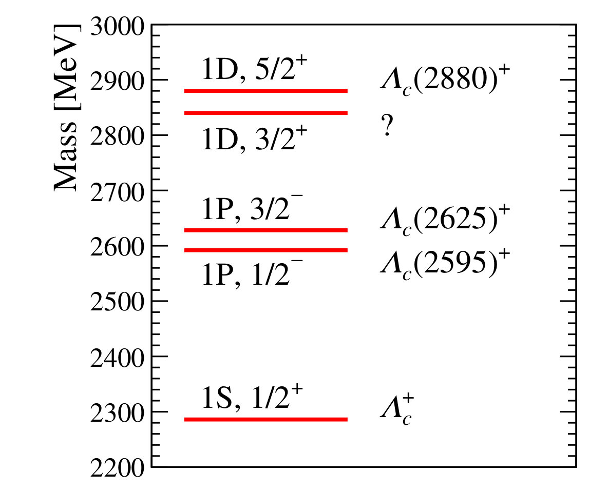 Figure 1
 Figure 10
 Figure 10
 Figure 10
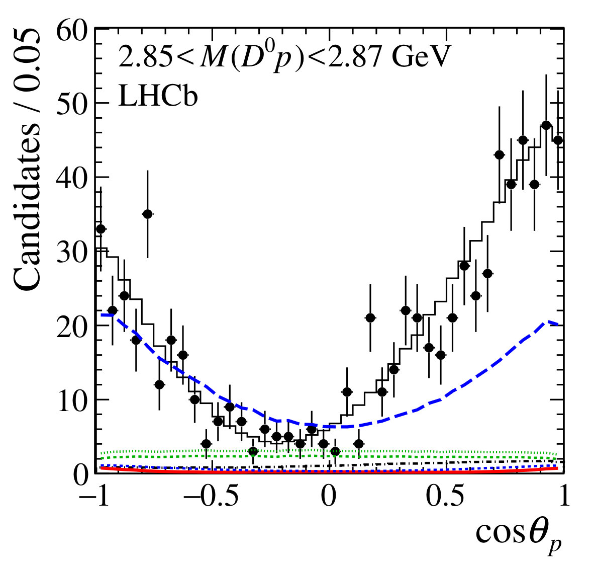 Figure 10
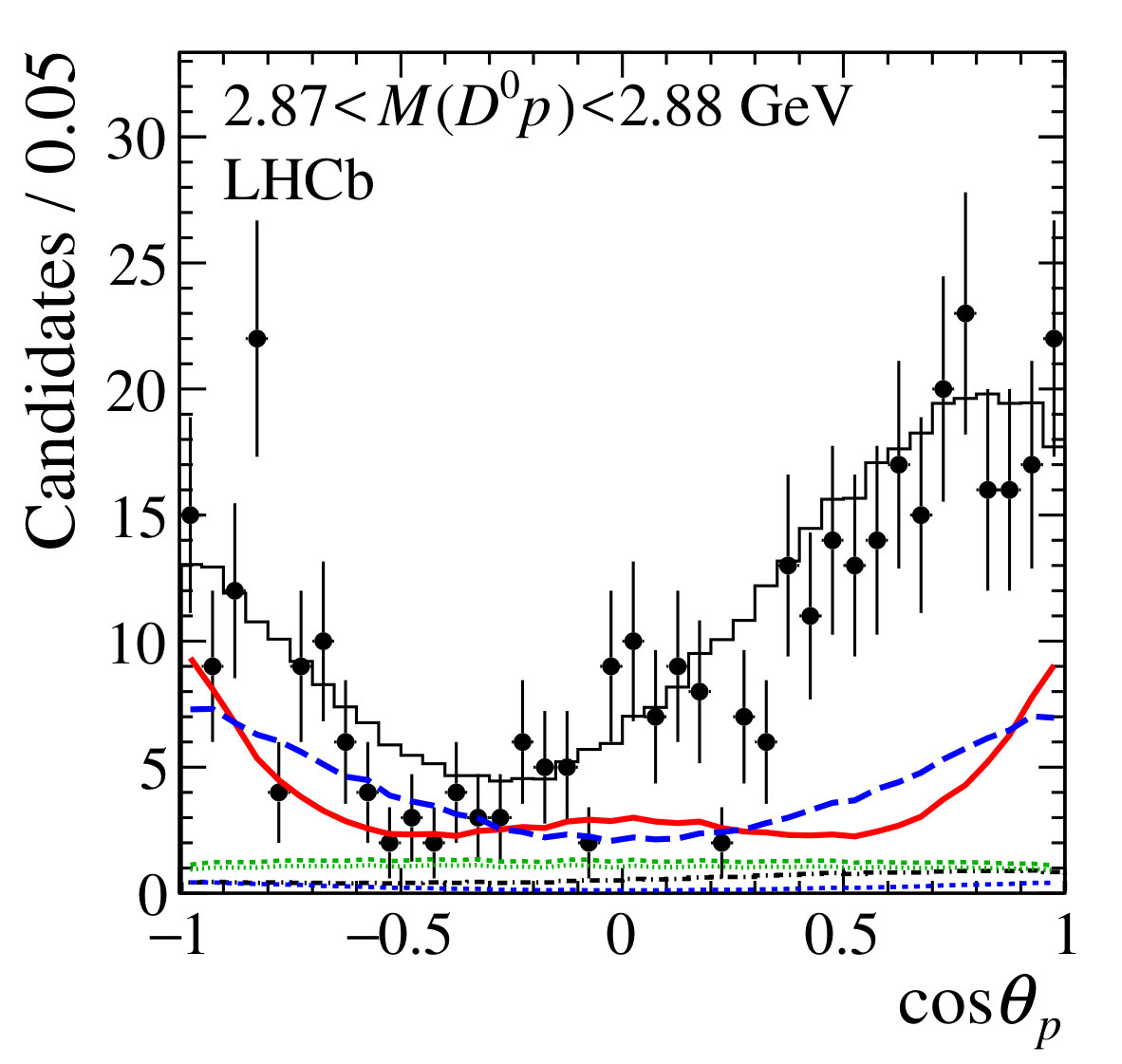 Figure 10
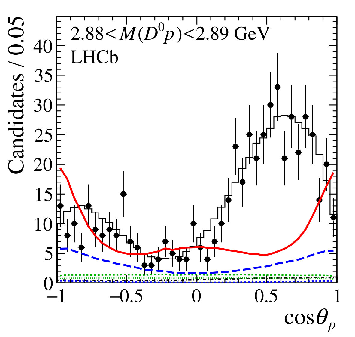 Figure 10
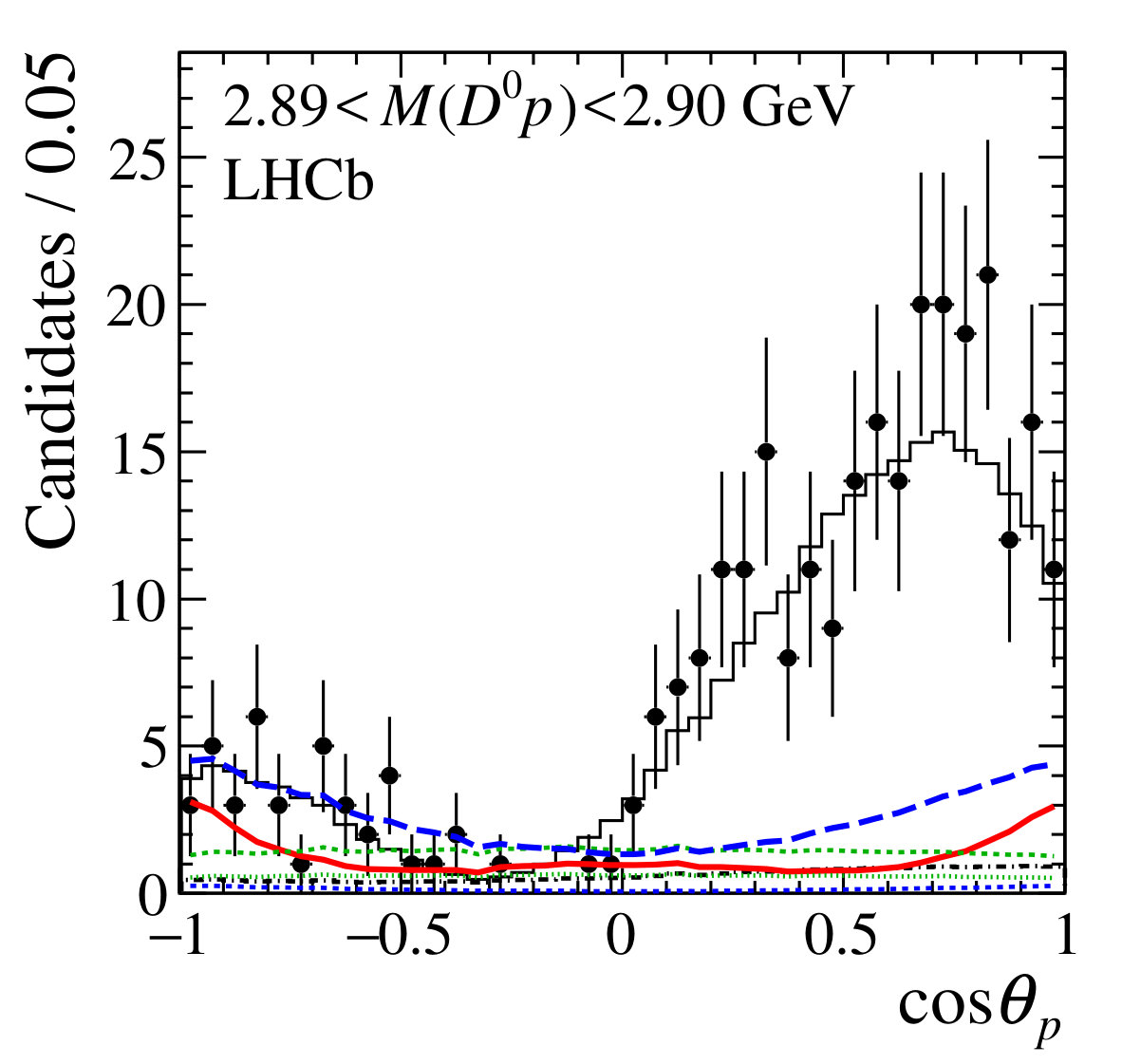 Figure 10
 Figure 10
 Figure 11
 Figure 11
 Figure 12
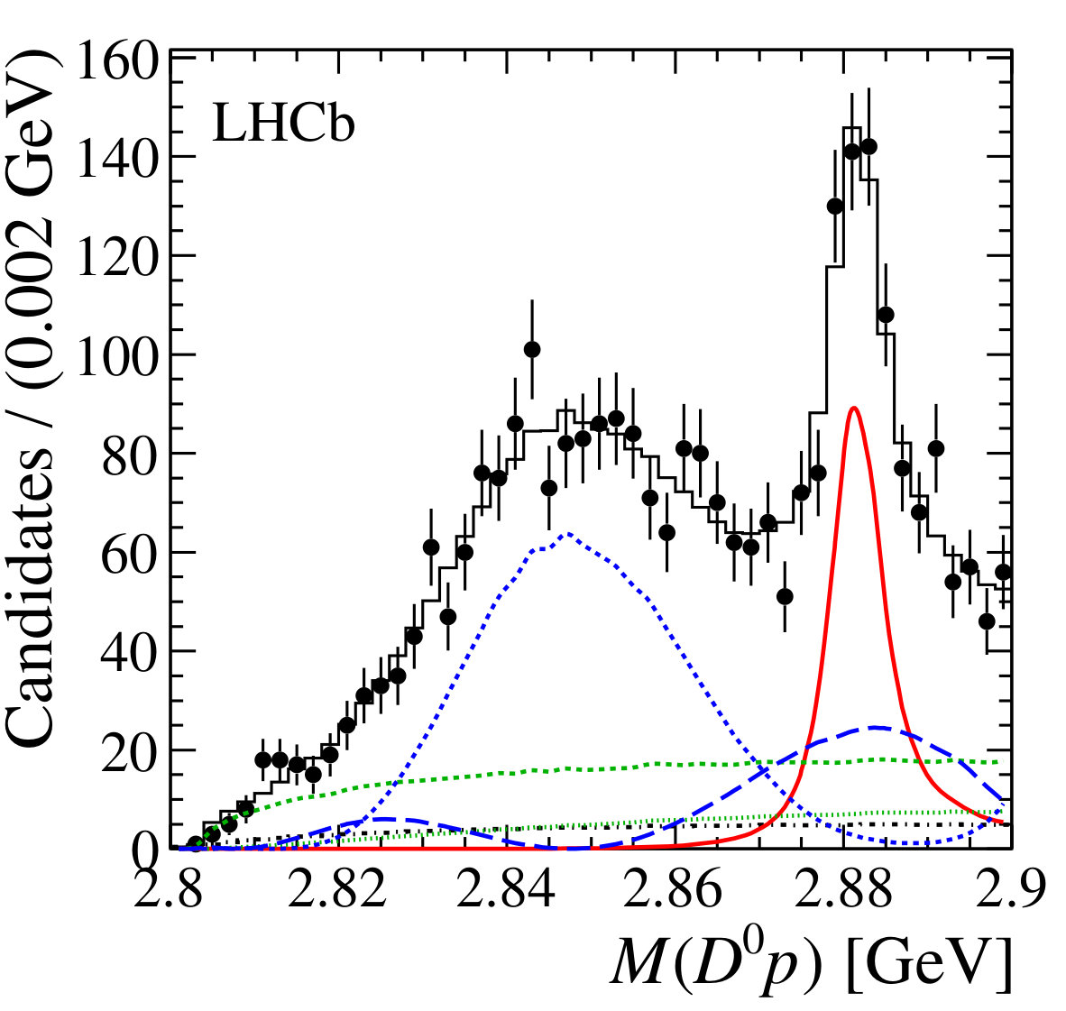 Figure 12
 Figure 12
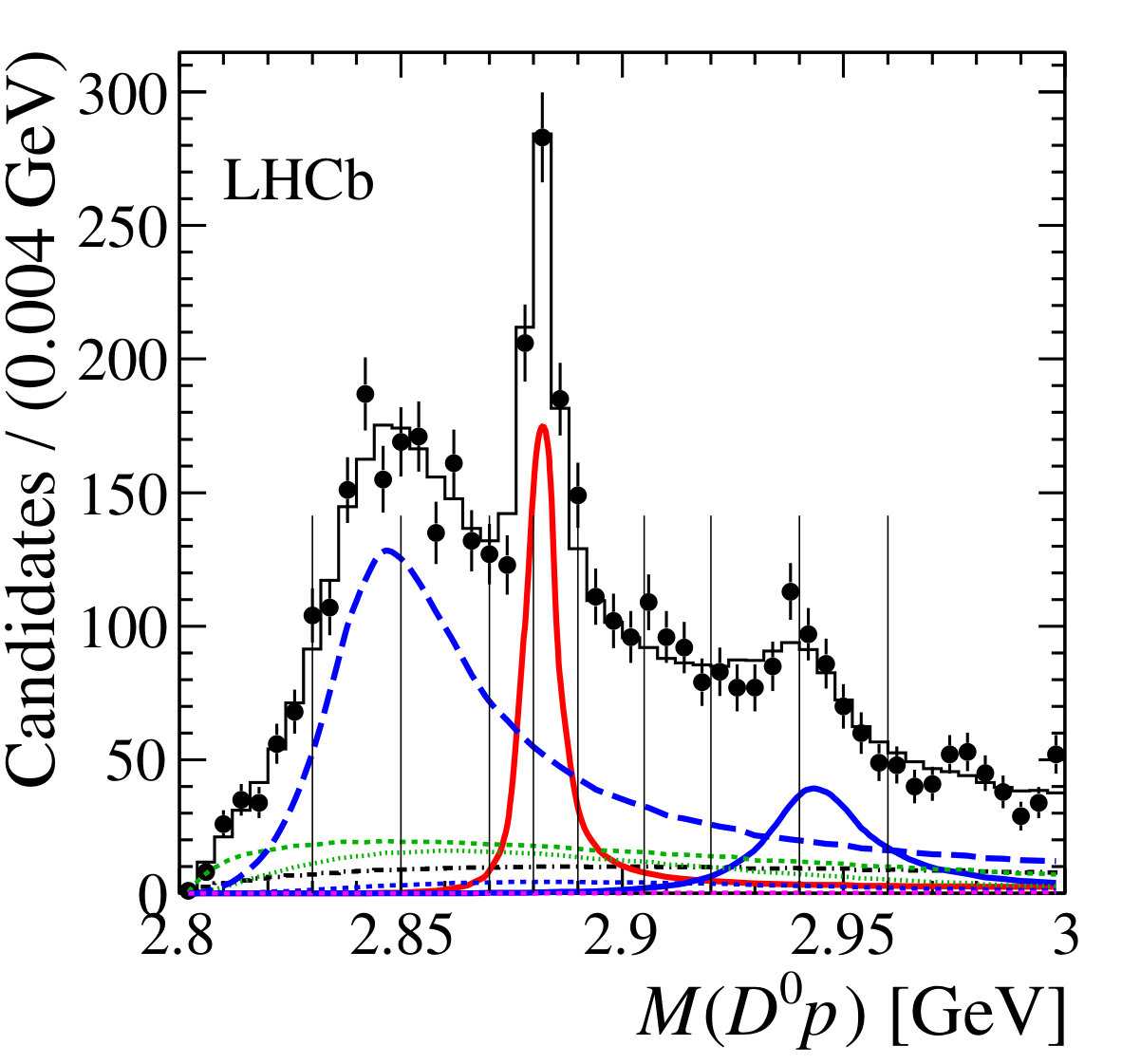 Figure 13
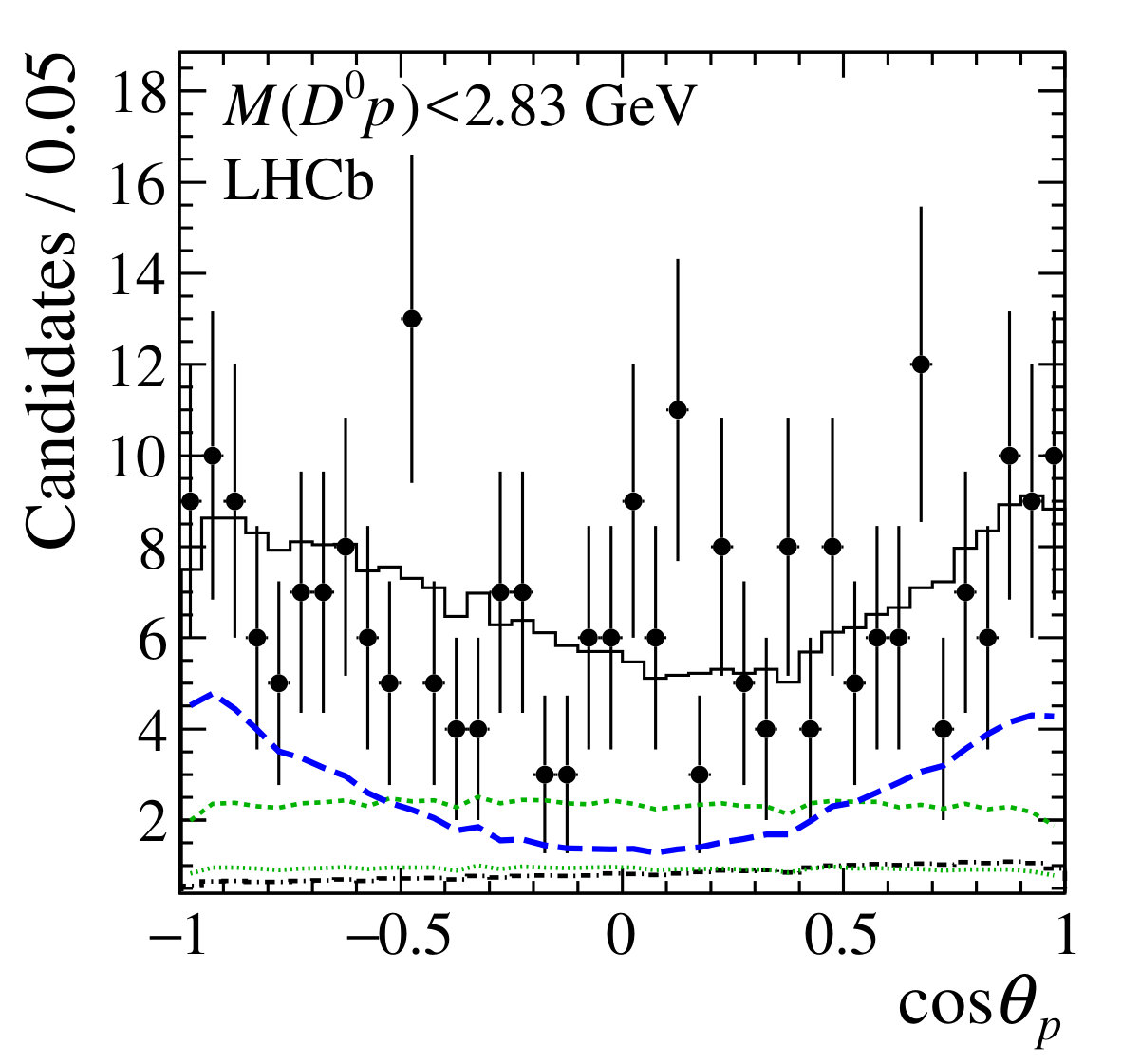 Figure 13
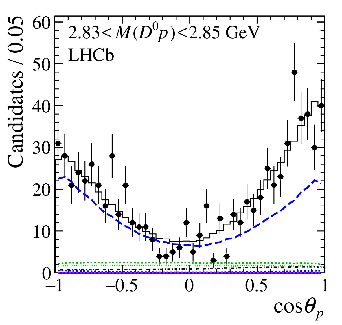 Figure 13
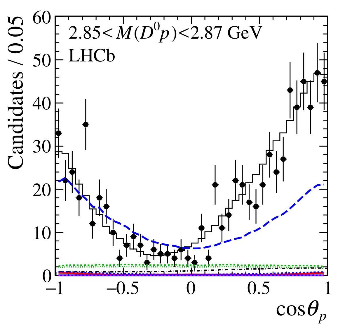 Figure 13
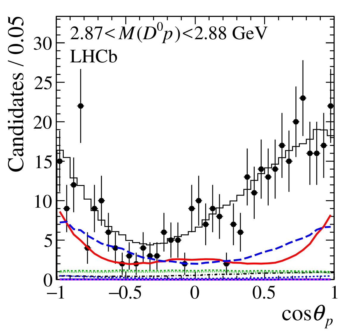 Figure 13
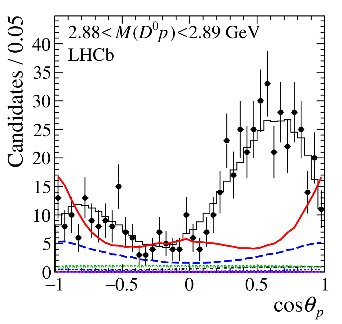 Figure 13
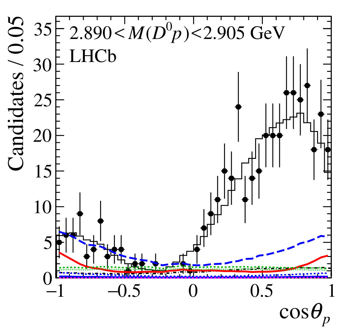 Figure 13
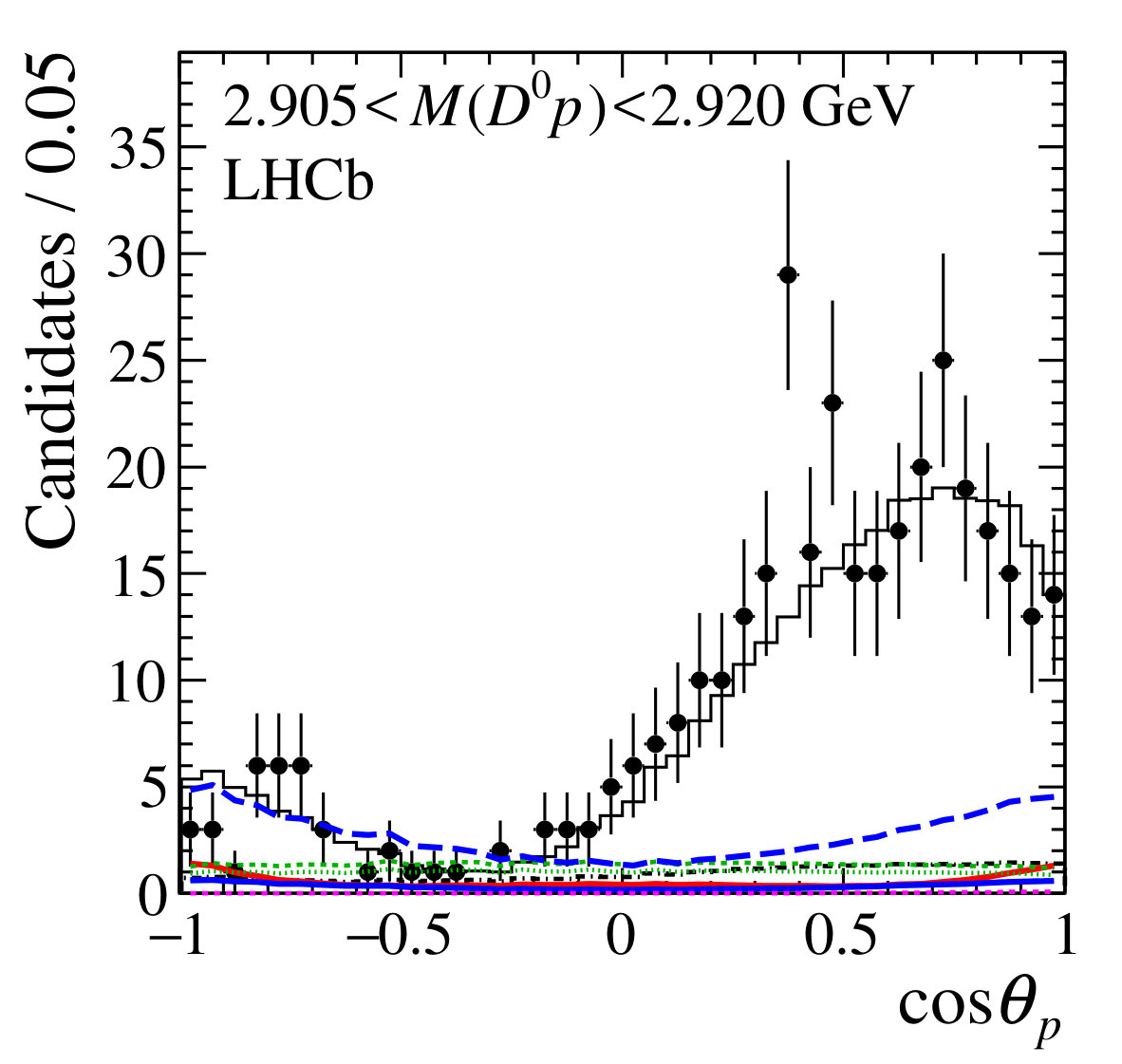 Figure 13
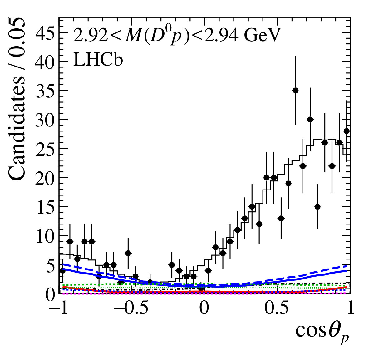 Figure 13
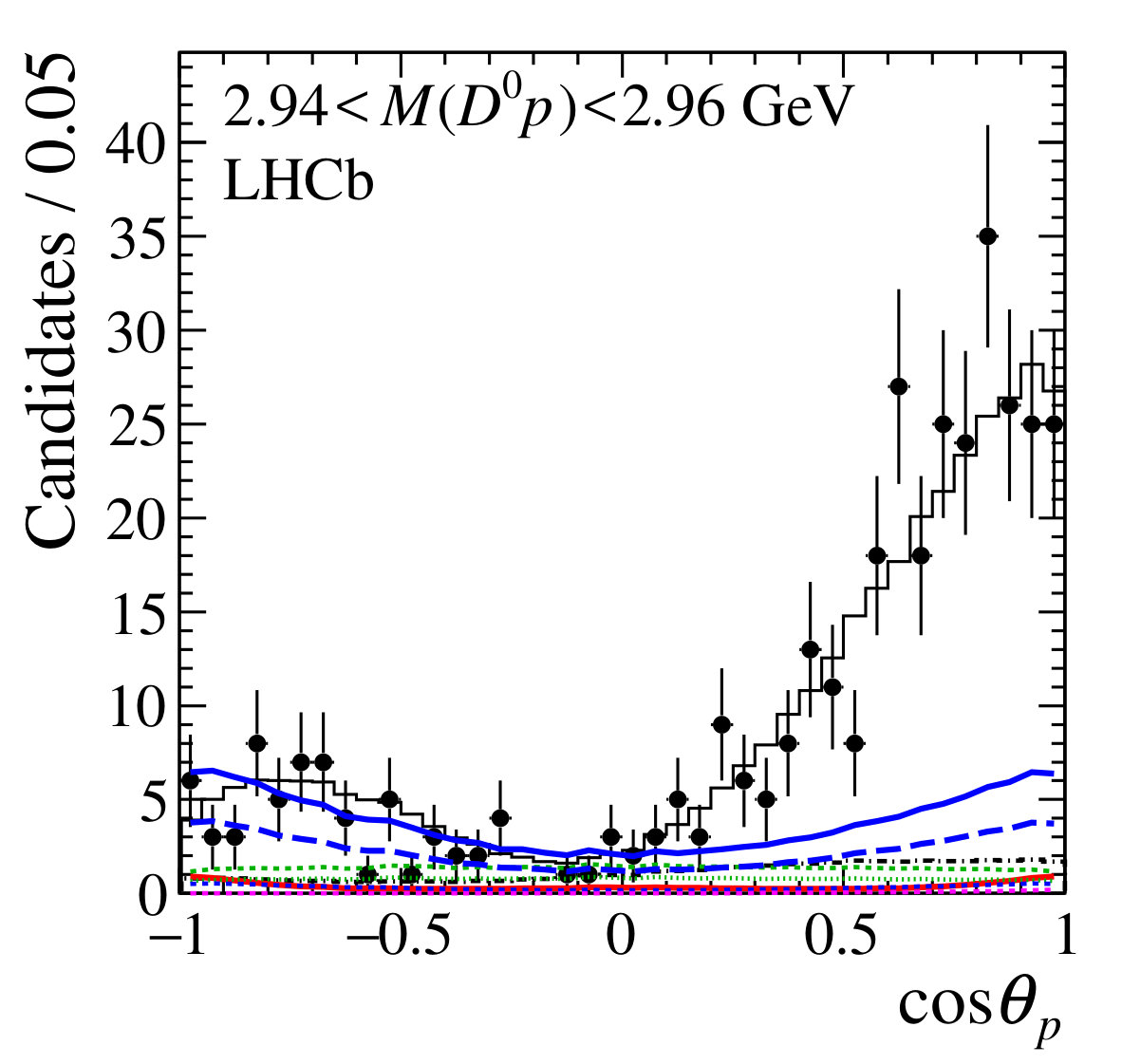 Figure 13
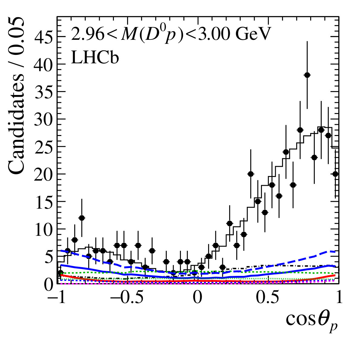 Figure 13
 Figure 13
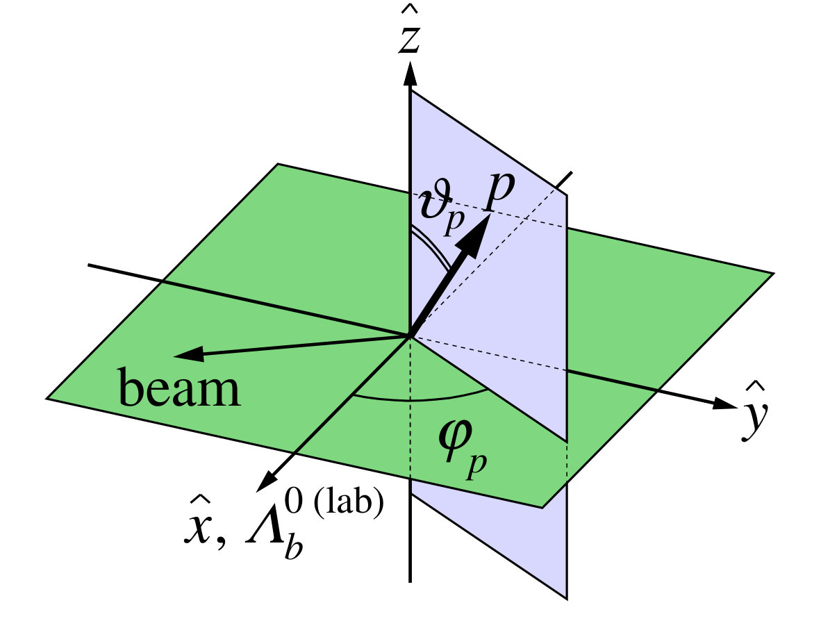 Figure 2
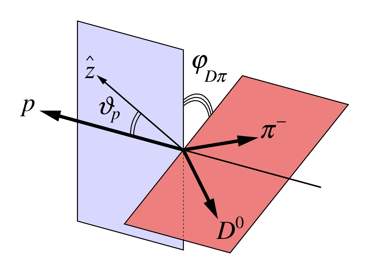 Figure 2
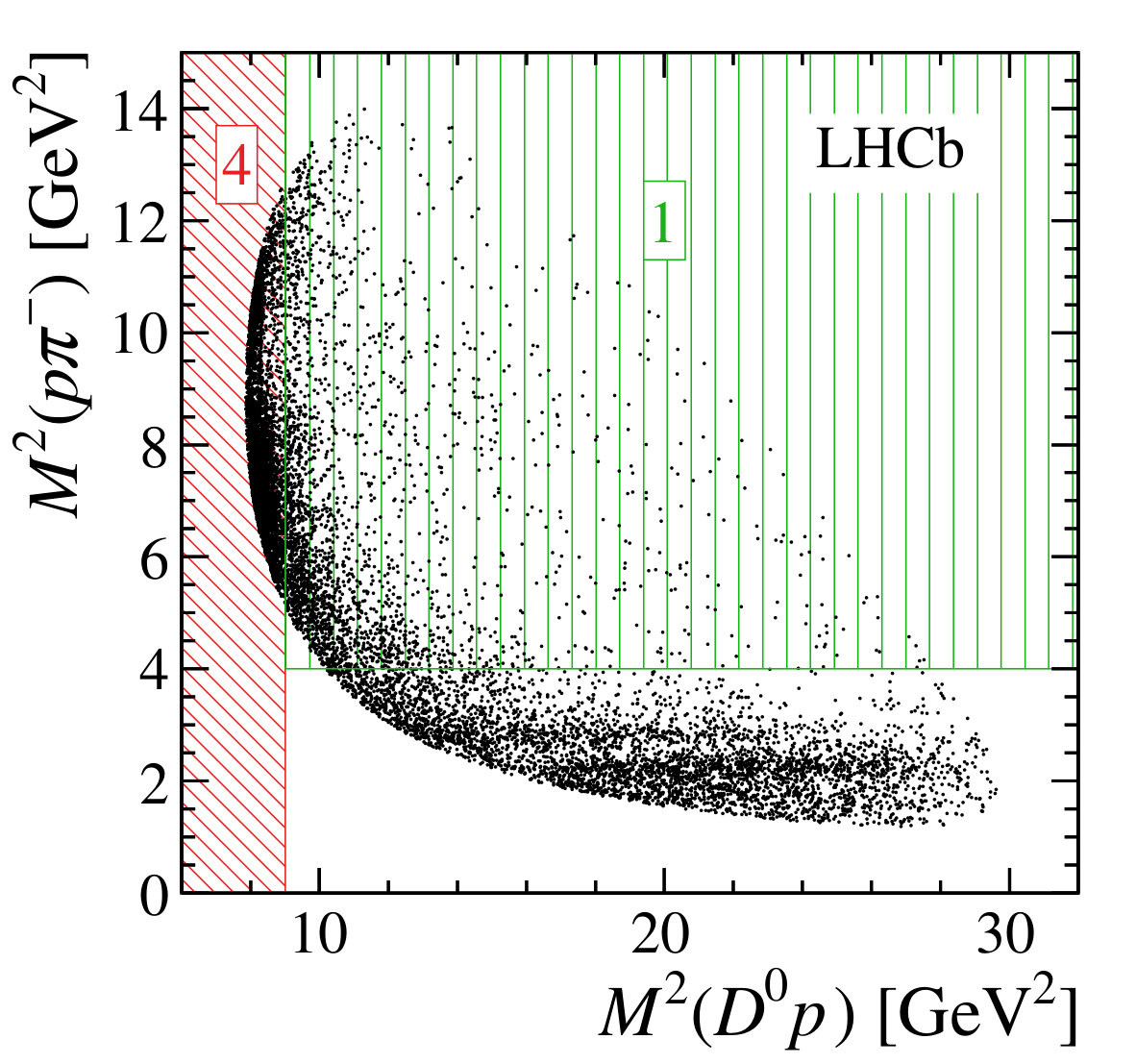 Figure 3
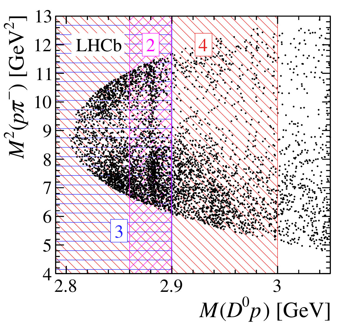 Figure 3
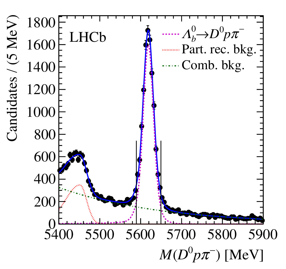 Figure 4
 Figure 5
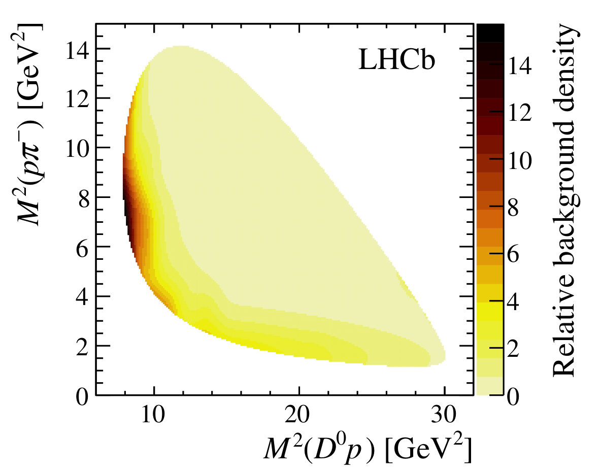 Figure 5
 Figure 6
 Figure 6
 Figure 6
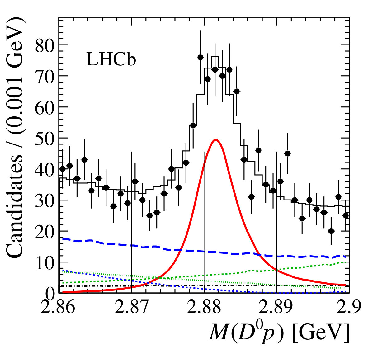 Figure 7
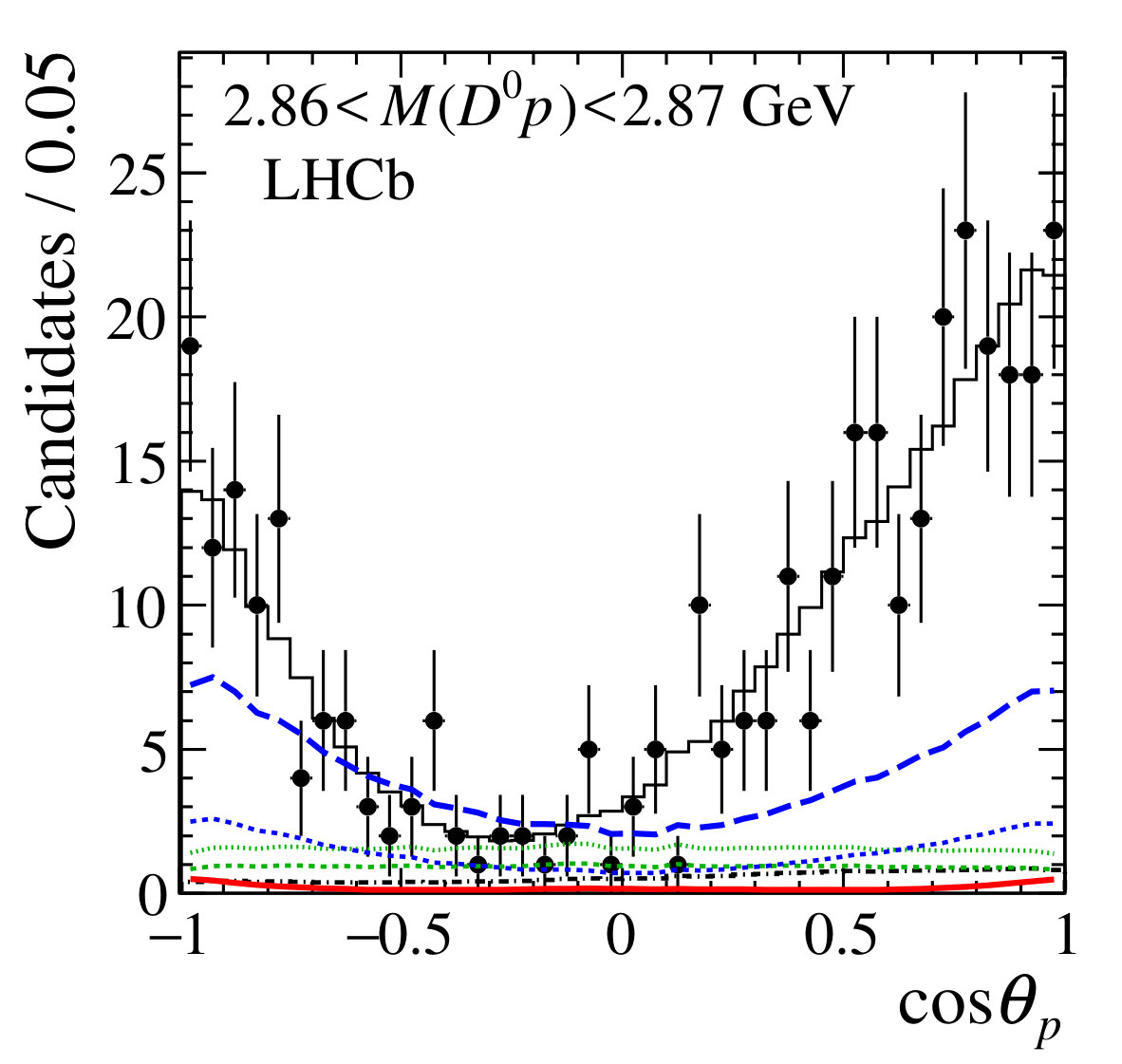 Figure 7
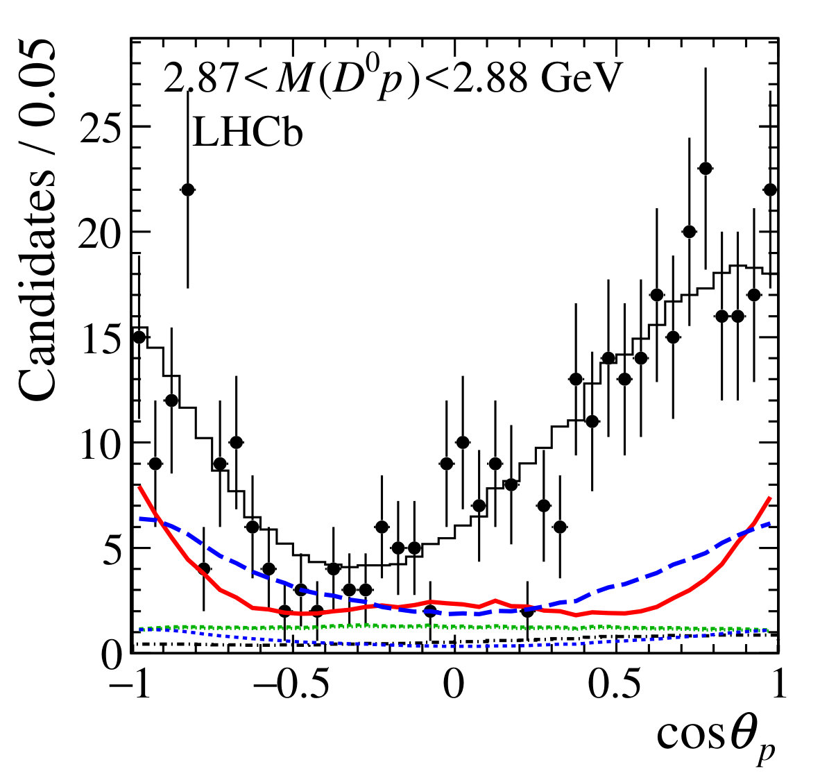 Figure 7
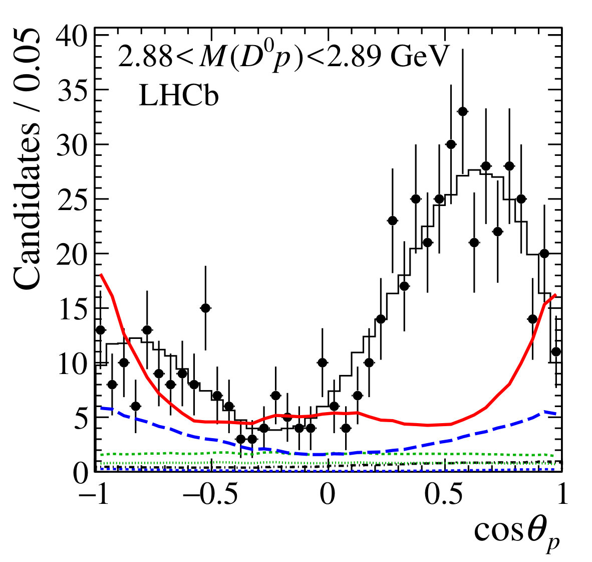 Figure 7
| Phase space region | |||||
| Yield | Full | 1 | 2 | 3 | 4 |
| Combinatorial | |||||
| Partially rec. | |||||
| Signal in box | 10 233 | 2 061 | 1 500 | 2 803 | 4 261 |
| Background in box | 1 616 | 598 | 89 | 192 | 427 |
| Region | Signal yield | yield |
|---|---|---|
| 2 | 09 | |
| 3 | 16 | |
| 4 | 61 |
| Uncertainty | |||
| Source | |||
| Background fraction | |||
| Efficiency profile | |||
| Background shape | |||
| Momentum resolution | |||
| Mass scale | |||
| Fit procedure | |||
| Total systematic | |||
| Breit–Wigner model | / | / | |
| Nonresonant model | / | / | |
| — of which helicity formalism | / | / | |
| Total model | / | / | |
| Nonresonant model | Resonance | |||||||
| Mass | ndf | [%] | ||||||
| Exp | Exp | Exp | Exp | 287.4/150 | 00.0 | |||
| Exp | Exp | Exp | Exp | 2765 | 247.2/146 | 00.0 | ||
| Exp | Exp | Exp | Exp | 2765 | 254.8/146 | 00.0 | ||
| Exp | Exp | Exp | Exp | 2765 | 240.5/146 | 00.0 | ||
| Exp | Exp | Exp | Exp | 2765 | 226.0/146 | 00.0 | ||
| Exp | Exp | Exp | Exp | Float | 162.7/145 | 14.9 | ||
| Exp | Exp | Exp | Exp | Float | 170.2/145 | 07.5 | ||
| Exp | Exp | Exp | Exp | Float | 162.1/145 | 15.7 | ||
| Exp | Exp | Exp | Exp | Float | 139.5/145 | 61.3 | ||
| Exp | Exp | Float | 169.7/153 | 16.9 | ||||
| Exp | Exp | Exp | Float | 0.0 | 62.1 | |||
| CSpl | Exp | Exp | Exp | 181.3/140 | 01.1 | |||
| Exp | CSpl | Exp | Exp | 154.8/140 | 18.5 | |||
| Exp | Exp | CSpl | Exp | 172.9/140 | 03.1 | |||
| Exp | Exp | Exp | CSpl | 146.6/140 | 33.4 | |||
| Exp | Exp | CSpl | 234.8/143 | 00.0 | ||||
| Exp | Exp | CSpl | 165.7/143 | 09.4 | ||||
| Exp | Exp | CSpl | CSpl | 146.1/130 | 15.8 | |||
| Exp | Exp | RSpl | Exp | 177.0/143 | 02.8 | |||
| Exp | Exp | Exp | RSpl | 174.5/143 | 03.8 | |||
| Exp | Exp | RSpl | RSpl | 145.1/138 | 32.3 | |||
|
|
|
|
|
|
|
|
|
|---|---|---|---|---|---|---|---|
| Uncertainty | |||||
| Source | |||||
| [%] | [%] | [%] | |||
| Background fraction | |||||
| Efficiency profile | |||||
| Background shape | |||||
| Momentum resolution | |||||
| Mass scale | |||||
| Fit procedure | |||||
| parameters | |||||
| Total systematic | |||||
| Breit–Wigner model | / | /1 | / | / | / |
| Nonresonant model | / | /1 | / | / | / |
| — of which hel. form. | / | /1 | / | / | / |
| / | /1 | / | / | / | |
| Total model | / | / | / | / | / |
Peer Reviews
No public reviews on file for this paper yet. If you reviewed it on a platform where reviews are public (OpenReview, ICLR, NeurIPS, ICML), you can paste yours below so the community can read it here.
Videos
No videos yet. Explain this paper in a talk, walkthrough, or lecture? Add one.
EUROPEAN ORGANIZATION FOR NUCLEAR RESEARCH (CERN)
CERN-EP-2017-007
LHCb-PAPER-2016-061
26 January 2017
Study of the amplitude in decays
The LHCb collaboration†††Authors are listed at the end of this paper.
An amplitude analysis of the decay is performed in the part of the phase space containing resonances in the channel. The study is based on a data sample corresponding to an integrated luminosity of 3.0 of collisions recorded by the LHCb experiment. The spectrum of excited states that decay into is studied. The masses, widths and quantum numbers of the and resonances are measured. The constraints on the spin and parity for the state are obtained for the first time. A near-threshold enhancement in the amplitude is investigated and found to be consistent with a new resonance, denoted the , of spin and positive parity.
Submitted to JHEP
© CERN on behalf of the LHCb collaboration, licence CC-BY-4.0.
1 Introduction
Decays of beauty baryons to purely hadronic final states provide a wealth of information about the interactions between the fundamental constituents of matter. Studies of direct violation in these decays can help constrain the parameters of the Standard Model and New Physics effects in a similar way as in decays of beauty mesons [1, 2, 3, 4, 5, 6, 7]. Studies of the decay dynamics of beauty baryons can provide important information on the spectroscopy of charmed baryons, since the known initial state provides strong constraints on the quantum numbers of intermediate resonances. The recent observation of pentaquark states at LHCb [8] has renewed the interest in baryon spectroscopy.
The present analysis concerns the decay amplitude of the Cabibbo-favoured decay (the inclusion of charge-conjugate processes is implied throughout this paper). A measurement of the branching fraction of this decay with respect to the mode was reported by the LHCb collaboration using a data sample corresponding to of integrated luminosity [9]. The decay includes resonant contributions in the channel that are associated with intermediate excited states, as well as contributions in the channel due to excited nucleon () states. The study of the part of the amplitude will help to constrain the dynamics of the Cabibbo-suppressed decay , which is potentially sensitive to the angle of the Cabibbo-Kobayashi-Maskawa quark mixing matrix [10, 11]. The analysis of the amplitude is interesting in its own right. One of the states decaying to , the , has a possible interpretation as a molecule [12, 13, 14, 15, 16, 17, 18, 19, 20]. There are currently no experimental constraints on the quantum numbers of the state.
The mass spectrum of the predicted and observed orbitally excited states [21] is shown in Fig. 1. In addition to the ground state and to the and states, which are identified as the members of the -wave doublet, a -wave doublet with higher mass is predicted. One of the members of this doublet could be the state known as the , which is measured to have spin and parity [22, 23], while no candidate for the other state has been observed yet. Several theoretical studies provide mass predictions for this state and other excited charm baryons [24, 25, 26, 21, 27, 28, 29]. The BaBar collaboration has previously reported indications of a structure in the mass spectrum close to threshold, at a mass around 111Natural units with are used throughout., which could be the missing member of the -wave doublet [30].
This analysis is based on a data sample corresponding to an integrated luminosity of 3.0 of collisions recorded by the LHCb detector, with 1.0 collected at centre-of-mass energy in 2011 and 2.0 at in 2012.
The paper is organised as follows. Section 2 gives a brief description of the LHCb experiment and its reconstruction and simulation software. The amplitude analysis formalism and fitting technique is introduced in Sec. 3. The selection of candidates is described in Sec. 4, followed by the measurement of signal and background yields (Sec. 5), evaluation of the efficiency (Sec. 6), determination of the shape of the background distribution (Sec. 7), and discussion of the effects of momentum resolution (Sec. 8). Results of the amplitude fit are presented in Sec. 9 separately for four different regions of the phase space, along with the systematic uncertainties for those fits. Section 10 gives a summary of the results.
2 Detector and simulation
The LHCb detector [31, 32] is a single-arm forward spectrometer covering the pseudorapidity range , designed for the study of particles containing or quarks. The detector includes a high-precision tracking system consisting of a silicon-strip vertex detector surrounding the interaction region, a large-area silicon-strip detector located upstream of a dipole magnet with a bending power of about , and three stations of silicon-strip detectors and straw drift tubes placed downstream of the magnet. The tracking system provides a measurement of momentum, , of charged particles with relative uncertainty that varies from 0.5% at low momentum to 1.0% at 200. The minimum distance of a track to a primary vertex (PV), the impact parameter (IP), is measured with a resolution of (15+29/\mbox{p_{\mathrm{T}}}){\,\upmu\mathrm{m}}, where is the component of the momentum transverse to the beam, in . Different types of charged hadrons are distinguished using information from two ring-imaging Cherenkov detectors. Photons, electrons and hadrons are identified by a calorimeter system consisting of scintillating-pad and preshower detectors, an electromagnetic calorimeter and a hadronic calorimeter. Muons are identified by a system composed of alternating layers of iron and multiwire proportional chambers.
The online event selection is performed by a trigger [33], which consists of a hardware stage, based on information from the calorimeter and muon systems, followed by a software stage, which applies a full event reconstruction. At the hardware trigger stage, events are required to have a muon with high or a hadron, photon or electron with high transverse energy in the calorimeters. The software trigger requires a two-, three- or four-track secondary vertex with significant displacement from any PV in the event. At least one charged particle forming the vertex must exceed a threshold in the range 1.6–1.7 and be inconsistent with originating from a PV. A multivariate algorithm [34] is used for the identification of secondary vertices consistent with the decay of a hadron.
In the simulation, collisions are generated using Pythia 8 [35, *Sjostrand:2007gs] with a specific LHCb configuration [37]. Decays of hadronic particles are described by EvtGen [38], in which final-state radiation is generated using Photos [39]. The interaction of the generated particles with the detector, and its response, are implemented using the Geant4 toolkit [40, *Agostinelli:2002hh] as described in Ref. [42].
3 Amplitude analysis formalism
The amplitude analysis is based on the helicity formalism used in previous LHCb analyses. A detailed description of the formalism can be found in Refs. [43, 44, 8]. This section gives details of the implementation specific to the decay .
3.1 Phase space of the decay
Three-body decays of scalar particles are described by the two-dimensional phase space of independent kinematic parameters, often represented as a Dalitz plot [45]. For baryon decays, in general also the additional angular dependence of the decay products on the polarisation of the decaying particle has to be considered.
A vector of five kinematic variables (denoted ) describes the phase space of the decay . The kinematic variables are the two Dalitz plot variables, namely the invariant masses squared of the and combinations and , and three angles that determine the orientation of the three-body decay plane (Fig. 2). These angles are defined in the rest frame of the decaying baryon with the axis given by the direction of the baryon in the laboratory frame, the polarisation axis given by the cross-product of beam direction and axis, and the axis given by the cross-product of the and axes. The angular variables are the cosine of the polar angle , and the azimuthal angle of the proton momentum in the reference frame defined above (Fig. 2(a)), and the angle between the plane and the plane formed by the proton direction and the polarisation axis (Fig. 2(b)).
3.2 Helicity formalism
The baseline amplitude fit uses the helicity formalism where the interfering amplitude components are expressed as sequential quasi-two-body decays , (where denotes the intermediate resonant or nonresonant state). The decay amplitude for a baryon with spin projection decaying via an intermediate state with helicity into a final state with proton helicity is
[TABLE]
where and are the spins of the baryon and the state, are the reduced Wigner functions, and and are complex constants (couplings). The mass-dependent complex lineshape defines the dynamics of the decay. The angles defining the helicity amplitude are the polar () and azimuthal () angles of the intermediate state in the reference frame defined above, and the polar () and azimuthal () angles of the final-state proton in the frame where the intermediate state is at rest and the polar axis points in the direction of in the rest frame. All of these angles are functions of the five phase space variables defined previously and thus do not constitute additional degrees of freedom.
The strong decay conserves parity, which implies that
[TABLE]
where , and are the spins of the proton, meson and resonance , respectively, and , and are their parities. This relation reduces the number of free parameters in the helicity amplitudes: is absorbed by , and each coefficient enters the amplitude multiplied by a factor . The convention used is
[TABLE]
As a result, only two couplings remain for each intermediate state , corresponding to its two allowed helicity configurations. The two couplings are denoted for brevity as .
The amplitude, for fixed and , after summation over the intermediate resonances and their two possible helicities is
[TABLE]
To obtain the decay probability density, the amplitudes corresponding to different polarisations of the initial- and final-state particles have to be summed up incoherently. The baryons produced in collisions can only have polarisation transverse to the production plane, i.e. along the axis. The longitudinal component is forbidden due to parity conservation in the strong processes that dominate production. In this case, the probability density function (PDF) of the kinematic variables that characterise the decay of a with the transverse polarisation , after summation over and , is proportional to
[TABLE]
Equations (4) and (5) can be combined to yield the simplified expression:
[TABLE]
where is the highest spin among the intermediate resonances and and are functions of only . As a consequence, does not depend on the azimuthal angles and . Dependence on the angle appears only if the is polarised. In the unpolarised case the density depends only on the internal degrees of freedom and (which in turn can be expressed as a function of the other Dalitz plot variable, ). Moreover, after integration over the angle , the dependence on polarisation cancels if the detection efficiency is symmetric over . Since polarisation in collisions is measured to be small (, [46]) and the efficiency is highly symmetric in , the effects of polarisation can safely be neglected in the amplitude analysis, and only the Dalitz plot variables need to be used to describe the probability density of the decay. The density is given by Eq. (5) with such that no dependence on the angles , or remains.
Up to this point, the formalism has assumed that resonances are present only in the channel. While in the case of decays the regions of phase space with contributions from and resonances are generally well separated, there is a small region where they can overlap, and thus interference between resonances in the two channels has to be taken into account. In the helicity formalism, the proton spin-quantisation axes are different for the helicity amplitudes corresponding to and resonances [8]: they are parallel to the proton direction in the and rest frames, and are thus antiparallel to the and momenta, respectively. The rotation angle between the two spin-quantisation axes is given by
[TABLE]
where and are the momenta of the and mesons, respectively, in the proton rest frame.
If the proton spin-quantisation axis is chosen with respect to the resonances and the helicity basis is denoted as , the helicity states corresponding to states are
[TABLE]
and thus the additional terms in the amplitude (Eq. (4)) related to the channel are expressed as
[TABLE]
where the angles , , and are defined in a similar way as , , and , but with the intermediate state in the channel.
3.3 Resonant and nonresonant lineshapes
The part of the amplitude that describes the dynamics of the quasi-two-body decay, , is given by one of the following functions. Resonances are parametrised with relativistic Breit–Wigner lineshapes multiplied by angular barrier terms and corrected by Blatt–Weisskopf form factors [47]:
[TABLE]
with mass-dependent width given by
[TABLE]
where and are the pole parameters of the resonance. The Blatt–Weisskopf form factors for the resonance, , and for the , , are parametrised as
[TABLE]
where the definitions of the terms and depend on whether the form factor for the resonance or for the is being considered. For these terms are given by and , where is the centre-of-mass momentum of the decay products in the two-body decay with the mass of the resonance equal to , , and is a radial parameter taken to be . For the respective functions are and , where is the centre-of-mass momentum of decay products in the two-body decay , , and . The analysis is very weakly sensitive to the values of , and these are varied in a wide range for assessing the associated systematic uncertainty (Sec. 9.2).
The mass-dependent width and form factors depend on the orbital angular momenta of the two-body decays. For the weak decay of the , the minimum possible angular momentum (where is the spin of the resonance) is taken, while for the strong decay of the intermediate resonance, the angular momentum is fully determined by the parity of the resonance, , and conservation of angular momentum, which requires .
Two parametrisations are used for nonresonant amplitudes: exponential and polynomial functions. The exponential nonresonant lineshape [48] used is
[TABLE]
where is a shape parameter. The polynomial nonresonant lineshape [49] used is
[TABLE]
where , and is a constant that is chosen to minimise the correlations between the coefficients when they are treated as free parameters. In the case of the amplitude fit, is chosen to be near the middle of the fit range, . In both the exponential and the polynomial parametrisations, also serves as the resonance mass parameter in the definition of and in the angular barrier terms. Note that in Ref. [49] the polynomial form was introduced to describe the slow variations of a nonresonant amplitude across the large phase space of charmless decays, and thus the parameters were defined as complex constants to allow slow phase motion over the wide range of invariant masses. In the present analysis, the phase space is much more constrained and no significant phase rotation is expected for the nonresonant amplitudes. The coefficients thus are taken to be real.
To study the resonant nature of the states, model-independent parametrisations of the lineshape are used. One approach used here consists of interpolation with cubic splines, done independently for the real and imaginary parts of the amplitude (referred to as the “complex spline” lineshape) [50]. The free parameters of such a fit are the real and imaginary parts of the amplitude at the spline knot positions. Alternatively, to assess the significance of the complex phase rotation in a model-independent way, a spline-interpolated shape is used in which the imaginary parts of the amplitude at all knots are fixed to zero (“real spline”).
3.4 Fitting procedure
An unbinned maximum likelihood fit is performed in the two-dimensional phase space . Defining as the likelihood function, the fit minimises
[TABLE]
where the summation is performed over all candidates in the data sample and is the normalised PDF. It is given by
[TABLE]
where is the signal PDF, is the background PDF, is the efficiency, and and are the signal and background normalisations:
[TABLE]
and
[TABLE]
where the integrals are taken over the part of the phase space used in the fit (Section 5), and and are the numbers of signal and background events in the signal region, respectively, evaluated from a fit to the invariant mass distribution. The normalisation integrals are calculated numerically using a fine grid with cells in the baseline fits; the numerical uncertainty is negligible compared with the other uncertainties in the analysis.
3.5 Fit parameters and fit fractions
The free parameters in the fit are the couplings for each of the amplitude components and certain parameters of the lineshapes (such as the masses and/or widths of the resonant states, or shape parameters of the nonresonant lineshapes). Since the overall normalisation of the density is arbitrary, one of the couplings can be set to unity. In this analysis, the convention for the state is used. Additionally, the amplitudes corresponding to different helicity states of the initial- and final-state particles are added incoherently, so that the relative phase between and for one of the contributions is arbitrary. The convention for the is used.
The definitions of the polynomial and spline-interpolated shapes already contain terms that characterise the relative magnitudes of the corresponding amplitudes. The couplings for them are defined in such a way as to remove the additional degree of freedom from the fit. For the polynomial and real spline lineshapes, the following couplings are used:
[TABLE]
where , and are free parameters. For the complex spline lineshape, a similar parametrisation is used with fixed to zero, since the complex phase is already included in the spline definition.
The observable decay density for an unpolarised particle in the initial state does not allow each polarisation amplitude to be obtained independently. As a result, the couplings in the fit can be strongly correlated. However, the size of each contribution can be characterised by its spin-averaged fit fraction
[TABLE]
If all the components correspond to partial waves with different spin-parities, the sum of the spin-averaged fit fractions will be 100%; otherwise it can differ from 100% due to interference effects. The statistical uncertainties on the fit fractions are obtained from ensembles of pseudoexperiments.
3.6 Evaluation of fit quality
To assess the goodness of each fit, a value is calculated by summing over the bins of the two-dimensional Dalitz plot. Since the amplitude is highly non-uniform and a meaningful test requires a certain minimum number of entries in each bin, an adaptive binning method is used to ensure that each bin contains at least 20 entries in the data.
Since the fit itself is unbinned, some information is lost by the binning. The number of degrees of freedom for the test in such a case is not well defined. The effective number of degrees of freedom () should be in the range , where is the number of bins and is the number of free parameters in the fit. For each fit, is obtained from ensembles of pseudoexperiments by requiring that the probability value for the distribution with degrees of freedom, , is distributed uniformly.
Note that when two fits with different models have similar binned values, it does not necessarily follow that both models describe the data equally well. Since the bins in regions with low population density have large area, the binning can obscure features that could discriminate between the models. This information is preserved in the unbinned likelihood. Thus, discrimination between fit models is based on the difference , the statistical significance of which is determined using ensembles of pseudoexperiments. The binned serves as a measure of the fit quality for individual models and is not used to discriminate between them.
4 Signal selection
The analysis uses the decay , where mesons are reconstructed in the final state . The selection of candidates is performed in three stages: a preliminary selection, a kinematic fit, and a final selection. The preliminary selection uses loose criteria on the kinematic and topological properties of the candidate. All tracks forming a candidate, as well as the and vertices, are required to be of good quality and be separated from every PV in the event. The separation from a PV is characterised by a quantity , defined as the increase in the vertex-fit when the track (or combination of tracks corresponding to a short-lived particle) is included into the vertex fit. The tracks forming a candidate are required to be positively identified as a pion and a kaon, and the and decay vertices are required to be downstream of their production vertices. All of the tracks are required to have no associated hits in the muon detector.
For candidates passing this initial selection, a kinematic fit is performed [51]. Constraints are imposed that the and decay products originate from the corresponding vertices, that the candidate originate from its associated PV (the one with the smallest value of for the ), and that the mass of the candidate be equal to its known value [23]. The kinematic fit is required to converge with a good , and the mass of the candidate after the fit is required to be in the range –. To suppress background from charmless decays, the decay time significance of the candidate obtained after the fit is required to be greater than one standard deviation. To improve the resolution of the squared invariant masses and entering the amplitude fit, the additional constraint that the invariant mass of the combination be equal to the known mass [23] is applied when calculating these variables.
After the initial selection, the background in the region of the signal is dominated by random combinations of tracks. The final selection is based on a boosted decision tree (BDT) algorithm [52, 53] designed to separate signal from this background. The selection is trained using simulated events generated uniformly across the phase space as the signal sample, and the sample of opposite-flavour , combinations from data as background. In total, 12 discriminating variables are used in the BDT selection: the of the kinematic fit, the angle between the momentum and the direction of flight of the candidate, the of the and vertex fits, the lifetime significance of the candidate with respect to the vertex, the of the final-state tracks and the candidate, and the particle identification (PID) information of the proton and pion tracks from the vertex. Due to differences between simulation and data, corrections are applied to all the variables from the simulated sample used in the BDT training, except for the PID variables. These corrections are typically about and are obtained from a large and clean sample of decays. The simulated proton and pion PID variables are replaced with values generated using distributions obtained from calibration samples of and decays in data. For these calibration samples, the four-dimensional distributions of PID variable, , and the track multiplicity of the event are described using a nonparametric kernel-based procedure [54]. The resulting distributions are used to generate PID variables for each pion or proton track given its , and the track multiplicity in the simulated event.
The BDT requirement is chosen such that the fraction of background in the signal region used for the subsequent amplitude fit, , does not exceed 15%. This corresponds to a signal efficiency of 66% and a background rejection of 96% with respect to the preliminary selection. After all selection requirements are applied, fewer than 1% of selected events contain a second candidate. All multiple candidates are retained; the associated systematic uncertainty is negligible.
5 Fit regions and event yields
The Dalitz plot of selected events, without background subtraction or efficiency correction, in the signal invariant mass range defined in Sec. 4 is shown in Fig. 3(a). The part of the phase space near the threshold that contains contributions from resonances is shown in Fig. 3(b). The latter uses as the horizontal axis instead of .
In Fig. 3, the four amplitude fit regions of the phase space are indicated. These are denoted regions 1–4. Region 1, and , is the part of the phase space that does not include resonant contributions and is used only to constrain the nonresonant amplitude in the regions. Region 2, , contains the well-known state and is used to measure its parameters and to constrain the slowly varying amplitude underneath it in a model-independent way. The fit in region 3 near the threshold, , provides additional information about the slowly-varying amplitude. Finally, the fit in region 4, , which includes the state, gives information about the properties of this resonance and the relative magnitudes of the resonant and nonresonant contributions. Note that region 2 is fully contained in region 3, while region 3 is fully contained in region 4.
The signal and background yields in each region are obtained from extended unbinned maximum likelihood fits of the invariant mass distribution in the range –. The fit model includes the signal component, a contribution from random combinations of tracks (combinatorial background) and the background from partially reconstructed decays (where decays into or and the or are not included in the reconstruction).
The signal component is modelled as the sum of two Crystal Ball functions [55] with the same most probable value and power-law tails on both sides. All parameters of the model are fixed from simulation except for the peak position and a common scale factor for the core widths, which are floated in the fit to data. The combinatorial background is parametrised by an exponential function, and the partially reconstructed background is described by a bifurcated Gaussian distribution. The shape parameters of the background distributions are free parameters of the fit.
The results of the fit for candidates in the entire phase space are shown in Fig. 4. The background and signal yields in the entire phase space, as well as in the regions used in the amplitude fit, are given in Table 5.
The reference list from the paper itself. Each links out to its DOI / PubMed record.
- 1[1] I. Dunietz, CP violation with beautiful baryons , Z. Phys. C 56 (1992) 129 · doi ↗
- 2[2] Fayyazuddin, Λ b 0 → Λ + D 0 ( D ¯ ) 0 {{\mathchar 28931\relax}^{0}_{b}}\rightarrow{\mathchar 28931\relax}+{{D}^{0}}({{\kern 1.99997 pt\overline{\kern-1.99997 pt D}{}}{}^{0}}) decays and CP-violation , Mod. Phys. Lett. A 14 (1999) 63 , ar Xiv:hep-ph/9806393 · doi ↗
- 3[3] A. K. Giri, R. Mohanta, and M. P. Khanna, Possibility of extracting the weak phase γ 𝛾 \gamma from Λ b 0 → Λ D 0 → subscript superscript Λ 0 𝑏 Λ superscript 𝐷 0 {{\mathchar 28931\relax}^{0}_{b}}\rightarrow{\mathchar 28931\relax}D^{0} decays , Phys. Rev. D 65 (2002) 073029 , ar Xiv:hep-ph/0112220 · doi ↗
- 4[4] Y. K. Hsiao and C. Q. Geng, Direct CP violation in Λ b subscript Λ 𝑏 {\mathchar 28931\relax}_{b} decays , Phys. Rev. D 91 (2015) 116007 , ar Xiv:1412.1899 · doi ↗
- 5[5] W. Bensalem and D. London, T 𝑇 T -violating triple-product correlations in hadronic b 𝑏 b decays , Phys. Rev. D 64 (2001) 116003 , ar Xiv:hep-ph/0005018 · doi ↗
- 6[6] W. Bensalem, A. Datta, and D. London, New-physics effects on triple-product correlations in Λ b 0 subscript superscript Λ 0 𝑏 {\mathchar 28931\relax}^{0}_{b} decays , Phys. Rev. D 66 (2002) 094004 , ar Xiv:hep-ph/0208054 · doi ↗
- 7[7] W. Bensalem, A. Datta, and D. London, T-violating triple-product correlations in charmless Λ b 0 subscript superscript Λ 0 𝑏 {\mathchar 28931\relax}^{0}_{b} decays , Phys. Lett. B 538 (2002) 309 , ar Xiv:hep-ph/0205009 · doi ↗
- 8[8] LH Cb collaboration, R. Aaij et al. , Observation of J / ψ p 𝐽 𝜓 𝑝 {{J\mskip-3.0mu/\mskip-2.0mu\psi\mskip 2.0mu}}{p} resonances consistent with pentaquark states in Λ b 0 → J / ψ p K − → subscript superscript Λ 0 𝑏 𝐽 𝜓 𝑝 superscript 𝐾 {{\mathchar 28931\relax}^{0}_{b}}\rightarrow{{J\mskip-3.0mu/\mskip-2.0mu\psi\mskip 2.0mu}}{p}{{K}^{-}} decays , Phys. Rev. Lett. 115 (2015) 072001 , ar Xiv:1507.03414 · doi ↗