This paper introduces an adaptive isogeometric finite element method using hierarchical B-splines for elliptic PDEs, achieving optimal convergence rates through a novel refinement strategy guided by an a posteriori error estimator.
Contribution
It develops a new adaptive algorithm for IGAFEM with hierarchical B-splines, proving optimal convergence rates and supporting findings with numerical experiments.
Findings
01
Linear convergence of the error estimator
02
Optimal algebraic convergence rates achieved
03
Numerical experiments confirm theoretical results
Abstract
We consider an adaptive algorithm for finite element methods for the isogeometric analysis (IGAFEM) of elliptic (possibly non-symmetric) second-order partial differential equations in arbitrary space dimension d≥2. We employ hierarchical B-splines of arbitrary degree and different order of smoothness. We propose a refinement strategy to generate a sequence of locally refined meshes and corresponding discrete solutions. Adaptivity is driven by some weighted residual a posteriori error estimator. We prove linear convergence of the error estimator (resp. the sum of energy error plus data oscillations) with optimal algebraic rates. Numerical experiments underpin the theoretical findings.
\displaystyle\langle w\,,\,v\rangle_{\mathcal{L}}\leq\big{(}\|\textit{{A}}\|_{L^{\infty}(\Omega)}+\|\textit{{b}}\|_{L^{\infty}(\Omega)}+\|c\|_{L^{\infty}(\Omega)}\big{)}\|w\|_{H^{1}(\Omega)}\|v\|_{H^{1}(\Omega)}\text{ for all $v,w\in H^{1}(\Omega)$.}
\displaystyle\langle w\,,\,v\rangle_{\mathcal{L}}\leq\big{(}\|\textit{{A}}\|_{L^{\infty}(\Omega)}+\|\textit{{b}}\|_{L^{\infty}(\Omega)}+\|c\|_{L^{\infty}(\Omega)}\big{)}\|w\|_{H^{1}(\Omega)}\|v\|_{H^{1}(\Omega)}\text{ for all $v,w\in H^{1}(\Omega)$.}
\displaystyle\mathbb{T}(N):=\big{\{}{\mathcal{T}}_{\bullet}\in\mathbb{T}\,:\,\#{\mathcal{T}}_{\bullet}-\#{\mathcal{T}}_{0}\leq N\big{\}}\quad\text{for all }N\in{\mathbb{N}}_{0}
\displaystyle\mathbb{T}(N):=\big{\{}{\mathcal{T}}_{\bullet}\in\mathbb{T}\,:\,\#{\mathcal{T}}_{\bullet}-\#{\mathcal{T}}_{0}\leq N\big{\}}\quad\text{for all }N\in{\mathbb{N}}_{0}
No public reviews on file for this paper yet. If you reviewed it on a platform where reviews are public (OpenReview, ICLR, NeurIPS, ICML), you can paste yours below so the community can read it here.
Videos
No videos yet. Explain this paper in a talk, walkthrough, or lecture? Add one.
Full text
Adaptive IGAFEM with optimal convergence rates:
Hierarchical B-splines
Gregor Gantner
,
Daniel Haberlik
and
Dirk Praetorius
Abstract.
We consider an adaptive algorithm for finite element methods for the isogeometric analysis (IGAFEM) of elliptic (possibly non-symmetric) second-order partial differential equations in arbitrary space dimension d≥2. We employ hierarchical B-splines of arbitrary degree and different order of smoothness.
We propose a refinement strategy to generate a sequence of locally refined meshes and corresponding discrete solutions.
Adaptivity is driven by some weighted residual a posteriori error estimator.
We prove linear convergence of the error estimator
(resp. the sum of energy error plus data oscillations)
with optimal algebraic rates. Numerical experiments underpin the theoretical findings.
The central idea of isogeometric analysis (IGA) is to use the same ansatz functions for the discretization of the partial differential equation (PDE) as for the representation of the problem geometry in computer aided design (CAD); see [HCB05, CHB09, BBdVC*+*06].
The CAD standard for spline representation in a multivariate setting relies on tensor-product B-splines.
However, to allow for adaptive refinement, several extensions of the B-spline model have recently emerged, e.g., analysis-suitable T-splines [SLSH12, BdVBSV13], hierarchical splines [VGJS11, GJS12, KVVdZvB14], or LR-splines [DLP13, JKD14]; see also [JRK15, HKMP16] for a comparison of these approaches.
All these concepts have been studied via numerical experiments.
However, so far there exists only little literature concerning the thorough mathematical analysis of adaptive isogeometric finite element methods (IGAFEM).
Indeed, we are only aware of the works [BG16a] which investigates an estimator reduction of an IGAFEM with certain hierarchical splines introduced in [BG15], as well as [BG16b] which investigates linear convergence of an IGAFEM with truncated hierarchical B-splines introduced in [GJS12].
In the continuation of the latter work [BG16b], [BGMP16] studied the corresponding mesh-refinement strategy together with some refinement-related properties for the proof of optimal convergence.
However, the mathematical proof that the adaptive strategy of [BG16b] leads to optimal convergence rates, is still missing in the literature.
Moreover, in this case one cannot use hierarchical B-splines for the implementation, but has to use truncated hierarchical B-splines instead.
It is important to note that the procedure of truncation requires a specific construction that entails complicated supports of the basis functions, which are in general not even connected, and their use may produce an overhead with an adaptive strategy that cannot be neglected.
For standard FEM with globally continuous piecewise polynomials, adaptivity is well understood; see, e.g., [Dör96, MNS00, BDD04, Ste07, CKNS08, FFP14, CFPP14] for milestones on convergence and optimal convergence rates.
In the frame of isogeometric boundary element methods (IGABEM), we
also mention our recent work [FGHP16b] which shows linear convergence with optimal rates for some adaptive isogeometric boundary element method in 2D from [FGP15, FGHP16a],
where it is however sufficient to use the span of univariate non-uniform rational B-splines (NURBS).
1.2. Model problem
On the bounded Lipschitz-domain Ω⊂Rd with d≥2, we consider a general second-order linear elliptic PDE in divergence form with homogenous Dirichlet boundary conditions
[TABLE]
We pose the following regularity assumptions on the coefficients:
A(x)∈Rsymd×d is a symmetric matrix with A∈W1,∞(Ω).
The vector b(x)∈Rd and the scalar c(x)∈R satisfy b,c∈L∞(Ω).
We interpret L in its weak form and define the corresponding bilinear form
[TABLE]
The bilinear form is continuous, i.e., it holds that
[TABLE]
Additionally, we suppose ellipticity of ⟨⋅,⋅⟩L on H01(Ω), i.e.,
[TABLE]
Note that (1.4) is for instance satisfied if A(x) is uniformly positive definite and if b∈H(div,Ω) with −21divb(x)+c(x)≥0 almost everywhere in Ω.
Overall, the boundary value problem (1.1) fits into the setting of the Lax-Milgram theorem and therefore admits a unique solution u∈H01(Ω) to the weak formulation
[TABLE]
Finally, we note that the additional regularity A∈W1,∞(Ω) (instead of A∈L∞(Ω)) is only required for the well-posedness of the residual a posteriori error estimator, see Section 2.
1.3. Outline & Contributions
The remainder of this work is roughly organized as follows: Section 2 provides an abstract framework for adaptive mesh-refinement for conforming FEM for the model problem (1.1). Its main result is Theorem 2.4 which states optimal convergence behavior of some standard adaptive algorithm.
Section 3 considers conforming FEM based on hierarchical splines. Its main result is Theorem 3.8 which states that hierarchical splines fit into the framework of Section 2. The proofs of Theorem 2.4 and Theorem 3.8 are given in Section 4 and Section 5, respectively.
Three numerical experiments in Section 6 underpin the optimal convergence behavior of adaptive IGAFEM with hierarchical splines.
In more detail, the contribution of Section 2 can be paraphrased as follows: We formulate the standard adaptive strategy (Algorithm 2.3) driven by some residual a posteriori error estimator (2.9) in the frame of conforming FEM. We formulate three assumptions (M1)–(M3) for the underlying meshes (Section 2.1), five assumptions (R1)–(R5) on the mesh-refinement (Section 2.2), and six assumptions (S1)–(S6) on the
FEM spaces (Section 2.3).
First, these assumptions are sufficient to guarantee that the error estimator η∙ associated with the FEM solution U∙∈X∙⊂H01(Ω) is
efficient and
reliable, i.e., there exist
Ceff,
Crel>0 such that
[TABLE]
where osc∙(⋅) denotes certain data oscillation terms.
Second, Theorem 2.4 states that Algorithm 2.3 leads to linear convergence with optimal rates in the spirit of [CKNS08, CFPP14]: Let ηℓ denote the error estimator in the ℓ-th step of the adaptive algorithm. Then, there exist C>0 and 0<q<1 such that
[TABLE]
Moreover, for sufficiently small marking parameters in Algorithm 2.3, the estimator
(resp. the so-called total error ∥u−Uℓ∥H1(Ω)+oscℓ(Uℓ); see (1.6))
decays even with the optimal algebraic convergence rate in the sense of certain nonlinear approximation classes (Section 2.7).
In explicit terms, we identify sufficient conditions of the underlying meshes, the local FEM spaces, as well as the employed (local) mesh-refinement rule which guarantee that the related residual a posteriori error estimator satisfies the axioms of adaptivity from [CFPP14], so that
linear convergence with optimal rates for the standard adaptive algorithm follows.
While we exploit this framework only for IGAFEM with hierarchical splines, we believe that it might also serve as a promising starting point to analyze different technologies for adaptive IGAFEM like (analysis-suitable) T-splines or LR-splines, as well as for other conforming discretizations like the virtual element method (VEM) from [BdVBC*+*13].
Section 3 recalls the definition of hierarchical splines from [VGJS11], derives the canonical basis of the hierarchical spline space X∙⊂H01(Ω) with Dirichlet boundary conditions (Section 3.3), formulates an admissibility criterion (3.21) for hierarchical meshes (Section 3.4), and introduces some local mesh-refinement rule for admissible hierarchical meshes (Section 3.5).
One crucial observation is that the new mesh-refinement strategy for hierarchical meshes (Algorithm 3.5) guarantees that the number of (truncated) hierarchical B-splines on each element as well as the number of active elements contained in the support of each (truncated) hierarchical B-spline is uniformly bounded (Proposition 3.3). If one uses the strategy of [BG16b, BGMP16] instead, this property is is not satisfied for hierarchical B-splines, but only for truncated hierarchical B-splines. In general, the latter have a smaller, but also more complicated and not necessarily connected support.
The main result of Section 3 and the entire work is Theorem 3.8 which states that hierarchical splines together with the proposed local mesh-refinement strategy satisfy all assumptions of Section 2, so that Theorem 2.4 applies. In particular, our work goes beyond [BG16b] in two respects: While [BG16b] only proves linear convergence of the adaptive algorithm, we give the first proof of optimal convergence rates for IGAFEM. Moreover, [BG16b] adapts the analysis of [CKNS08] and is hence restricted to symmetric problems (i.e., b=0 and c≥0 in (1.1)). Our analysis exploits the framework of [CFPP14] together with some recent ideas from [FFP14, BHP17] and also covers the non-symmetric problem (1.1).
Technical contributions of general interest include the following: We prove that a hierarchical mesh is admissible if and only if it can be obtained by the mesh-refinement strategy of Algorithm 3.5 (Proposition 5.2). Moreover, admissible meshes also allow a simpler computation of truncated hierarchical B-splines in the sense that truncation simplifies considerably (Proposition 5.6). Together with some ideas from [SM16], we use this observation to define a Scott-Zhang-type projector J∙:L2(Ω)→X∙ which is locally L2- and H1-stable and has a first-order approximation property (Section 5.10).
1.4. General notation
Throughout, ∣⋅∣ denotes the absolute value of scalars, the Euclidean norm of vectors in Rd, as well as the d-dimensional measure of a set in Rd.
Moreover, # denotes the cardinality of a set as well as the multiplicity of a knot within a given knot vector.
We write A≲B to abbreviate A≤cB with some generic constant c>0 which is clear from the context. Moreover, A≃B abbreviates A≲B≲A. Throughout, mesh-related quantities have the same index, e.g., X∙ is the ansatz space corresponding to the mesh T∙.
The analogous notation is used for meshes T∘, T⋆ or Tℓ etc.
Moreover, we use ⋅ to transfer quantities in the physical domain Ω to the parameter domain Ω, e.g., we write T for the set of all admissible meshes in the parameter domain instead of T which denotes the set of all admissible meshes in the physical domain.
2. Axioms of adaptivity (revisited)
The aim of this section is to formulate an adaptive algorithm (Algorithm 2.3) for conforming FEM discretizations of our model problem (1.1), where adaptivity is driven by the residual a posteriori error estimator (see (2.9) below).
We identify the crucial properties of the underlying meshes, the mesh-refinement, as well as the finite element spaces which ensure that the residual error estimator fits into the general framework of [CFPP14] and which hence guarantee optimal convergence behavior of the adaptive algorithm.
The main result of this section is Theorem 2.4 which is proved in Section 4.
2.1. Meshes
Throughout, T∙ is a mesh of Ω in the following sense:
•
T∙ is a finite set of compact Lipschitz domains;
•
for all T,T′∈T∙ with T=T′, the intersection T∩T′ has measure zero;
•
Ω=⋃T∈T∙T, i.e., T∙ is a partition of Ω.
We suppose that there is a countably infinite set T of admissible meshes. For T∙∈T and ω⊆Ω, we define the patches of order k∈N0 inductively by
[TABLE]
The corresponding set of elements is
[TABLE]
To abbreviate notation, we let π∙(ω):=π∙1(ω) and Π∙(ω):=Π∙1(ω).
For \SS∙⊆T∙, we define π∙k(\SS∙):=π∙k(⋃\SS∙)
and Π∙k(\SS∙):=Π∙k(⋃\SS∙).
We suppose that there exist Cshape,Cpatch,Ctrace>0 such that all meshes T∙∈T satisfy the following three properties (M1)–(M3):
(M1)
Shape regularity.
For all T∈T∙ and all T′∈Π∙(T), it holds that Cshape−1∣T′∣≤∣T∣≤Cshape∣T′∣, i.e., neighboring elements have comparable size.
2. (M2)
Bounded element patch.
For all T∈T∙, it holds that #Π∙(T)≤Cpatch,
i.e., the number of elements in a patch is uniformly bounded.
3. (M3)
Trace inequality.
For all T∈T∙ and all v∈H1(Ω), it holds that
\|v\|_{L^{2}(\partial T)}^{2}\leq C_{\rm trace}\big{(}|T|^{-1/d}\|v\|_{L^{2}(T)}^{2}+|T|^{1/d}\|\nabla v\|_{L^{2}(T)}^{2}\big{)}.
2.2. Mesh-refinement
For T∙∈T and an arbitrary set of marked elements M∙⊆T∙, we associate a corresponding refinement T∘:=refine(T∙,M∙)∈T with M∙⊆T∙∖T∘, i.e., at least the marked elements have been refined.
We define refine(T∙) as the set of all T∘ such that there exist meshes T(0),…,T(J) and marked elements M(0),…,M(J−1) with T∘=T(J)=refine(T(J−1),M(J−1)),…,T(1)=refine(T(0),M(0)) and T(0)=T∙.
Here, we formally allow J=0, i.e., T∙∈refine(T∙).
We assume that there exists a fixed initial mesh T0∈T with T=refine(T0).
We suppose that there exist Cson≥2 and 0<qson<1 such that all meshes T∙∈T satisfy for arbitrary marked elements M∙⊆T∙ with corresponding refinement T∘:=refine(T∙,M∙), the following elementary properties (R1)–(R3):
(R1)
Bounded number of sons.
It holds that #T∘≤Cson#T∙, i.e., one step of refinement leads to a bounded increase of elements.
2. (R2)
Father is union of sons.
It holds that T=\bigcup\big{\{}{T^{\prime}}\in{\mathcal{T}}_{\circ}\,:\,T^{\prime}\subseteq T\big{\}} for all T∈T∙, i.e., each element T is the union of its successors.
3. (R3)
Reduction of sons.
It holds that ∣T′∣≤qson∣T∣ for all T∈T∙ and all T′∈T∘ with T′⫋T, i.e., successors are uniformly smaller than their father.
By induction and the definition of refine(T∙), one easily sees that (R2)–(R3) remain valid if T∘ is an arbitrary mesh in refine(T∙).
In particular, (R2)–(R3) imply that each refined element T∈T∙∖T∘ is split into at least two sons, wherefore
[TABLE]
Besides (R1)–(R3), we suppose the following less trivial requirements (R4)–(R5) with a generic constant Cclos>0:
(R4)
Closure estimate.
If Mℓ⊆Tℓ and Tℓ+1=refine(Tℓ,Mℓ) for all ℓ∈N0, then
[TABLE]
2. (R5)
Overlay estimate.
For all T∙,T⋆∈T, there exists a common refinement T∘∈refine(T∙)∩refine(T⋆) such that
[TABLE]
2.3. Finite element space
With each T∙∈T, we associate a finite dimensional space
[TABLE]
Let U∙∈X∙ be the corresponding Galerkin approximation to the solution u∈H01(Ω), i.e.,
[TABLE]
We note the Galerkin orthogonality
[TABLE]
as well as the resulting Céa-type quasi-optimality
[TABLE]
We suppose that there exist constants Cinv>0 and kloc,kproj∈N0 such that the following properties (S1)–(S3) hold for all T∙∈T:
(S1)
Inverse estimate.
For all i,j∈{0,1,2} with j≤i, all V∙∈X∙ and all T∈T∙, it holds that ∣T∣(i−j)/d∥V∙∥Hi(T)≤Cinv∥V∙∥Hj(T).
2. (S2)
Refinement guarantees nestedness.
For all T∘∈refine(T∙), it holds that X∙⊆X∘.
3. (S3)
Local domain of definition.
With Π∙loc:=Π∙kloc, π∙loc:=π∙kloc and π∙proj:=π∙kproj, it holds for all T∘∈refine(T∙) and all
T∈T∙∖Π∙loc(T∙∖T∘)⊆T∙∩T∘, that
V_{\circ}|_{\pi_{\bullet}^{\rm proj}(T)}\in\big{\{}V_{\bullet}|_{\pi_{\bullet}^{\rm proj}(T)}\,:\,V_{\bullet}\in{\mathcal{X}}_{\bullet}\big{\}}.
Besides (S1)–(S3), we suppose that there exist Csz>0 as well as kapp∈N0 such that for all T∙∈T, there exists a Scott-Zhang-type projector J∙:H01(Ω)→X∙ with the following properties (S4)–(S6):
(S4)
Local projection property.
With kproj∈N0 from (S3), let π∙proj:=π∙kproj.
For all v∈H01(Ω) and T∈T∙, it holds that (J∙v)∣T=v∣T, if v|_{\pi_{\bullet}^{\mathrm{proj}}(T)}\in\big{\{}V_{\bullet}|_{\pi_{\bullet}^{\mathrm{proj}}(T)}\,:\,V_{\bullet}\in{\mathcal{X}}_{\bullet}\big{\}}.
2. (S5)
Local L2-approximation property.
Let π∙app:=π∙kapp.
For all T∈T∙ and all v∈H01(Ω), it holds that ∥(1−J∙)v∥L2(T)≤Csz∣T∣1/d∥v∥H1(π∙app(T)).
3. (S6)
Local H1-stability.
Let π∙grad:=π∙kgrad. For all T∈T∙ and v∈H01(Ω), it holds that ∥∇J∙v∥L2(T)≤Csz∥v∥H1(π∙grad(T)).
2.4. Error estimator
Let T∙∈T and T1∈T∙.
For almost every x∈∂T1∩Ω, there exists a unique element T2∈T∙ with x∈T1∩T2.
We denote the corresponding outer normal vectors by ν1 resp. ν2 and define
the normal jump as
[TABLE]
With this definition, we employ the residual a posteriori error estimator
[TABLE]
We refer, e.g., to the monographs [AO00, Ver13] for the analysis of the residual a posteriori error estimator (2.9) in the frame of standard FEM with piecewise polynomials of fixed order.
Remark 2.1**.**
If X∙⊂C1(Ω), then the jump contributions in (2.9) vanish and η∙(T) consists only of the volume residual; see [BG16b] in the frame of IGAFEM.∎
2.5. Data oscillations
The definition of the data oscillations corresponding to the residual error estimator (2.9) requires some further notation.
Let P(Ω)⊂H1(Ω) be a fixed discrete subspace.
We suppose that there exists Cinv′ such that the following property (O1) holds for all T∙∈T:
(O1)
Inverse estimate in dual norm.
For all W∈P(Ω), it holds that ∣T∣−1/d∥W∥H−1(T)≤Cinv′∥W∥L2(T), where \|{W}\|_{H^{-1}(T)}:=\sup\big{\{}\int_{T}{W}v\,dx\,:\,w\in H_{0}^{1}(T)\wedge\|\nabla v\|_{L^{2}(T)}=1\big{\}}.
Besides (O1), we suppose that there exists Clift>0 such that for all T∙∈T and all T,T′∈T∙ with (d−1)-dimensional intersection E:=T∩T′, there exists a lifting operator L_{\bullet,E}:\big{\{}W|_{E}\,:\,W\in\mathcal{P}(\Omega)\big{\}}\to H_{0}^{1}(T\cup T^{\prime}) with the following properties (O2)–(O4):
(O2)
Dual inequality.
For all W∈P(Ω), it holds that ∫EW2dx≤Clift∫EL∙,E(W∣E)Wdx.
2. (O3)
L2-control.
For all W∈P(Ω), it holds that ∥L∙,E(W∣E)∥L2(T∪T′)2≤Clift∣T∪T′∣1/d∥W∥L2(E)2.
3. (O4)
H1-control.
For all W∈P(Ω), it holds that ∥∇L∙,E(W∣E)∥L2(T∪T′)2≤Clift∣T∪T′∣−1/d∥W∥L2(E)2.
Let T∙∈T.
For T∈T∙, we define the L2-orthogonal projection P_{\bullet,T}:L^{2}(T)\to\big{\{}{W}|_{T}\,:\,{W}\in\mathcal{P}(\Omega)\big{\}}.
For an interior edge
E\in\mathcal{E}_{\bullet,T}:=\big{\{}T\cap T^{\prime}\,:\,T^{\prime}\in{\mathcal{T}}_{\bullet}\wedge{\rm dim}(T\cap T^{\prime})=d-1\big{\}}, we define the L2-orthogonal projection P_{\bullet,E}:L^{2}(E)\to\big{\{}{W}|_{E}\,:\,{W}\in\mathcal{P}(\Omega)\big{\}}.
Note that ⋃E∙,T=∂T∩Ω.
For V∙∈X∙, we define the corresponding oscillations
[TABLE]
We refer, e.g., to [NV12] for the analysis of oscillations in the frame of standard FEM with piecewise polynomials of fixed order.
Remark 2.2**.**
If X∙⊂C1(Ω), then the jump contributions in (2.10) vanish and osc∙(V∙,T) consists only of the volume oscillations; see [BG16b] in the frame of IGAFEM.∎
2.6. Adaptive algorithm
We consider the common formulation of an adaptive mesh-refining algorithm; see, e.g., [CFPP14, Algorithm 2.2].
Algorithm 2.3**.**
**Input:
Adaptivity parameter 0<θ≤1 and marking constant Cmin≥1.
Loop: For each ℓ=0,1,2,…, iterate the following steps **(i)–(iv):
(i)
Compute Galerkin approximation Uℓ∈Xℓ.
(ii)
Compute refinement indicators ηℓ(T)
for all elements T∈Tℓ.
(iii)
Determine a set of marked elements Mℓ⊆Tℓ which has up to the multiplicative constant Cmin minimal cardinality such that
θηℓ2≤ηℓ(Mℓ)2.
(iv)
Generate refined mesh Tℓ+1:=refine(Tℓ,Mℓ).
Output: Refined meshes Tℓ and corresponding Galerkin approximations Uℓ with error estimators ηℓ for all ℓ∈N0.
2.7. Main theorem on rate optimal convergence
We define
[TABLE]
and for all s>0
[TABLE]
and
[TABLE]
By definition, ∥u∥As<∞ (resp. ∥u∥Bs<∞) implies that the error estimator η∙ (resp. the total error) on the optimal meshes T∙ decays at least with rate {\mathcal{O}}\big{(}(\#{\mathcal{T}}_{\bullet})^{-s}\big{)}. The following main theorem states that each possible rate s>0 is in fact realized by Algorithm 2.3.
The (sketch of the) proof is given in Section 4.
It is split into eight steps and builds upon the analysis of [CFPP14].
Theorem 2.4**.**
(i)
Suppose (M2)–(M3) and (S5)–(S6).
Then,
the residual error estimator (2.9) satisfies reliability, i.e., there exists a constant Crel>0 such that
[TABLE]
(ii)
Suppose (M1)–(M3), (S1), and (O1)–(O4).
Then,
the residual error estimator satisfies efficiency, i.e., there exists a constant Ceff>0 such that
[TABLE]
(iii)
Suppose (M1)–(M3), (R2)–(R3), and (S1)–(S6).
Then, for arbitrary 0<θ≤1 and Cmin≥1, there exist constants Clin>0 and 0<qlin<1 such that the estimator sequence of Algorithm 2.3 guarantees linear convergence in the sense of
[TABLE]
(iv)
Suppose (M1)–(M3), (R1)–(R5), and (S1)–(S6).
Then, there exists a constant 0<θopt≤1 such that for all 0<θ<θopt, all Cmin≥1, and all s>0, there exist constants copt,Copt>0 such that
[TABLE]
i.e., the estimator sequence will decay with each possible rate s>0.
All involved constants Crel,Ceff,Clin,qlin,θopt,copt, and Copt depend only on the assumptions made as well as the coefficients of the differential operator L and diam(Ω), where Clin,qlin depend additionally on θ and the sequence (Uℓ)ℓ∈N0, and copt,Copt depend furthermore on Cmin, and s>0.
Remark 2.5**.**
If the assumptions of Theorem 2.4(i)–(ii) are satisfied, there holds in particular
[TABLE]
Remark 2.6**.**
Note that almost minimal cardinality of Mℓ in Step (iii) of Algorithm 2.3 is only required to prove optimal convergence behavior (2.17), while linear convergence (2.16) formally allows Cmin=∞, i.e., it suffices that Mℓ satisfies the Dörfler marking criterion in Step (iii).
We refer to [CFPP14, Section 4.3–4.4] for details.∎
Remark 2.7**.**
(a)* If the bilinear form ⟨⋅,⋅⟩L is symmetric, Clin, qlin as well as copt, Copt are then independent of (Uℓ)ℓ∈N0; see Remark 4.1 below.*
(b)* If the bilinear form ⟨⋅,⋅⟩L is non-symmetric, there exists an index ℓ0∈N0 such that the constants Clin, qlin as well as copt, Copt are independent of (Uℓ)ℓ∈N0, if (2.16)–(2.17) are formulated only for ℓ≥ℓ0. We refer to the recent work [BHP17, Theorem 19].∎*
Remark 2.8**.**
If X∙⊂C1(Ω), all jump contributions vanish; see Remark 2.1 and Remark 2.2.
In this case, the assumptions (O2)–(O4) are not necessary for the proof of (2.15).∎
Remark 2.9**.**
(a)* Let hℓ:=maxT∈Tℓ∣T∣1/d be the maximal mesh-width. Then, hℓ→0 as ℓ→∞, ensures that
X∞:=⋃ℓ∈N0Xℓ=H01(Ω).
To see this, recall that (S2) ensures that ⋃ℓ∈N0Xℓ is a vector space and, in particular, convex.
By Mazur’s lemma (see, e.g., [Rud91, Theorem 3.12]), it is thus sufficient to show that ⋃ℓ∈N0Xℓ is weakly dense in H01(Ω).
Let v∈H01(Ω).
The Banach-Alaoglu theorem (see, e.g., [Rud91, Theorem 3.15]) together with (M2) and (S5)–(S6) proves that each subsequence (Jℓmv)m∈N0 admits a further subsequence (Jℓmnv)n∈N0 which is weakly convergent in H01(Ω) towards some limit w∈H01(Ω). The Rellich compactness theorem hence implies ∥w−Jℓmnv∥L2(Ω)→0 as n→∞. On the other hand,
(S5) together with (M2), (R1)–(R3), and hℓ→0 shows that ∥v−Jℓv∥L2(Ω)≲hℓ∥v∥H1(Ω)→0 as ℓ→∞.
Together with the uniqueness of limits, these two observations conclude v=w. Overall, each subsequence (Jℓmv)m∈N0 of (Jℓv)ℓ∈N admits a further subsequence (Jℓmnv)n∈N0 which converges weakly in H01(Ω) to v. Basic calculus thus yields that Jℓv⇀v weakly in H01(Ω) as ℓ→∞. This concludes the proof.*
(b)* We note that the latter observation allows to follow the ideas of [BHP17] and to show that the adaptive algorithm yields convergence even if the bilinear form ⟨⋅,⋅⟩L is only elliptic up to some compact perturbation, provided that the continuous problem is well-posed. This includes, e.g., adaptive FEM for the Helmhotz equation. For details, the reader is referred to [BHP17].∎*
3. Hierarchical setting
In this section, we recall the definition of hierarchical (B-)splines from [VGJS11] and propose a local mesh-refinement strategy.
The main result of this section is Theorem 3.8 which states that hierarchical splines together with the proposed mesh-refinement strategy fit into the abstract setting of Section 2 and are hence covered by Theorem 2.4.
The proof of Theorem 3.8 is given in Section 5.
3.1. Nested tensor meshes and splines
We define the parameter domain Ω:=(0,1)d.
Let p1,…,pd≥1 be fixed polynomial degrees with p:=maxi=1,…,dpi.
Let K0 be an arbitrary fixed d-dimensional vector of pi-open knot vectors with multiplicity smaller or equal to pi for the interior knots, i.e.,
[TABLE]
where Ki0=(ti,j0)j=0Ni0+pi is a non-decreasing vector in [0,1] such that ti,00=⋯=ti,pi0=0, ti,Ni00=⋯=ti,Ni0+pi0, and \#t^{0}_{i,j}:=\#\big{\{}k\in\{0,\dots,N_{i}^{0}+p_{i}\}\,:\,t_{i,k}^{0}=t_{i,j}^{0}\big{\}}\leq p_{i} for j=pi+1,…,Ni0−1.
For k∈N0, we recursively define Kk+1 as the uniform h-refinement of Kk, i.e., it is obtained by inserting the knot 2ti,jk+ti,j+1k of multiplicity one in each knot span [ti,jk,ti,j+1k] with ti,jk=ti,j+1k.
Let Bk be the corresponding tensor-product B-spline basis, i.e.,
[TABLE]
where for (s1,…,sd)∈Rd
[TABLE]
where B(⋅∣ti,ji−1k,…,ti,ji+pik) denotes the one-dimensional B-spline corresponding to the local knot vector (ti,ji−1k,…,ti,ji+pik).
It is well known that the function in Bk have support supp(Bj1,…,jdk)=[t1,j1−1k,t1,j1+p1k]×⋯×[td,jd−1k,td,jd+pdk]⊆[0,1]d, form a partition of unity, and are even locally linearly independent, i.e, for any open set O⊆[0,1]d, the restricted B-splines \big{\{}\widehat{\beta}|_{O}\,:\,\widehat{\beta}\in\widehat{\mathcal{B}}^{k}\wedge{\rm supp}(\widehat{\beta})\cap O\neq\emptyset\big{\}} are linearly independent.
Let Yk:=span(Bk).
This yields a nested sequence of tensor-product d-variate spline function spaces (Yk)k∈N0 that are at least Lipschitz continuous
[TABLE]
In particular, each βk∈Bk can be written as linear combination of functions in Bk+1, i.e., it has a unique representation of the form
[TABLE]
By the knot insertion procedure, one can show that these coefficients satisfy
we define
the corresponding set of all non-trivial closed cells of level k as
[TABLE]
Each function in Yk is a Tk piecewise polynomial, where the smoothness across the boundary of an element T depends only on the corresponding knot multiplicities.
For a more detailed presentation of tensor-product splines, we refer to, e.g., [DB01, Sch07, BdVBSV14].
3.2. Hierarchical meshes and splines in the parameter domain Ω
Meshes T∙ and corresponding spaces X∙ are defined through their counterparts on the parameter domain Ω:=(0,1)d.
Let (Ω∙k)k∈N0 be a nested sequence of closed subsets of Ω=[0,1]d such that
[TABLE]
We suppose that
for k>0 each Ω∙k is the union of a selection of cells of level k−1, i.e.,
[TABLE]
Moreover,
we assume the existence of some minimal M∙>0 such that Ω∙M∙=∅.
Then, we define the mesh in the parameter domain
[TABLE]
Note that Tk∩Tk′=∅ for k=k′∈N0.
For T∈T∙, there exists a unique level(T):=k∈N0
with T⊆Ω∙k and T⊆Ω∙k+1.
Note that T∙ is a mesh of Ω
in the sense of Section 2.1.
With these preparations, one inductively defines the set of all hierarchical B-splines in the parameter domain H∙:=H∙M∙−1 as follows:
(i)
Define H∙0:=B0.
(ii)
For k=0,…,M∙−2, define H∙k+1:=old(H∙k+1)∪new(H∙k+1), where
[TABLE]
One can prove that the so-called hierarchical basis H∙ is linearly independent; see [VGJS11, Lemma 2].
By definition, it holds that
[TABLE]
Note that Bk∩Bk′=∅ for k=k′∈N0.
For β∈H∙, there exists a unique level(β):=k∈N0 with supp(β)⊆Ω∙k and supp(β)⊆Ω∙k+1 .
The hierarchical basis H∙ and the mesh T∙ are compatible in the following sense:
For all β∈H∙, the corresponding support can be written as union of elements in Tlevel(β), i.e.,
[TABLE]
Each such element T∈Tlevel(β) with T⊆supp(β)⊆Ω∙level(β) satisfies T∈T∙ or T⊆Ω∙level(β)+1.
In either case, we see that T
can be written as union of elements in T∙ with level greater or equal to level(β).
Altogether, we have
[TABLE]
Moreover, supp(β) must contain at least one element of level level(β), otherwise one would get the contradiction supp(β)⊆Ω∙level(β)+1.
In particular, this shows that
[TABLE]
Define the space of hierarchical splines in the parameter domain by Y∙:=span(H∙).
According to (3.15), each V∙∈Y∙ is a T∙-piecewise tensor polynomial of degree (p1,…,pd).
We define our ansatz space in the parameter domain as
[TABLE]
Note that this specifies the abstract setting of Section 2.3.
For a more detailed introduction to hierarchical meshes and splines, we refer to, e.g., [VGJS11, BG15, SM16].
3.3. Basis of X∙
In this section, we characterize a basis of the hierarchical splines X∙ that vanish on the boundary.
To this end, we first determine the restriction of the hierarchical basis H∙ to a facet of the boundary.
It turns out that this restriction coincides with the set of (d−1)-dimensional hierarchical B-splines.
Proposition 3.1**.**
*Let T∙ be an arbitrary hierarchical mesh on the parameter domain Ω.
For
E=[0,1]I−1×{e}×[0,1]d−I with some I∈{1,…,d} and some e∈{0,1}, set
K0∣E:=(K10,…,KI−10KI+10,…,Kd0),
and
\widehat{\Omega}_{\bullet}^{k}|_{E}:=\big{\{}(s_{1},\dots,s_{I-1},s_{I+1},\dots,s_{d})\,:\,(s_{1},\dots,s_{d})\in\widehat{\Omega}_{\bullet}^{k}\cap E\big{\}} for k∈N0.
Moreover, let T∙∣E be the corresponding hierarchical mesh and H∙∣E the corresponding hierarchical basis.
Then, there holds111Actually, the set on left-hand side consists of functions defined on [0,1]d−1, whereas the right-hand side functions are defined on E.
However, clearly these functions can be identified.
\widehat{\mathcal{H}}_{\bullet}|_{E}=\big{\{}\widehat{\beta}|_{E}\,:\,\widehat{\beta}\in\widehat{\mathcal{H}}_{\bullet}\wedge\widehat{\beta}|_{E}\neq 0\big{\}}.
Moreover, the restriction H∙→H∙∣E is essentially injective, i.e., for β1,β2∈H∙ with β1=β2 and β1∣E=0, it follows that β1∣E=β2∣E.*
Proof.
We prove the assertion in two steps.
Step 1:
Let k∈N0.
We recall that the knot vectors Kik are pi-open.
In particular, this implies that the corresponding one-dimensional B-splines Bik are interpolatoric at the end points e∈{0,1}.
This means that the first resp. last B-spline in Bik (i.e., B(⋅∣ti,0k,…,ti,1+pik) resp. B(⋅∣ti,Nik−1k,…,ti,Nik+pik)) is equal to one at [math] resp. 1 and that all other B-splines of Bik vanish at these points; see, e.g., [Sch16, Lemma 2.1].
Step 2:
We consider arbitrary d>1.
For k∈N0, let Bk∣E be the set of tensor product B-splines induced by the reduced knots Kk∣E which are defined analogously to K0∣E.
Since Kjk is pj-open, it holds that \widehat{\mathcal{B}}^{k}|_{E}=\big{\{}\widehat{\beta}|_{E}\,:\,\widehat{\beta}\in\widehat{\mathcal{B}}^{k}\wedge\widehat{\beta}|_{E}\neq 0\big{\}}; see also Step 1.
Then, the identity (3.13) shows
[TABLE]
Let β∈Bk for some k∈N0 with β∣E=0.
We set J:=0 for e=0 resp. J:=NI−1 for e=1.
Since B(e∣tI,jIk,…,tI,jI+pI+1k) does not vanish only if jI=J (see Step 1), β must be of the form
[TABLE]
where the second factor is one if sI=e and satisfies supp(B(⋅∣tI,Jk,…,tI,J+pI+1k))=[tI,Jk,tI,J+pI+1k].
This shows that supp(β) is the union of elements T∈Tk with non-empty intersection with E.
Hence supp(β∣E)⊆Ω∙k∣E is equivalent to supp(β)⊆Ω∙k, and supp(β∣E)⊆Ω∙k+1∣E is equivalent to supp(β)⊆Ω∙k+1.
Therefore, (3.18) becomes
[TABLE]
Together with (3.13), this shows \widehat{\mathcal{H}}_{\bullet}|_{E}=\big{\{}\widehat{\beta}|_{E}\,:\,\widehat{\beta}\in\widehat{\mathcal{H}}_{\bullet}\wedge\widehat{\beta}|_{E}\neq 0\big{\}}.
Finally, let β1,β2∈H∙ with β1∣E=0.
If β1∣E=β2∣E, then (3.19) already implies β1=β2.
This concludes the proof.
∎
Corollary 3.2**.**
Let T∙ be an arbitrary hierarchical mesh on the parameter domain Ω.
Then, \big{\{}\widehat{\beta}\in\widehat{\mathcal{H}}_{\bullet}\,:\,\beta|_{\partial\widehat{\Omega}}=0\big{\}} is a basis of
X∙.
Proof.
Linear independence as well as \big{\{}\widehat{\beta}\in\widehat{\mathcal{H}}_{\bullet}\,:\,\widehat{\beta}|_{\partial\widehat{\Omega}}=0\big{\}}\subseteq{\mathcal{X}}_{\bullet} are obvious.
To see {\mathcal{X}}_{\bullet}\subseteq{\rm span}\big{\{}\widehat{\beta}\in\widehat{\mathcal{H}}_{\bullet}\,:\,\widehat{\beta}|_{\partial\widehat{\Omega}}=0\big{\}},
let V∙∈X∙.
Consider the unique representation
V∙=∑β∈H∙cββ with cβ∈R.
For arbitrary β∈H∙ with β∣∂Ω=0,
we have to prove cβ=0, i.e., we have to show the implication
[TABLE]
Let E=[0,1]I−1×{e}×[0,1]d−I with I∈{1,…,d} and ∑β∈H∙∧β∣E=0cββ∣E=0.
According to Proposition 3.1, the family \big{(}\widehat{\beta}|_{E}:\widehat{\beta}\in\widehat{\mathcal{H}}_{\bullet}\wedge\widehat{\beta}|_{E}\neq 0\big{)} is linearly independent.
Hence, cβ=0 for β∈H∙ with β∣E=0.
Since ∂Ω is the union of such facets E, this concludes the proof.
∎
3.4. Admissible meshes in the parameter domain Ω
Let T∙ be an arbitrary hierarchical mesh.
We define the set of all neighbors of an element T∈T∙ as
[TABLE]
According to (3.15), the condition T,T′⊆supp(β) is equivalent to ∣T∩supp(β)∣=0=∣T′∩supp(β)∣.
We call T∙ admissible if
[TABLE]
Let T be the set of all admissible hierarchical meshes in the parameter domain.
Clearly, Tk∈T for all k∈N0.
Moreover, admissible meshes satisfy the following interesting properties which are also important for an efficient implementation of IGAFEM with hierarchical splines.
Proposition 3.3**.**
Let T∙∈T.
Then, the support of any basis function β∈H∙ is the union of at most 2d(p+1)d elements T′∈T∙.
Moreover, for any T∈T∙, there are at most 2(p+1)d basis functions β′∈H∙ that have support on T, i.e., ∣supp(β′)∩T∣>0.
Proof.
We abbreviate k:=level(β).
By (3.16), there exists T′′⊆supp(β) with level(T′′)=k.
Admissibility of T∙ together with (3.15) shows that level(T′)∈{k,k+1} for all T′∈T∙ with T′⊆supp(β).
Since β is an element of Bk, its support is the union of at most 2d(p+1)d elements in Tk+1
This proves the first assertion.
For β′∈H∙ and T∈T∙ with ∣supp(β′)∩T∣>0, the characterization (3.15) proves T⊆supp(β′).
Hence, (3.16) together with admissibility of T proves that level(β′)=k:=level(T) or level(β′)=k−1.
With B−1:=B0,
there are at most (p+1)d basis functions in Bk−1 and (p+1)d basis functions in Bk that have support on the element T.
This concludes the proof.
∎
Remark 3.4**.**
Since the support of any β∈H∙ is connected, Proposition 3.3 particularly shows that T′⊆supp(β) for an element T′∈T∙ implies that supp(β)⊆π∙2(p+1)(T′).
Moreover, we recall that T′⊆supp(β) is equivalent to ∣T′∩supp(β)∣>0; see (3.15).∎
3.5. Refinement in the parameter domain Ω
We define the initial mesh T0:=T0.
Note that T0 is a hierarchical mesh with Ω0k=∅ for all k>0.
We say that a hierarchical mesh T∘ is finer than another hierarchical mesh T∙
if Ω∙k⊆Ω∘k for all k∈N0.
This just means that T∘ is obtained from T∙ by iterative dyadic bisections of the elements in T∙.
To bisect an element T∈T∙, one just has to add it to the set Ω∙level(T)+1, see (3.25) below.
In this case, the corresponding spaces are nested, i.e.,
[TABLE]
For a proof, see, e.g., [SM16, Corollary 2].
In particular, this implies
[TABLE]
Next, we present a concrete refinement algorithm to specify the setting of Section 2.2.
To this end, we first define for T∈T∙∈T the set of its bad neighbors
[TABLE]
Algorithm 3.5**.**
Input: Hierarchical mesh T∙ , marked elements M∙=:M∙(0)⊆T∙.
(i)
Iterate the following steps (a)–(b) for i=0,1,2,… until U∙(i)=∅:
Dyadically bisect all T∈M∙(i) by adding T to the set Ω∙level(T)+1 and obtain a finer hierarchical mesh T∘=refine(T∙,M∙), where
[TABLE]
Output: Refined mesh T∘:=refine(T∙,M∙).
Clearly, refine(T∙,M∙) is finer than T∙.
For any hierarchical mesh T∙, we define refine(T∙) as the set of all hierarchical meshes T∘ such that there exist hierarchical meshes T(0),…,T(J) and marked elements M(0),…,M(J−1) with T∘=T(J)=refine(T(J−1),M(J−1)),…,T(1)=refine(T(0),M(0)), and T(0)=T∙.
Here, we formally allow J=0, i.e., T∙∈refine(T∙).
Proposition 5.2 below will show that T=refine(T0), i.e., starting from T0=T0, all admissible meshes T∙ can be generated by iterative refinement via Algorithm 3.5.
Remark 3.6**.**
[BG16b, BGMP16]** studied a related refinement strategy, where N∙(T) of (3.20) and N∙bad(T) from (3.24) are replaced by
[TABLE]
There, the refinement strategy was designed for truncated hierarchical B-splines; see Section 5.9.
Compared to the hierarchical B-splines H∙, those have generically a smaller, but also more complicated and not necessarily connected support.
[BG16b, Corollary 17] shows that the generated meshes are strictly admissible in the sense of [BG16b, BGMP16], i.e., for all k∈N, it holds that
[TABLE]
This definition actually goes back to [GJS14, Appendix A].
According to [BG16b, Section 2.4], strictly admissible meshes satisfy
a similar version of Proposition 3.3 for truncated hierarchical B-splines.
However, the example from Figure 3.2 shows that the proposition fails for hierarchical B-splines and the refinement strategy from [BG16b].
In particular, strictly admissible meshes are not necessarily admissible in the sense of Section 3.4.∎
3.6. Hierarchical meshes and splines in the physical domain Ω
To transform the definitions in the parameter domain to the physical domain, we assume that we are given
[TABLE]
where C^{2}({\mathcal{T}}_{0}):=\big{\{}v:\overline{\Omega}\to{\mathbb{R}}\,:\,v|_{T}\in C^{2}(T)\text{ for all }T\in{\mathcal{T}}_{0}\big{\}}.
Consequently, there exists
Cγ>0 such that for all
i,j,k∈{1,…,d}
[TABLE]
where γi resp. (γ−1)i denotes the i-th component of γ resp. γ−1.
All previous definitions can now also be made in the physical domain, just by pulling them from the parameter domain via the diffeomorphism γ.
For these definitions, we drop the symbol ⋅.
If T∙∈T, we define the corresponding mesh in the physical domain as {\mathcal{T}}_{\bullet}:=\big{\{}\gamma(\widehat{T})\,:\,\widehat{T}\in\widehat{\mathcal{T}}_{\bullet}\big{\}}.
In particular, we have {\mathcal{T}}_{0}=\big{\{}\gamma(\widehat{T})\,:\,\widehat{T}\in\widehat{\mathcal{T}}_{0}\big{\}}.
Moreover, let \mathbb{T}:=\big{\{}{\mathcal{T}}_{\bullet}\,:\,\widehat{\mathcal{T}}_{\bullet}\in\widehat{\mathbb{T}}\big{\}} be the set of admissible meshes in the physical domain.
If now M∙⊆T∙ with T∙∈T, we abbreviate \widehat{\mathcal{M}}_{\bullet}:=\big{\{}\gamma^{-1}(T)\,:\,T\in\mathcal{M}_{\bullet}\big{\}} and define {\tt refine}({\mathcal{T}}_{\bullet},\mathcal{M}_{\bullet}):=\big{\{}\gamma(\widehat{T})\,:\,\widehat{T}\in{\tt refine}(\widehat{\mathcal{T}}_{\bullet},\widehat{\mathcal{M}}_{\bullet})\big{\}}.
For T∙∈T, let {\mathcal{X}}_{\bullet}:=\big{\{}\widehat{V}_{\bullet}\circ\gamma^{-1}\,:\,\widehat{V}_{\bullet}\in\widehat{\mathcal{X}}_{\bullet}\big{\}} be the the corresponding hierarchical spline space.
By regularity of γ, we especially obtain
[TABLE]
3.7. Main result
Before we come to the main result of this work, we fix polynomial orders (q1,…,qd) and define for T∙∈T the space of transformed polynomials
[TABLE]
Remark 3.7**.**
In order to obtain higher-order oscillations, the natural choice of the polynomial orders is qi≥2pi−1; see, e.g., [NV12, Section 3.1].
If X∙⊂C1(Ω), it is sufficient to choose qi≥2pi−2; see Remark 2.2.∎
Altogether, we have specified the abstract framework of Section 2 to hierarchical meshes and splines.
The following theorem is the main result of the present work. It shows that all assumptions of Theorem 2.4 are satisfied for the present IGAFEM approach.
The proof is given in Section 5.
Theorem 3.8**.**
*Hierarchical splines on admissible meshes satisfy the abstract assumptions (M1)–(M3), (R1)–(R5), and (S1)–(S6) from Section 2, where the constants depend only on d, Cγ, T0, and (p1,…,pd).
Moreover, the piecewise polynomials P(Ω) from (3.31) on admissible meshes satisfy the abstract assumptions (O1)–(O4), where the constants depend only on d, Cγ, T0, and (q1,…,qd).
By Theorem 2.4, this implies reliability (2.14) as well as efficiency (2.15) of the error estimator, linear convergence (2.16), and quasi-optimal convergence rates (2.17) for the adaptive strategy from Algorithm 2.3.
*
3.8. Generalization to rational hierarchical splines
One can easily verify that all theoretical results of this work are still valid if one replaces the ansatz space X∙ by rational hierarchical splines, i.e., by the set
[TABLE]
where W0 is a fixed positive weight function in the initial ansatz space X0.
In this case, the corresponding basis consists of NURBS instead of B-splines.
Indeed, the mesh properties (M1)–(M3) as well as the refinement properties (R1)–(R5) from Section 2 are independent of the discrete spaces.
To verify the validity of Theorem 3.8 in the NURBS setting, it thus only remains to verify the properties (S1)–(S6) for the NURBS finite element spaces.
The inverse estimate (S1) follows similarly as in Section 5.6 since we only consider a fixed and thus uniformly bounded weight function W0∈X0.
The properties (S2)–(S3) depend only on the numerator of the NURBS functions and thus transfer.
To see (S4)–(S6), one can proceed as in Section 5.10, where the corresponding Scott-Zhang type operator J∙W0:L2(Ω)→X∙W0 now reads
[TABLE]
With this definition, Lemma 5.9 holds accordingly, and (S4)–(S6) are proved as in Section 5.10.
In the following seven subsections we sketch the proof of Theorem 2.4, where we build upon the analysis of [CFPP14].
Recall the residual a posteriori error estimator η∙ from Section 2.4.
4.1. Discrete reliability
Under the assumptions (M2)–(M3), and (S2)–(S6), we show that there exists Cdrel,Cref≥1 such that for all T∙∈T and all T∘∈refine(T∙), the subset R∙∘:=Π∙loc(T∙∖T∘)⊆T∙ satisfies
[TABLE]
The last two properties are obvious with Cref=Cpatchkloc by validity of (M2) and (S3). For the first property,
we argue as in [Ste07, Theorem 4.1]: Ellipticity (1.4), e∘:=U∘−U∙∈X∘ (which follows from (S2)), and Galerkin orthogonality (2.6) with V∙:=J∙e∘∈X∙ prove
[TABLE]
The properties (S3)–(S4) immediately prove for any V∘∈X∘
[TABLE]
Hence, the sum in (4.1) reduces from T∈T∙ to T∈R∙∘.
Recall that (1−J∙)e∘∈X∘⊂H01(Ω) with (1−J∙)e∘=0 on ∂(⋃R∙∘).
We define the set of facets \mathcal{E}_{\bullet\circ}:=\big{\{}T_{1}\cap T_{2}\,:\,T_{1},T_{2}\in\mathcal{R}_{\bullet\circ}\text{ with }T_{1}\neq T_{2}\wedge|T_{1}\cap T_{2}|>0\big{\}}, where ∣⋅∣ denotes the (d−1)-dimensional measure.
Almost all x∈⋃E∙∘ belong to precisely two elements with opposite normal vectors. Hence,
[TABLE]
Altogether, we have derived
[TABLE]
We abbreviate π∙max:=π∙max(kapp,kgrad).
By (M3), (S5), and (S6), we have
[TABLE]
Plugging this into (4.2) and using the Cauchy-Schwarz inequality, we obtain
[TABLE]
With (M2), the second factor is controlled by ∥U∘−U∙∥H1(Ω).
This concludes the current section, and Cdrel depends only on Cell, (M2)–(M3), and (S2)–(S6).
Note that osc∙≲η∙ follows immediately from their definitions (2.9) –(2.10).
If one replaces U∘∈X∘ by the exact solution u∈H01(Ω) and R∙∘ by T∙, reliability (2.14) follows along the lines of Section 4.1, but now, (S2)–(S4) are not needed for the proof.
This proves \|u-U_{\bullet}\|_{H^{1}(\Omega)}+{\rm osc}_{\bullet}(U_{\bullet})\simeq\inf_{V_{\bullet}\in{\mathcal{X}}_{\bullet}}\big{(}\|u-V_{\bullet}\|_{H^{1}(\Omega)}+{\rm osc}_{\bullet}(V_{\bullet})\big{)}.
Combining these observations, we conclude (2.15), where Ceff depends only on Cell, (M1)–(M3), (S1) and (O1)–(O4).
4.4. Stability on non-refined elements
As in [CKNS08, Corollary 3.4], the assumptions (M1)–(M3) and (S1) imply the existence of Cstb≥1 such that for all T∙∈T, all T∘∈refine(T∙), and all subsets \SS⊆T∙∩T∘ of non-refined elements, it holds that
[TABLE]
The constant Cstb depends only on (M1)–(M3), (S1), as well as on ∥A∥W1,∞(Ω), ∥b∥L∞(Ω), ∥c∥L∞(Ω), and diam(Ω).
4.5. Reduction on refined elements
As in [CKNS08, Corollary 3.4], the assumptions (M1)–(M3), (R2)–(R3), and (S1) imply the existence of Cred≥1 and 0<qred<1 such that for all T∙∈T and all T∘∈refine(T∙), it holds that
[TABLE]
The constants Cred and qred=qson1/d depend only on (M1)–(M3), (R2)–(R3), (S1) as well as on ∥A∥W1,∞(Ω), ∥b∥L∞(Ω), ∥c∥L∞(Ω), and diam(Ω).
Note that [A∇U∙⋅ν]=0 on (∂T′∖∂T)∩Ω for all sons T′⫋T of an element T∈T∙, since U∙∣T∈H2(T).
4.6. Estimator reduction principle
Choose sufficiently small δ>0 such that 0<q_{\rm est}:=(1+\delta)\big{(}1-(1-q_{\rm red})\theta\big{)}<1 and define Cest:=Cred+(1+δ−1)Cstb2. With Section 4.4–4.5, elementary calculation shows that
[TABLE]
see [CFPP14, Lemma 4.7]. Nestedness (S2) ensures that X∞:=⋃ℓ∈N0Xℓ is a closed subspace of H01(Ω) and hence admits a unique Galerkin solution U∞∈X∞. Note that Uℓ is also a Galerkin approximation of U∞. Hence, the Céa lemma (2.7) with u replaced by U∞ and a density argument prove ∥U∞−Uℓ∥H1(Ω)→0 as ℓ→∞. Elementary calculus, estimator reduction (4.5), and Section 4.2 thus prove ∥u−Uℓ∥H1(Ω)≲ηℓ→0 as ℓ→∞. This proves Uℓ→U∞=u; see [AFLP12, Section 2] for the detailed argument.
4.7. General quasi-orthogonality
By use of reliability from Section 4.2, the plain convergence result from Section 4.6 and a perturbation argument (since the non-symmetric part of L is compact), it is shown in [FFP14, Proof of Theorem 8] that
[TABLE]
The constant C(ε) depends on ε>0, the operator L, the sequence (Uℓ)ℓ∈N0, and Crel.
See also [CFPP14, Proposition 6.1] for a short paraphrase of the proof.
Remark 4.1**.**
If the bilinear form ⟨⋅,⋅⟩L is symmetric, (4.6) follows from the Pythagoras theorem in the L-induced energy norm ∣∣∣v∣∣∣L2:=⟨v,v⟩L and norm equivalence
[TABLE]
Together with reliability (2.14), this proves (4.6) even for ε=0, and C(ε)≃Crel2 is independent of the sequence (Uℓ)ℓ∈N0.∎
4.8. Linear convergence with optimal rates
The remaining claims (2.16)–(2.17) follow from [CFPP14, Theorem 4.1] which only relies on (R1), (2.3), (R4)–(R5), stability (Section 4.4), reduction (Section 4.5), quasi-orthogonality (Section 4.7), discrete reliability (Section 4.1), and reliability (Section 4.2).
In this section, we show that, given a mesh T∙∈T, iterative application of the refinement Algorithm 3.5 generates exactly the set of all admissible meshes T∘ that are finer than T∙.
In particular, this implies that T coincides with the set of all admissible hierarchical meshes that are finer than T0, which we has already been mentioned in Section 3.5.
We start with the following lemma.
Lemma 5.1**.**
Let T∙ and T∘ be hierarchical meshes such that T∘ is finer than T∙, i.e., Ω∙k⊆Ω∘k for all k∈N0.
Then, for all β∘∈H∘ there exists β∙∈H∙ with supp(β∘)⊆supp(β∙).
Proof.
Clearly, we may assume β∘∈H∘∖H∙.
Let k:=level(β∘) and define βk:=β∘.
Since βk∈H∘, (3.13) implies that supp(βk)∖Ω∘k+1=∅ and supp(βk)⊆Ω∘k.
Since βk∈H∙, (3.13) implies that supp(βk)∖Ω∙k+1=∅ or supp(βk)⊆Ω∙k.
However, Ω∙k+1⊆Ω∘k+1 and supp(βk)∖Ω∘k+1=∅ imply that supp(βk)∖Ω∙k+1=∅.
Hence, we have supp(βk)⊆Ω∙k, which especially implies k>0.
This is equivalent to supp(βk)∖Ω∙k=∅.
Clearly, there exists βk−1∈Bk−1 with supp(βk)⊆supp(βk−1).
If βk−1∈H∙, we are done. Otherwise, (3.13) implies that supp(βk−1)∖Ω∙k=∅ or supp(βk−1)⊆Ω∙k−1.
Again, the first case is not possible because
[TABLE]
Hence, we have supp(βk−1)⊆Ω∙k−1 which especially implies k−1>0.
This is equivalent to supp(βk−1)∖Ω∙k−1=∅.
Inductively, we obtain a sequence βk,…,βK with βj∈Bj and supp(βK)⊇⋯⊇supp(βk), where βK∈H∙ for some K≥0.
∎
Proposition 5.2**.**
If T∙∈T, then refine(T∙) coincides with the set of all admissible hierarchical meshes T∘∈T that are finer than T∙.
Proof.
We prove the assertion in four steps.
Step 1:
We show that T∘:=refine(T∙,M∙)∈T for any M∙⊆T∙.
Let T,T′∈T∘ with T′∈N∘(T), i.e., there exists β∘∈H∘ with ∣T∩supp(β∘)∣=0=∣T′∩supp(β∘)∣; see (3.20).
By Lemma 5.1, there exists some (not necessarily unique) β∙∈H∙ with supp(β∘)⊆supp(β∙).
We consider four different cases.
(i)
Let T,T′∈T∙.
Then, ∣T∩supp(β∙)∣=0=∣T′∩supp(β∙)∣, i.e., T′∈N∙(T) and hence ∣level(T)−level(T′)∣≤1 by T∙∈T.
2. (ii)
Let T,T′∈T∘∖T∙.
Let T∙,T∙′∈T∙ with T⫋T∙, T′⫋T∙′.
Then, it holds that level(T)=level(T∙)+1, level(T′)=level(T∙′)+1 as well as ∣T∙∩supp(β∙)∣=0=∣T∙′∩supp(β∙)∣.
By definition, it follows that T∙′∈N∙(T∙) and hence ∣level(T)−level(T′)∣=∣level(T∙)−level(T∙′)∣≤1 by T∙∈T.
3. (iii)
Let T∈T∘∖T∙,T′∈T∙.
Let T∙∈T∙ with T⫋T∙.
Then,
∣T∙∩supp(β∙)∣=0=∣T′∩supp(β∙)∣, and ∣level(T∙)−level(T′)∣≤1 by T∙∈T.
We argue by contradiction and assume ∣level(T)−level(T′)∣>1.
Together with level(T∙)+1=level(T), this yields level(T∙)−1=level(T′).
Hence, T′∈N∙bad(T∙) with T∙∈M∙(end).
By Algorithm 3.5 (i), we get T′∈M∙(end).
This contradicts T′∈T∙ and hence proves ∣level(T)−level(T′)∣≤1.
4. (iv)
Let T∈T∙,T′∈T∘∖T∙.
Since T′∈N∙(T) is equivalent to T∈N∙(T′), we argue as in (iii) to conclude ∣level(T)−level(T′)∣≤1.
Step 2:
It is clear that an arbitrary T∘∈refine(T∙) is finer than T∙.
By induction, Step 1 proves the inclusion refine(T∙)⊆T.
Step 3:
To prove the converse inclusion, let T∘∈T be an admissible mesh that is finer than T∙.
Moreover, let T∈T∙∖T∘.
We show that T∘ is also finer than T⋆:=refine(T∙,{T}).
We argue by contradiction and suppose that T∘ is not finer than T⋆.
Since refine bisects each element of T∙ at most once, there exists a refined element T(0)∈T∙\T⋆ which is also in T∘, i.e., T(0)∈(T∙∖T⋆)∩T∘.
In particular, T(0)=T∈T∙\T∘.
Thus, Algorithm 3.5 shows that T(0)∈N∙bad(T(1)) for some T(1)∈T∙∖T⋆.
If T(1)∈T∘ and hence T(1)∈(T∙∖T⋆)∩T∘, we have again T(1)=T as well as T(1)∈N∙bad(T(2)) for some T(2)∈T∙∖T⋆.
Inductively, we see the existence of T(J−1)∈(T∙∖T⋆)∩T∘ such that T(J−1)∈N∙bad(T(J)) for some T(J)∈T∙∖T⋆ with T(J)∈T∘.
In particular, this implies the existence of T∘(J)∈T∘ with T∘(J)⫋T(J).
By definition of N∙bad(⋅), we have
T(J),T(J−1)⊆supp(β) for some β∈H∙ as well as level(T(J−1))=level(T(J))−1.
Hence, (3.16) and T∙∈T show k:=level(β)=level(T(J−1)).
Since T(J−1)∈T∘,
(3.11) implies T(J−1)⊆Ω∘k+1 and hence supp(β)⊆Ω∘k+1.
Moreover, (3.13) shows supp(β)⊆Ω∙k⊆Ω∘k.
Using (3.13) again, we see β∈H∘.
Together with T∘(J),T(J−1)⊆supp(β) and level(T∘(J))≥level(T(J))+1=level(T(J−1))+2, this contradicts admissibility of T∘∈T, and concludes the proof.
Step 4:
Let again T∘∈T be an arbitrary admissible mesh that is finer than T∙.
Step 3 together with Step 2 shows that we can iteratively refine T∙ and obtain a sequence T(0),…,T(J) with T∙=T(0), T(j+1)=refine(T(j),{T(j)}) with some T(j)∈T(j)∖T(j+1) for j=1,…,J−1 and T(J)=T∘.
By definition, this proves T∘∈refine(T∙).
∎
The mesh properties (M1)–(M3) essentially follow from admissibility in the sense of Section 3.4 in combination with the following lemma.
Lemma 5.3**.**
*Let T∙ be an arbitrary hierarchical mesh in the parameter domain.
Then,
*
[TABLE]
Proof.
Let T′∈Π∙(T), i.e., T′∈T∙ with T∩T′=∅.
We abbreviate k:=level(T). Since all knot multiplicities are smaller that p+1, there exists βk∈Bk such that ∣T∩supp(βk)∣=0=∣T′∩supp(βk)∣.
If βk∈H∙, then T′∈N∙(T).
If βk∈H∙, the characterization (3.13) shows that supp(βk)⊆Ω∙k or supp(βk)⊆Ω∙k+1.
By choice of k, it holds that T⊆supp(βk).
In view of (3.11), T∈T∙ implies T⊆Ω∙k+1.
Hence, supp(βk)⊆Ω∙k and, in particular, k>0.
Next, there exists βk−1∈Bk−1 such that supp(βk)⊆supp(βk−1).
If βk−1∈H∙, then T′∈N∙(T).
If βk−1∈H∙, there holds again either supp(βk−1)⊆Ω∙k−1 or supp(βk−1)⊆Ω∙k.
Due to supp(βk)⊆Ω∙k, the second case is not possible.
Hence, supp(βk−1)⊆Ω∙k−1 and, in particular, k−1>0.
We proceed in the same way to get a sequence βk,…,βK with βj∈Bj and supp(βK)⊇⋯⊇supp(βk), where βK∈H∙ for some K≥0.
∎
We define the patches π∙(⋅) and Π∙(⋅) in the parameter domain analogously to the patches in the physical domain, see Section 2.1.
With Lemma 5.3, one can easily verify that T satisfies (M1)–(M3):
Let T∙∈T.
We start with (M1). Let T∈T∙ and T′∈Π∙(T).
Lemma 5.3 and admissibility show for the corresponding elements T,T′ in the parameter domain that ∣level(T)−level(T′)∣≤1, wherefore ∣T∣≃∣T′∣.
Regularity (3.29) of the transformation γ finally yields ∣T∣≃∣T′∣.
The constant Cshape depends only on d, Cγ, and T0.
To prove (M2), let T∈T∙ and T′∈Π∙(T).
As before, we have ∣level(T)−level(T′)∣≤1 for the corresponding elements in the parameter domain.
With this, one easily sees that #Π∙(T)≤Cpatch with a constant Cpatch>0 that depends only on the dimension d.
Regularity (3.29) of γ shows that it is sufficient to prove (M3) for hyperrectangles T in the parameter domain.
There, the trace inequality (M3) is well-known; see, e.g., [Era05, Satz 3.4.5].
The constant Ctrace depends only on d, Cγ, and T0.
Let T∙∈T, T∘∈refine(T∙), and T∈T∙.
(R1) is trivially satisfied with Cson=2d, since each refined element is split into exactly 2d elements.
Moreover, the union of sons property (R2) holds by definition.
To see the reduction property (R3), let T′∈T∘ with T′⫋T.
Since each refined element is split it into 2d elements, we have for the corresponding elements in the parameter domain ∣T′∣≤2−d∣T∣.
Next, we prove ∣T′∣≤qson∣T∣ with a constant 0<qson<1 which depends only on d and Cγ.
Indeed, we even prove for arbitrary measurable sets S′⊆S⊆Ω and S:=γ(S), S′:=γ(S′) that 0<∣S′∣≤2−d∣S∣ implies ∣S′∣≤qson∣S∣.
To see this, we argue by contradiction and assume that there are two sequences of such sets (Sn)n∈N and (Sn′)n∈N with ∣Sn′∣/∣Sn∣→1.
This implies ∣Sn∖Sn′∣/∣Sn∣→0 and yields the contradiction
The proof of the closure estimate (R4) goes back to the seminal works [BDD04, Ste08].
Our analysis builds on [BGMP16, Section 3] which proves (R4) for the refinement strategy of [BG16b]; see also Remark 3.6.
The following auxiliary result states that refine(⋅,⋅) is equivalent to iterative refinement of one single element.
For a mesh in the parameter domain T∙∈T and an arbitrary set M∙, we define refine(T∙,M∙):=refine(T∙,M∙∩T∙) and note that refine(T∙,∅)=T∙.
Lemma 5.4**.**
Let T∙∈T and M∙={T1,…,Tn}⊆T∙.
Then, it holds that
[TABLE]
Proof.
We only show that refine(T∙,M∙)=refine(refine(T∙,{T1}),M∙∖{T1}), and then (5.2) follows by induction.
We define
[TABLE]
For i∈N0, we introduce the following notation which is conform with that of Algorithm 3.5:
[TABLE]
Finally, we set
[TABLE]
With these notations, we have
[TABLE]
To conclude the proof, we will prove that M(0)(end)∪M(1)(end)=M(0)(end)∪M(1)(end)
To this end, we split the proof into three steps.
Step 1:
We first prove M(1)(end)⊆T∙ by induction.
Clearly, we have M(1)(0)⊆T∙.
Now, let i∈N0 and suppose M(1)(i)⊆T∙.
To see M(1)(i+1)⊆T∙, we argue by contradiction and assume that there exists T∈M(1)(i) and T′∈N(1)bad(T)∖T∙.
By Lemma 5.1, the unique father element T∙′∈T∙ with T′⫋T∙′ satisfies T∙′∈N∙(T).
Therefore, admissibility of T∙ proves ∣level(T)−level(T∙′)∣≤1, which contradicts
[TABLE]
Step 2:
Let T∈M(1)(end). In this step, we will prove that
[TABLE]
By Step 1, we have T∈T∙.
Lemma 5.1 proves N(1)bad(T)∩T∙⊆N∙bad(T).
Using Step 1 again, we see N(1)bad(T)⊆M(1)(end)⊆T∙ and conclude “⊆” in (5.3).
To see “⊇”, let T′∈N∙bad(T)∖M(0)(end).
Note that T′∈T∙∩T(1) since T∙∖T(1)=M(0)(end).
There exists β∈H∙ with T,T′⊆supp(β).
By admissibility of T∙∈T, level(T′)=level(T)−1, and (3.16), we see that level(β)=level(T′)=:k′.
Hence, (3.13) yields that supp(β)⊆Ω∙k′ as well as supp(β)⊆Ω∙k′+1.
The definition of k′ and (3.11) show that T′⊆Ω(1)k′+1.
We conclude supp(β)⊆Ω∙k′⊆Ω(1)k′ and supp(β)⊆Ω(1)k′+1, since T(1)∋T′⊆supp(β).
Therefore, (3.13) shows β∈H(1).
Altogether, we have T′∈N(1)bad(T).
Step 3:
Finally, we prove M(0)(end)∪M(1)(i)=M(0)(end)∪M(1)(i) by induction on i∈N0.
In particular, this will imply M(0)(end)∪M(1)(end)=M(0)(end)∪M(1)(end).
For i=0, the claim follows from M(1)(0)=M(1)(0).
By Step 2,
the induction step works as follows:
[TABLE]
This concludes the proof.
∎
Let T∙∈T.
For T,T′∈T∙, let dist(T,T′) be the Euclidean distance of their midpoints in the parameter domain.
Let T∈T∙ and T′∈N∙(T).
Hence, there is β∈H∙ such that T,T′⊆supp(β).
In particular, it holds that dist(T,T′)≤diam(supp(β)).
By admissibility of T∙ and (3.16), we see ∣level(β)−level(T)∣≤1.
This proves
[TABLE]
where Cdiam>0 depends only on d, T0 and (p1,…,pd).
With this observation, we can prove the following lemma.
The proof follows the lines of [BGMP16, Lemma 11], but is also included here for completeness.
Lemma 5.5**.**
Let T∙∈T and T′∈T∙.
With T∘=refine(T∙,{T′}), it holds that
[TABLE]
where Cdist>0 depends only on d, T0 and (p1,…,pd).
Proof.
T∈T∘∖T∙ implies the existence of a sequence T′=TJ,TJ−1,…,T0 such that Tj−1∈N∙bad(Tj) and T is a child of T0, i.e., T⫋T0 and level(T)=level(T0)+1.
Since level(Tj−1)=level(Tj)−1, it follows
[TABLE]
The triangle inequality proves
[TABLE]
Further, there exists a constant C>0 which depends only on T0 and d, such that
Finally, let T∙∈T and T∈T∙.
We abbreviate T∘=refine(T∙,{T}).
Then, there holds
[TABLE]
To see this, note that all elements T′′∈T∙∖T∘ which are refined, satisfy T′′=T or level(T′′)≤level(T)−1.
Therefore, their children satisfy level(T′)≤level(T)+1.
With this last observation, we can argue as in the proof of [BGMP16, Theorem 12] to show the closure estimate (R4).
The constant Cclos>0 depends only on d,T0, and (p1,…,pd).
We prove (R5) in the parameter domain Ω.
Let T∙,T⋆∈T be two admissible hierarchical meshes.
We define the overlay
[TABLE]
Note that T∘ is a hierarchical mesh with hierarchical domains Ω∘k=Ω∙k∪Ω⋆k for k∈N0.
In particular, T∘ is finer than T∙ and T⋆.
Moreover, the overlay estimate easily follows from the definition of T∘.
It remains to prove that T∘ is admissible.
To see this, let T,T′∈T∘ with T′∈N∘(T), i.e., there exists β∘∈H∘ such that ∣T∩supp(β∘)∣=0=∣T′∩supp(β∘)∣.
Without loss of generality, we suppose level(T)≥level(T′) and T∈T∙.
If T′∈T∙, Lemma 5.1 shows T′∈N∙(T), and admissibility of T∙ implies ∣level(T)−level(T′)∣≤1.
Now, let T′∈T⋆.
By definition of the overlay, there exists T∙′∈T∙ with T′⊆T∙′ and level(T∙′)≤level(T′).
Further, Lemma 5.1 provides some (not necessarily unique) β∙∈H∙ such that supp(β∘)⊆supp(β∙).
Hence, ∣T∩supp(β∙)∣=0=∣T∙′∩supp(β∙)∣, i.e., T∙′∈N∙(T).
Since T∙∈T, it follows that ∣level(T)−level(T∙′)∣≤1.
Altogether, we see that
Let T∈T∙∈T.
Let V∙∈X∙.
Define V∙:=V∙∘γ∈X∙⊆Y∙ and T:=γ−1(T)∈T∙.
Regularity (3.29) of γ proves for i∈{0,1,2}
[TABLE]
where the hidden constants depend only on d and Cγ.
Since V∙ is a T∙-piecewise tensor polynomial, there holds for i,j∈{0,1,2} with j≤i that
[TABLE]
where the hidden constant depends only on d, T0, and (p1,…,pd).
Together, (5.9)–(5.10) conclude the proof of (S1), where Cinv depends only on d, Cγ, T0, and (p1,…,pd).
We show the assertion in the parameter domain.
For arbitrary but fixed kproj∈N0 (which will be fixed later in Section 5.10 to be kproj:=2(p+1)), we set kloc:=kproj+2(p+1).
Let T∙∈T, T∘∈refine(T∙), and V∘∈X∘.
We define the patch functions π∙ and Π∙ in the parameter domain analogously to the patch functions in the physical domain, see Section 2.1.
Let T∈T∙∖Π∙loc(T∙∖T∘), where Π∙loc:=Π∙kloc.
First, we show that
[TABLE]
To this end, we argue by contradiction and assume that there exists T′∈Π∙loc(T) with T′∈T∙∩T∘.
This is equivalent to T∈Π∙loc(T′) and T′∈T∙∖T∘.
This implies T∈Π∙loc(T∙∖T∘), contradicts T∈T∙∖Π∙loc(T∙∖T∘), and hence proves (5.11).
Again, we abbreviate π∙proj:=π∙kproj.
According to Corollary 3.2,
it holds that
[TABLE]
as well as
[TABLE]
We will prove
[TABLE]
which will conclude (S3).
First let β be an element of the left set.
By Remark 3.4, this implies supp(β)⊆π∙loc(T).
Together with (5.11), we see supp(β)⊆⋃(T∙∩T∘).
This proves that no element within supp(β) is changed during refinement, i.e., Ω∙k∩supp(β)=Ω∘k∩supp(β) for all k∈N0.
Thus, (3.13) proves β∈H∘.
The proof works the same if we start with some β in the right set.
This proves (5.12) and therefore (S3).
5.9. Truncated hierarchical B-splines
We will define some Scott-Zhang type operator J∙ similarly as in [SM16] with the help of so-called truncated hierarchical B-splines (THB-splines) introduced in [GJS12].
In this section, we recall their definition and list some basic properties.
For a more detailed presentation, we refer to, e.g., [GJS12, SM16].
Let T∙ be an arbitrary hierarchical mesh in the parameter domain.
For k∈N0, we define the truncation trunc∙k+1:Yk→Yk+1 as follows:
[TABLE]
i.e., truncation is defined via the (unique) basis representation of Vk∈Yk with respect Bk+1.
Recall that M∙∈N is the minimal integer such that Ω∙M∙=∅.
For all β∈H∙, the corresponding truncated hierarchical B-spline reads
[TABLE]
As the set H∙, the set of THB-splines \big{\{}{\rm Trunc}_{\bullet}(\widehat{\beta})\,:\,\widehat{\beta}\in\widehat{\mathcal{H}}_{\bullet}\big{\}} forms a basis of the space of hierarchical splines Y∙.
In Section 3.1, we mentioned that each basis function in Bk is the linear combination of basis functions Bk+1, where the corresponding coefficients are nonnegative; see (3.5)–(3.6).
For β∈H∙, this proves
[TABLE]
and in particular supp(Trunc∙(β))⊆supp(β).
With this and the fact that the THB-splines are a basis of Y∙, Corollary 3.2 proves
[TABLE]
where the set on the right-hand side is even a basis of X∙.
The following proposition shows that for an admissible mesh T∙∈T∙, the full truncation Trunc∙ reduces to trunc∙level(β)+1.
Proposition 5.6**.**
Let T∙∈T and β∈H∙.
Then, it holds that
[TABLE]
Proof.
We prove the proposition in three steps.
Step 1:
Let k′<k′′∈N0 and β′∈Bk′ with representation
β′=∑β′′∈Bk′′cβ′′β′′.
Let β′′∈Bk′′ such that cβ′′=0.
Then, local linear independence (with the open set O=(0,1)d∖supp(β′)) of Bk′′ implies supp(β′′)⊆supp(β′).
Step 2:
We prove (5.17).
We abbreviate k=level(β).
Let β=∑β′∈Bk+1cβ′β′.
Let β′∈Bk+1 with supp(β′)⊆Ω∙k+1 and cβ′=0.
By Step 1, this proves supp(β′)⊆supp(β).
For k′′>k+1, we consider the representation
[TABLE]
If β′′∈Bk′′ with supp(β′′)⊆Ω∙k′′, let T′′∈Tk′′ with T′′⊆supp(β). (3.11) shows the existence of an element T∈T∙ with level(T)≥k′′ such that T⊆T′′.
To see cβ′′=0, we argue by contradiction and assume cβ′′=0.
By Step 1, this implies T⊆supp(β′′)⊆supp(β′)⊆supp(β).
Due to (3.16), this contradicts admissibility of T∙.
This proves cβ′′=0.
Overall, we conclude trunc∙k′′(β′)=β′, and thus
trunc∙k′′(trunc∙k+1(β))=trunc∙k+1(β) as well as (5.17).
∎
Remark 5.7**.**
Actually, the proposed refinement strategy of Algorithm 3.5 was designed for hierarchical B-splines; see also Proposition 3.3.
However, (5.15) implies that Proposition 3.3 holds accordingly for truncated hierarchical B-splines.
Moreover, if one applies the refinement strategy of Algorithm 3.5,
(5.17) shows that the computation of the truncated hierarchical B-splines greatly simplifies.∎
Given T∙∈T, we are finally able to introduce a suitable Scott-Zhang-type operator J∙:H01(Ω)→X∙ which satisfies (S4)–(S6).
To this end, it is sufficient to construct a corresponding operator J∙:H01(Ω)→X∙ in the parameter space, and to define
[TABLE]
By regularity (3.29) of γ, the properties (S4)–(S6) immediately transfer from the parameter domain Ω to the physical domain Ω.
Recall that Bk∩Bk′=∅ for k=k′.
For k∈N0 and β∈Bk, let Tβ∈Tk be an arbitrary but fixed element with Tβ⊆supp(β).
If β∈H∙, we additionally require222Therefore, the elements Tβ depend additionally on the considered mesh T∙. Tβ∈T∙, which is possible due to (3.16).
By local linear independence and continuity
of Bk (see Section (3.1)), also the restricted basis functions \big{\{}\widehat{\beta}|_{\widehat{T}_{\widehat{\beta}}}\,:\,\widehat{\beta}\in\widehat{\mathcal{B}}^{k}\wedge\widehat{\beta}|_{\widehat{T}_{\widehat{\beta}}}\neq 0\big{\}} are linearly independent. Hence, the Riesz theorem guarantees the existence and uniqueness of some \widehat{\beta}^{*}\in\big{\{}\widehat{V}^{k}|_{\widehat{T}_{\widehat{\beta}}}\,:\,\widehat{V}^{k}\in\widehat{\mathcal{Y}}^{k}\big{\}} such that
[TABLE]
These dual basis functions β∗ satisfy the following scaling property.
Lemma 5.8**.**
There exists Cdual>0 such that for all k∈N0 and all β∈Bk, it holds that
[TABLE]
The constant Cdual depends only on d, T0 and (p1,…,pd).
Proof.
Recall that Tβ is a rectangle of the form Tℓ1,…,ℓdk=[t1,ℓ1k,t1,ℓ1+1k]×⋯×[td,ℓdk,td,ℓd+1k].
We abbreviate C:=∣Tβ∣1/d, (a1,…,ad):=(t1,ℓ1k,…,td,ℓdk) and define the normalized element Tβ:=(Tβ−(a1,…,ad))/C and the corresponding affine transformation Φ:Tβ→Tβ.
We apply the transformation formula to see
∫Tββ∗β′dt=Cd∫Tβ(β∗∘Φ)(β∘Φ)dt.
Therefore, the Riesz theorem implies that β∗=(β∗∘Φ−1)/Cd, where β∗ is the unique element in \widetilde{\mathcal{B}}^{k}:=\big{\{}\widehat{\beta}^{\prime}\circ\Phi\,:\,\widehat{\beta}^{\prime}\in\widehat{\mathcal{B}}^{k}\big{\}}\setminus\{0\} such that
We only have to consider β′ that are supported on Tβ.
As the support of any B(⋅∣ti,jik,…,ti,ji+pi+1k) is just [ti,jik,ti,ji+pi+1k], it is sufficient to consider ji=ℓi−pi,…,ℓi.
By the definition of B-splines, one immediately sees that an affine transformation in the parameter domain can just be passed to the knots, i.e.,
[TABLE]
Altogether, we see that β∗ depends only on the knots
[TABLE]
Since we only use global dyadic bisection between two consecutive levels, we see that these knots depend only on d, T0 and (p1,…,pd) but not on the level k.
This shows ∥β∥L∞(Tβ)≲1, where the hidden constant depends only on d, T0 and (p1,…,pd).
∎
We adopt the approach of [SM16].
For v∈L2(Ω), we abbreviate ⟨β∗,v⟩:=∫Tββ∗vdt and define
[TABLE]
Before we prove the properties (S4)–(S6), we collect some basic properties of J∙.
Lemma 5.9**.**
Let T∙∈T.
Then, J∙ is a projection, i.e.,
[TABLE]
Moreover, J∙ is locally L2-stable, i.e., there exists CJ>0 such that for all T∈T∙
[TABLE]
The constant CJ depends only on d, T0, and (p1,…,pd).
Proof.
We prove the lemma in three steps.
Step 1:
The projection property (5.23) can be proved as in [SM16, Theorem 4].
There, a corresponding projection onto Y∙ instead of X∙=Y∙∩H01(Ω) is considered.
However, with (5.16), the proof works exactly the same.
Step 2:
We prove (5.24).
The triangle inequality proves that
[TABLE]
By Remark 3.4, it holds that supp(β)⊆π∙2(p+1)(T) if β∈H∙ with ∣supp(β)∩T∣>0.
Therefore, we obtain that
[TABLE]
We consider the set \big{\{}\widehat{\beta}\in\widehat{\mathcal{H}}_{\bullet}\,:\,{\rm supp}(\widehat{\beta})\subseteq\pi_{\bullet}^{2(p+1)}(\widehat{T})\big{\}}.
Since the support of each basis function in H∙ consists of elements in T∙, see (3.15), this set is a subset of \big{\{}\widehat{\beta}\in\widehat{\mathcal{H}}_{\bullet}\,:\,\exists\widehat{T}^{\prime}\in\Pi_{\bullet}^{2(p+1)}(\widehat{T})\text{ with }\widehat{T}^{\prime}\subseteq{\rm supp}(\widehat{\beta})\big{\}}.
By (M2) and Proposition 3.3, the cardinality of the latter set is bounded by a constant C>0 that depends only on d and (p1,…,pd).
With (M1), (5.15), and (5.20), we see that for β∈H∙ with supp(β)⊆π∙2(p+1)(T), it holds that
[TABLE]
The hidden constant depends only on d, T0, and (p1,…,pd).
∎
We prove (S4) in the parameter domain.
Let T∈T∙,v∈H01(Ω), and V∙∈X∙ such that
v∣π∙proj(T)=V∙∣π∙proj(T) with kproj:=2(p+1).
Remark 3.4 shows that for β∈H∙ with ∣supp(β)∩T∣>0, it holds that supp(β)⊆π∙proj(T).
With this, (5.15), and the projection property (5.23) of J∙, we conclude that
[TABLE]
Next, we prove (S5).
Let T∈T∙, v∈H01(Ω), and V∙∈X∙.
By (5.23)–(5.24), it holds that
[TABLE]
To proceed, we distinguish between two cases, first, π∙4(p+1)(T)∩∂Ω=∅ and, second, π∙4(p+1)(T)∩∂Ω=∅, i.e., if T is far away from the boundary or not.
Note that these cases are equivalent to ∣π∙4(p+1)(T)∩∂Ω∣=0 resp. ∣π∙4(p+1)(T)∩∂Ω∣>0, since the elements in the parameter domain are rectangular.
In the first case, we proceed as follows:
(3.23) especially proves 1∈Y∙ with 1=∑β∈H∙cββ on Ω.
With Remark 3.4, we see that ∣supp(β)∩π∙2(p+1)(T)∣>0 implies supp(β)⊆π∙4(p+1)(T).
Therefore, the restriction satisfies
[TABLE]
We define
[TABLE]
In the second case, we set V∙:=0.
For the first case, the Poincaré inequality combined with admissibility concludes the proof, whereas we use the Friedrichs inequality combined with admissibility in the second case.
In either case, we obtain V∙∈X∙ and
[TABLE]
The hidden constants depend only on T0, (p1,…,pd), and the shape of the patch π∙2(p+1)(T) resp. the shape of π∙4(p+1)(T) and of π∙2(p+1)(T)∩∂Ω.
However, by admissibility, the number of different patch shapes is bounded itself by a constant which again depends only on d, T0 and (p1,…,pd).
Finally, we prove (S6).
Let again T∈T∙, v∈H01(Ω).
For all V∙∈X∙ that are constant on T, the projection property (5.23) implies that
[TABLE]
Arguing as before and using (5.25), we conclude the proof.
The inverse estimate (O1) follows from a standard scaling argument together with the regularity (3.29) of γ and the Poincaré-Friedrichs inequality on γ−1(T).
The constant Cinv′ depends only on d, Cγ, T0, and (q1,…,qd).
This section adapts [NV12, Section 3.4].
Let W∈P(Ω), T∙∈T, and T,T′∈T∙ with (d−1)-dimensional intersection E:=T∩T′.
We set W:=W∘γ, T:=γ−1(T), T′:=γ−1(T′), and E:=γ−1(E).
Let γT:Rd→Rd be the affine transformation with T:=γT−1(T)=[0,1]d.
Due to admissibility of T∙, the number of different configurations for the set T′:=γT−1(T′) is uniformly bounded by a constant that depends only on d and T0.
We fix some cut-off function φ∈H01(T∪T′) with φ>0 almost everywhere on E:=γT−1(E).
We define φ:=φ∘γT′−1∘γ−1, and W:=W∘γ∘γT.
Due to the finite dimension of the polynomial space \widetilde{\mathcal{P}}(\widetilde{T}\cup\widetilde{T}^{\prime}):=\big{\{}W^{\prime}\circ\gamma\circ\gamma_{\widehat{T}}\,:\,W^{\prime}\in\mathcal{P}(\Omega)\big{\}}, there exists W′∈P(T∪T′) with W∣E=W′∣E and ∥W′φ∥L2(T∪T′)≲∥W∥L2(E).
Finally, we set W′:=W′∘γT′−1∘γ−1, and J∙,E:=W′φ.
Standard scaling arguments prove that (O2)–(O4) are satisfied, where the constants depend only on d, Cγ, T0, and (q1,…,qd).
6. Numerical examples
In this section, we apply our adaptive algorithm to the 2D Poisson model problem
[TABLE]
on different NURBS surfaces Ω⊂R2.
On the parameter domain Ω=(0,1)d, let p1γ,p2γ≥1 be fixed polynomial degrees and Kγ be an arbitrary fixed 2-dimensional vector of piγ-open knot vectors with multiplicity smaller or equal to piγ for the interior knots, i.e.,
[TABLE]
see also Section 3.1. Let Bγ be the corresponding tensor-product B-spline basis,
i.e.,
[TABLE]
where Bj1,j2γ is defined as in (3.3).
For given points in the plane cj1,j2γ∈R2 and positive weights wj1,j2γ>0 for ji∈{0,…,Niγ−1}, a NURBS-surface Ω is defined via a parametrization γ:Ω→Ω of the form
[TABLE]
6.1. Square
In the first experiment, we consider the unit square
Ω=(0,1)2, where we choose p1γ,p2γ=1 and K1γ=K2γ=(0,0,1,1). We set the control points
[TABLE]
and all weights equal to 1. We choose f as in [BG16a, Example 7.4] such that the exact solution of (6.1) is given by u(x1,x2)=x12.3(1−x1)x22.9(1−x2), which implies u∈H2(Ω)∖H3(Ω). To create the initial ansatz space with spline degrees p1=p2∈{2,3,4}, we choose the initial knot vectors K10=K20=(0,…0,1,…,1), where the multiplicity of [math] and 1 is p1+1=p2+1.
We apply Algorithm 2.3 for the spline degrees 2,3, and 4 with uniform (θ=1) and adaptive (θ=0.5) mesh-refinement.
Some adaptively generated hierarchical meshes are shown in Figure 6.1.
In Figure 6.2, we plot the energy error ∥∇u−∇Uℓ∥L2(Ω) as well as the error estimator ηℓ against the number of elements #Tℓ.
Due to the regularity of u, we obtain a suboptimal convergence rate for p1=p2>2.
The adaptive strategy on the other hand recovers the optimal convergence of the
energy error and the error estimator, i.e., O((#Tℓ)−p/2).
6.2. L-shape
To obtain the L-shaped domain
Ω=(0,1)2∖([0,0.5]×[0,0.5]), we choose
p1γ,p2γ=1 and K1γ=(0,0,0.5,1,1),K2γ=(0,0,1,1).
Moreover, we choose the control points
[TABLE]
and set all weights equal to 1. We consider the Poisson problem (6.1) with f=1. For the initial ansatz space with spline degrees p1=p2∈{2,3,4}, we choose the initial knot vectors K10=(0,…,0,0.5,…,0.5,1,…,1) and K20=(0,…,0,1…,1), where the multiplicity of [math] and 1 is p1+1=p2+1, whereas the multiplicity of 0.5 is p1.
As a consequence, the ansatz functions are only continuous at {0.5}×[0,1], but not continuously differentiable.
We compare uniform (θ=1) and adaptive (θ=0.4) mesh-refinement.
In Figure 6.3, one can see some adaptively generated hierarchical meshes.
In Figure 6.4
we plot again the energy error ∥∇u−∇Uℓ∥L2(Ω) and the error estimator ηℓ against the number of elements #Tℓ.
The uniform approach leads to a suboptimal convergence rate, since the reentrant corner at (0.5,0.5) causes a generic singularity of the solution u.
However, the adaptive strategy recovers the optimal convergence rate O((#Tℓ)−p/2).
6.3. Quarter ring
We construct the NURBS-surface given in polar coordinates
Ω={(r,φ)∣0.5<r<1∧0<φ<π/2} by choosing
p1γ=2,p2γ=1 and K1γ=(0,0,0,1,1,1),K2γ=(0,0,1,1).
Moreover, we choose the control points
[TABLE]
and set all weights, except w2,1γ,w2,2γ:=1/2, equal to 1.
As right-hand side in (6.1), we choose the indicator function f=χS, where S={(r,φ)∣0.5<r<0.75∧0<φ<π/4}=γ([0.5,1]×[0,0.5]).
For the initial ansatz space with spline degrees p1=p2∈{2,3,4}, we choose the initial knot vectors K10=K20=(0,…,0,0.5,…,0.5,1…,1), where the multiplicity of [math] and 1 is p1+1=p2+1, whereas the multiplicity of 0.5 is p1=p2.
As a consequence the ansatz functions are only continuous at {0.5}×[0,1] and [0,1]×{0.5}.
We compare uniform (θ=1) and adaptive (θ=0.8) mesh-refinement.
Some adaptively generated hierarchical meshes are shown in Figure 6.5.
In Figure 6.6, we plot the energy error ∥∇u−∇Uℓ∥L2(Ω) and the error estimator ηℓ against the number of elements #Tℓ.
For p1=p2>2, uniform refinement leads to suboptimal convergence rate.
However, the adaptive approach regains the optimal rate O((#Tℓ)−p/2).
Acknowledgement
The authors acknowledge support through the Austrian Science Fund (FWF) under grant P29096 and grant W1245.
Bibliography41
The reference list from the paper itself. Each links out to its DOI / PubMed record.
1[AFLP 12] Markus Aurada, Samuel Ferraz-Leite, and Dirk Praetorius. Estimator reduction and convergence of adaptive BEM. Appl. Numer. Math. , 62(6):787–801, 2012.
2[AO 00] Mark Ainsworth and J. Tinsley Oden. A posteriori error estimation in finite element analysis . Pure and Applied Mathematics (New York). John Wiley & Sons, New York, 2000.
3[B Bd VC + 06] Yuri Bazilevs, Lourenco Beirão da Veiga, J. Austin Cottrell, Thomas J. R. Hughes, and Giancarlo Sangalli. Isogeometric analysis: approximation, stability and error estimates for h-refined meshes. Math. Mod. Meth. Appl. S. , 16(07):1031–1090, 2006.
4[BDD 04] Peter Binev, Wolfgang Dahmen, and Ron De Vore. Adaptive finite element methods with convergence rates. Numer. Math. , 97(2):219–268, 2004.
5[Bd VBC + 13] Lourenco Beirão da Veiga, Franco Brezzi, Andrea Cangiani, Gianmarco Manzini, L. Donatella Marini, and Alessandro Russo. Basic principles of virtual element methods. Math. Mod. Meth. Appl. S. , 23(01):199–214, 2013.
6[Bd VBSV 13] Lourenco Beirão da Veiga, Annalisa Buffa, Giancarlo Sangalli, and Rafael Vázquez. Analysis-suitable T-splines of arbitrary degree: definition, linear independence and approximation properties. Math. Mod. Meth. Appl. S. , 23(11):1979–2003, 2013.
7[Bd VBSV 14] Lourenco Beirão da Veiga, Annalisa Buffa, Giancarlo Sangalli, and Rafael Vázquez. Mathematical analysis of variational isogeometric methods. Acta numerica , 23:157–287, 2014.
8[BG 15] Annalisa Buffa and Eduardo M. Garau. Refinable spaces and local approximation estimates for hierarchical splines. ar Xiv preprint ar Xiv:1507.06534 , 2015.

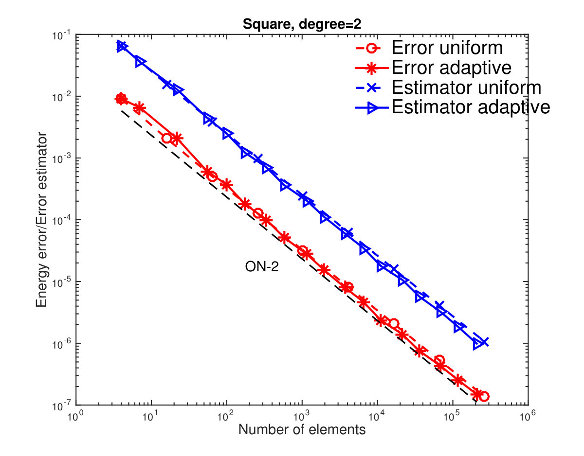 Figure 1
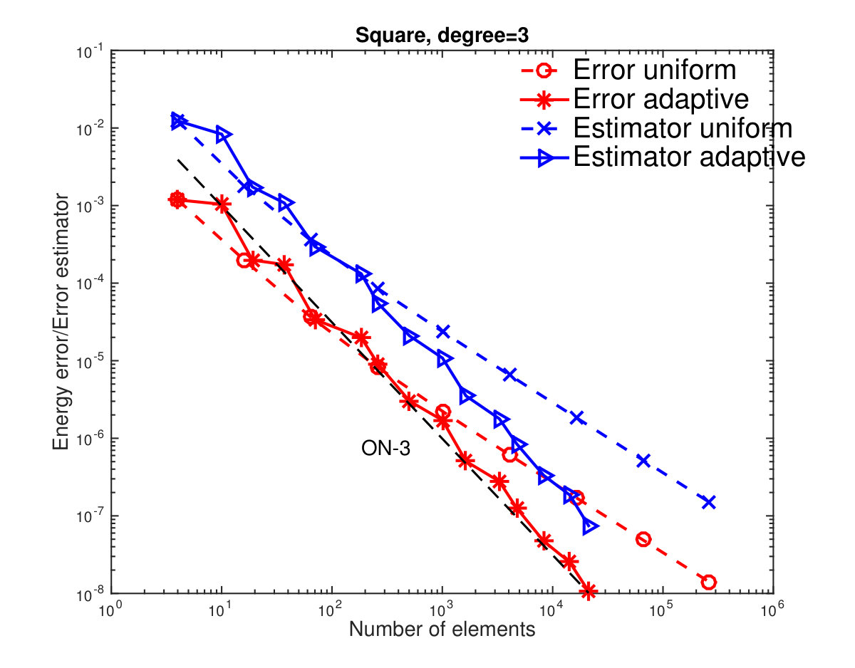 Figure 2
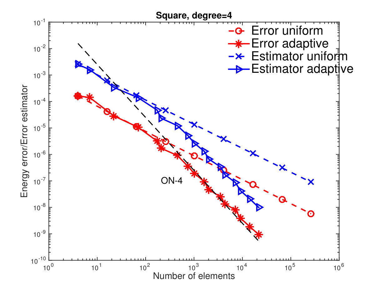 Figure 3
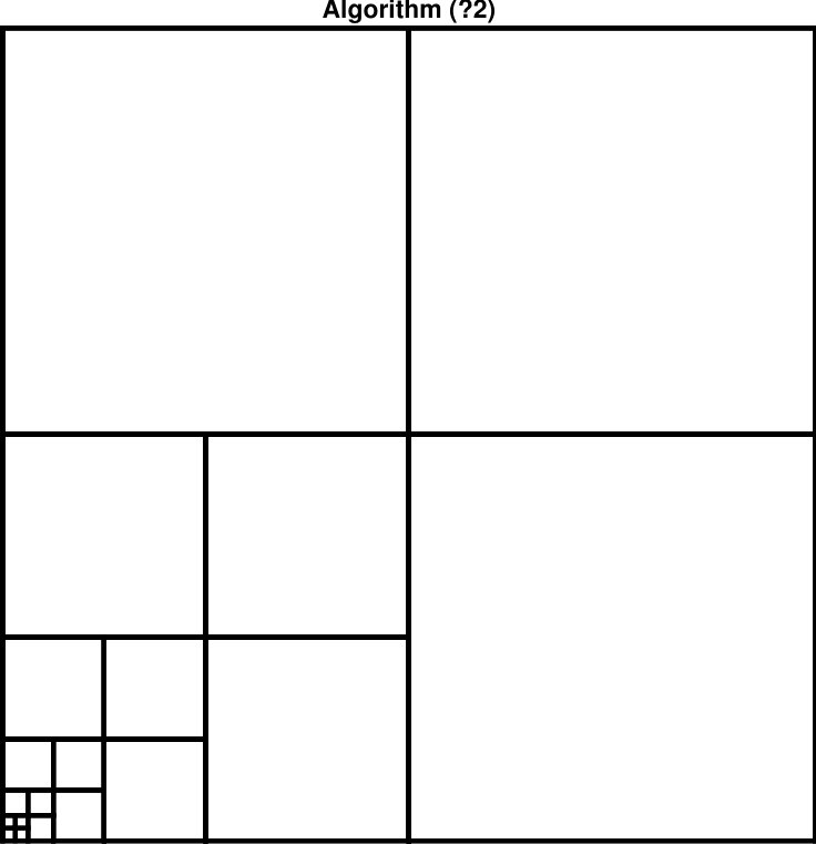 Figure 4
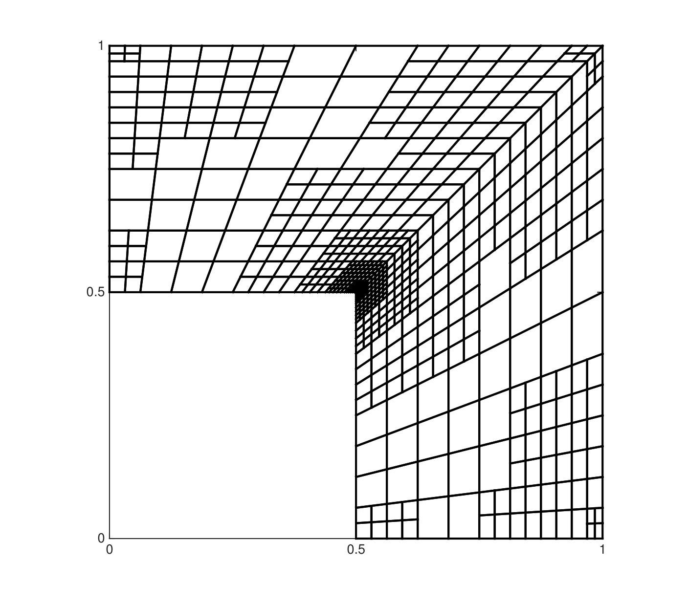 Figure 5
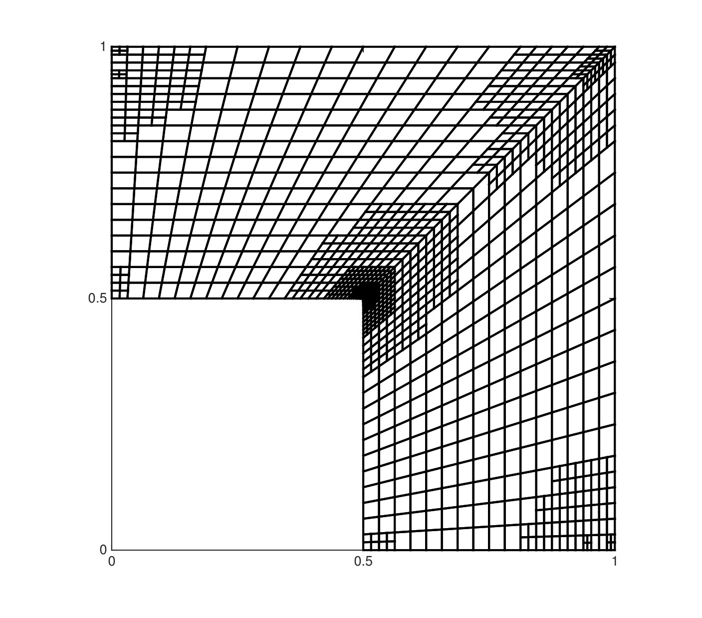 Figure 6
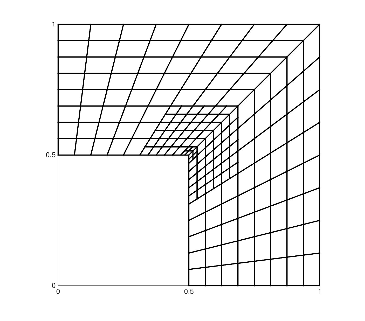 Figure 7
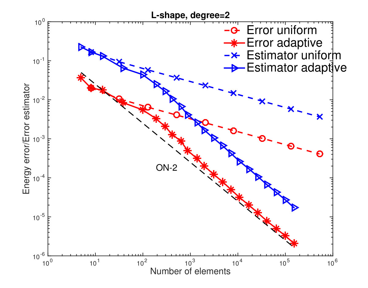 Figure 8
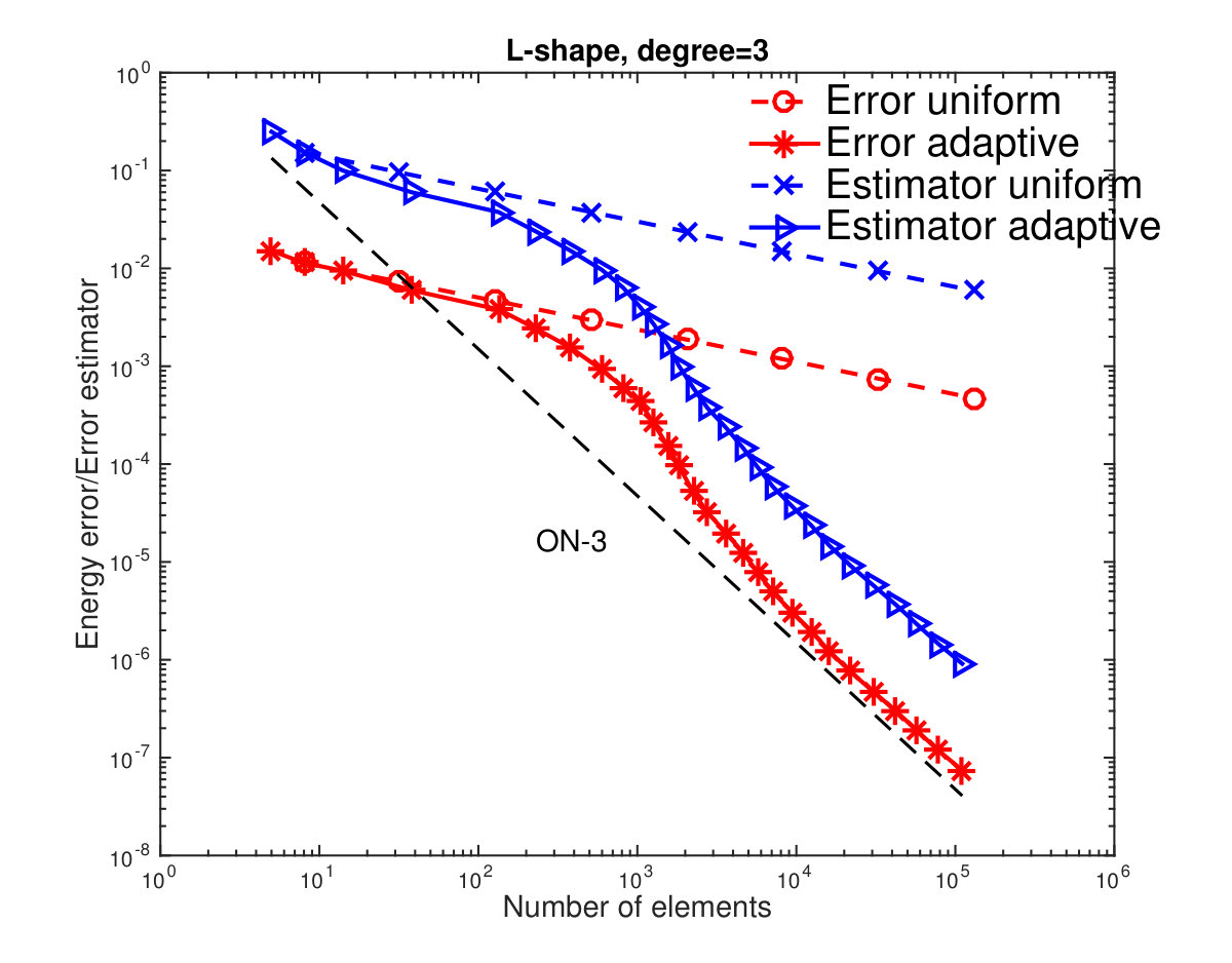 Figure 9
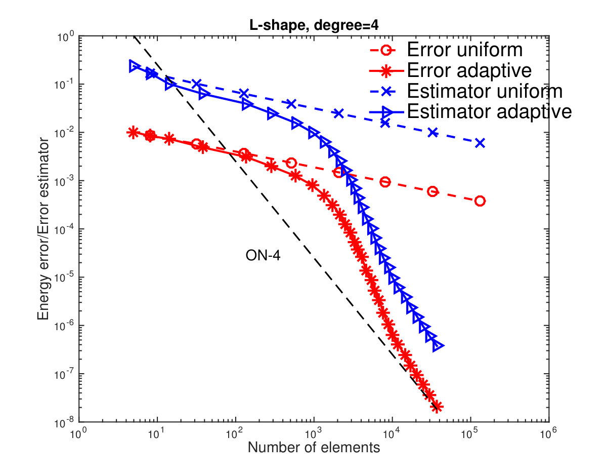 Figure 10
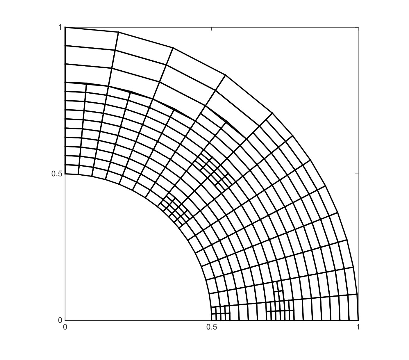 Figure 11
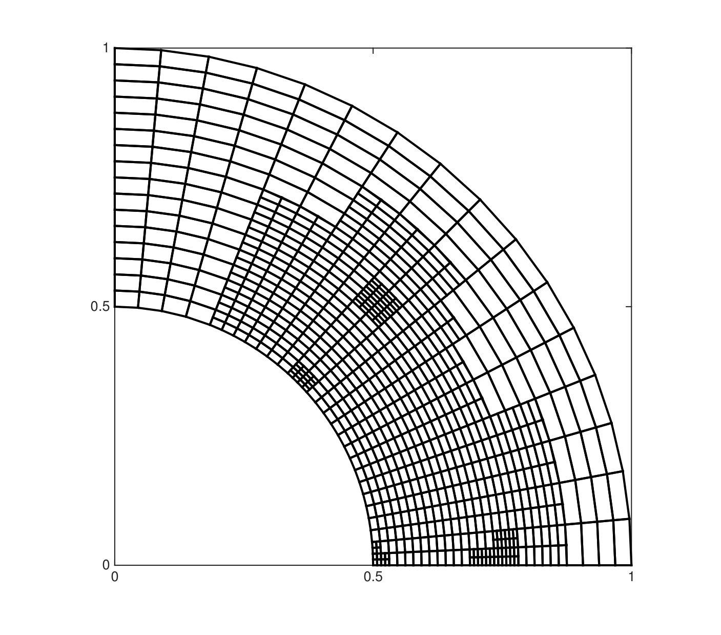 Figure 12
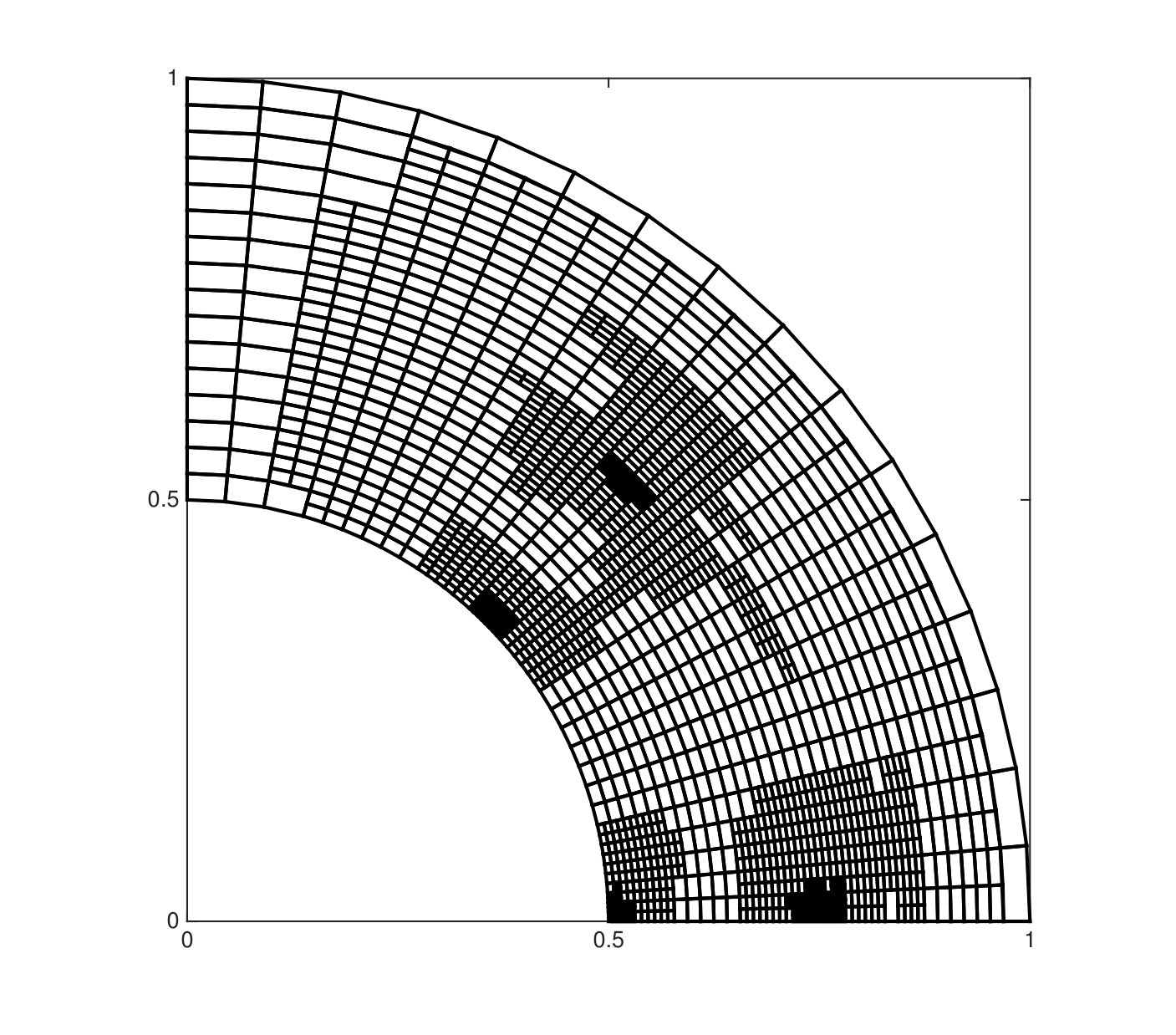 Figure 13
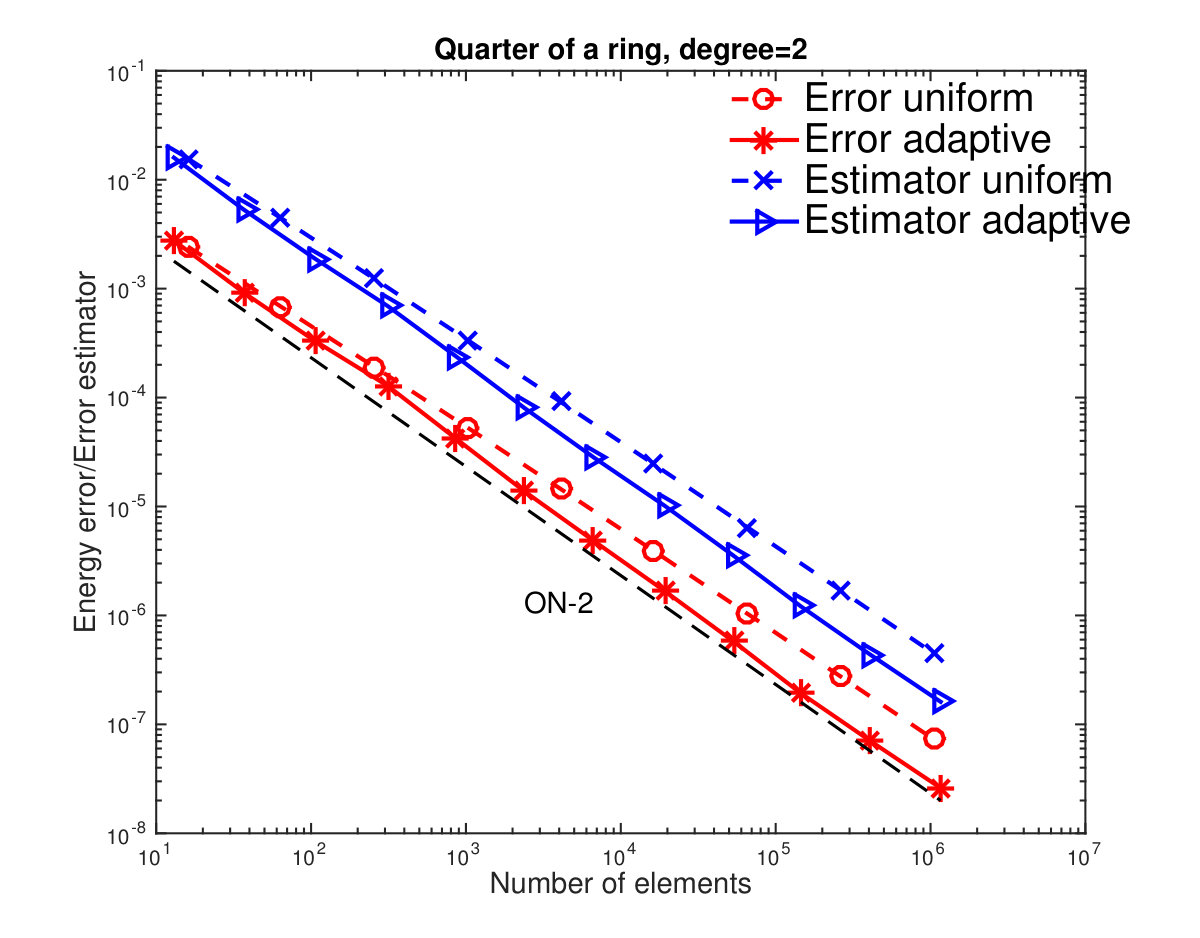 Figure 14
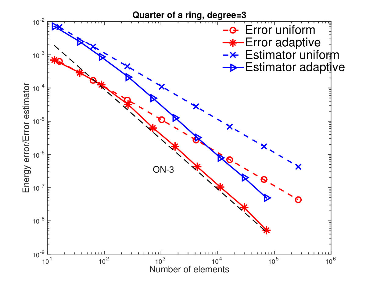 Figure 15
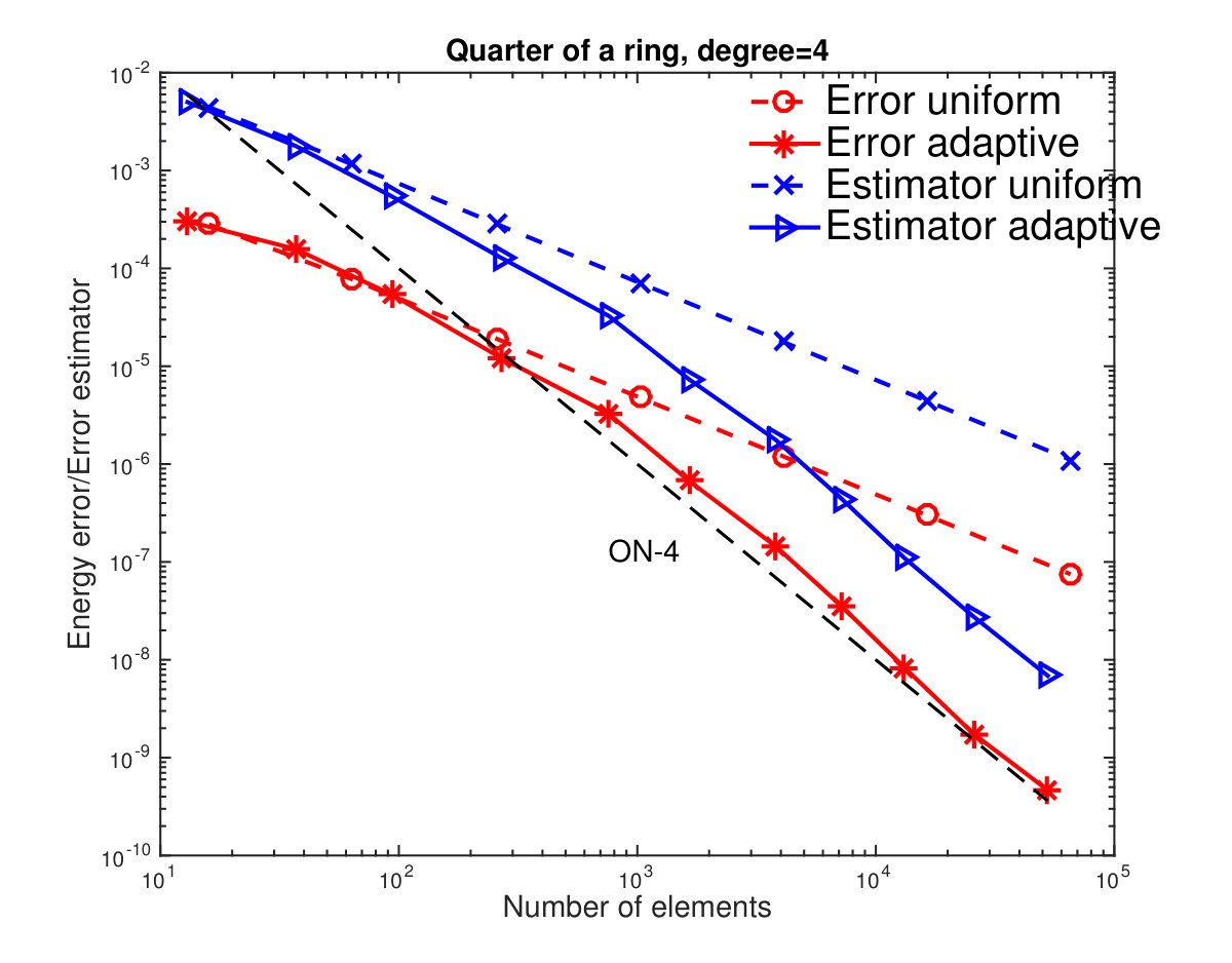 Figure 16
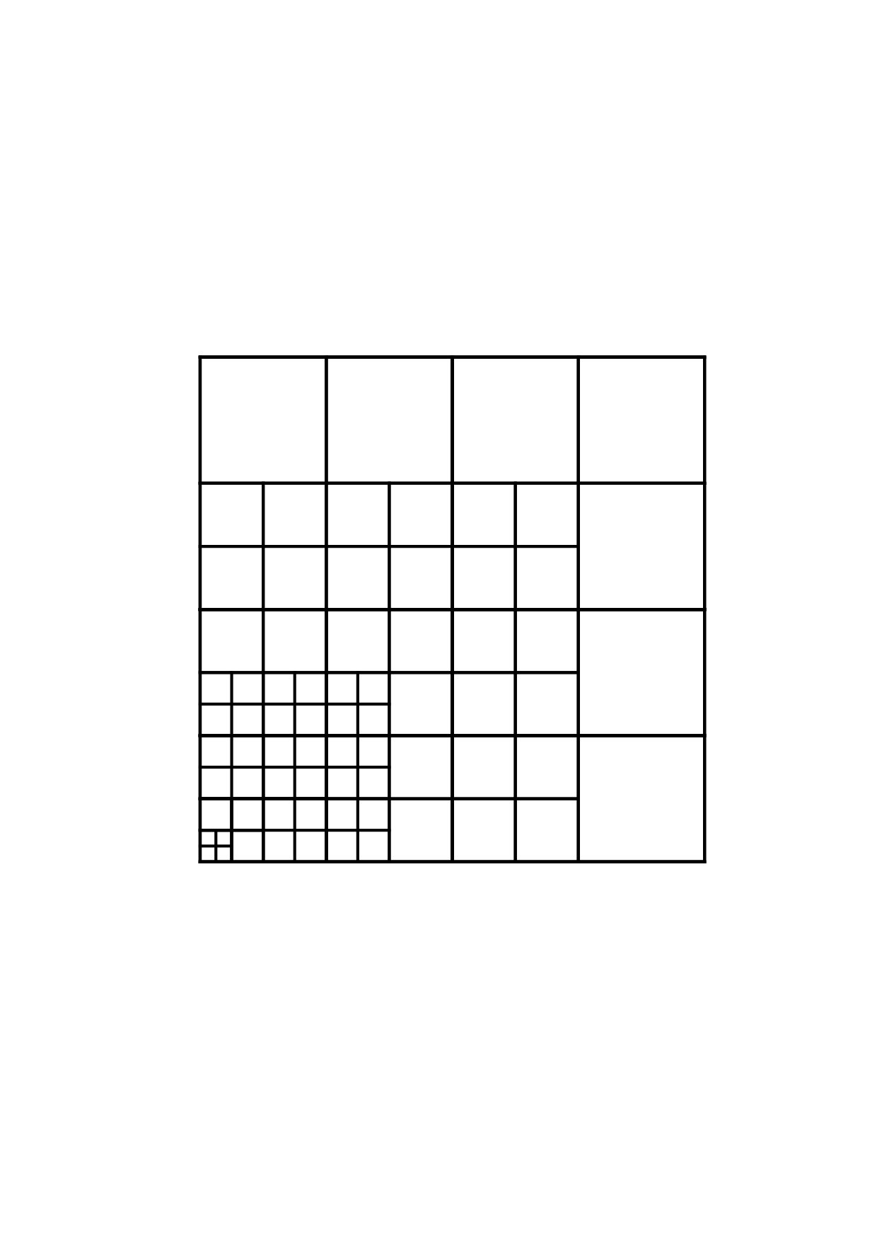 Figure 17
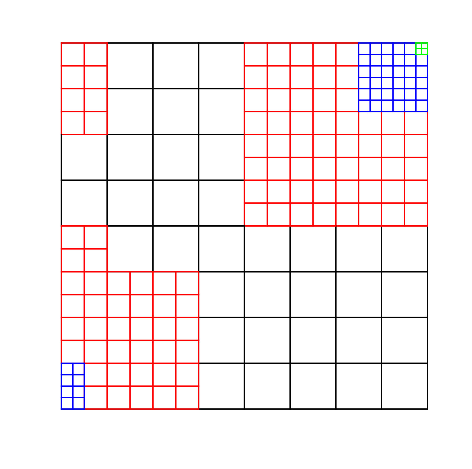 Figure 18
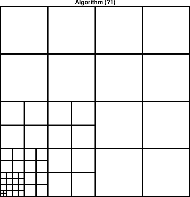 Figure 19
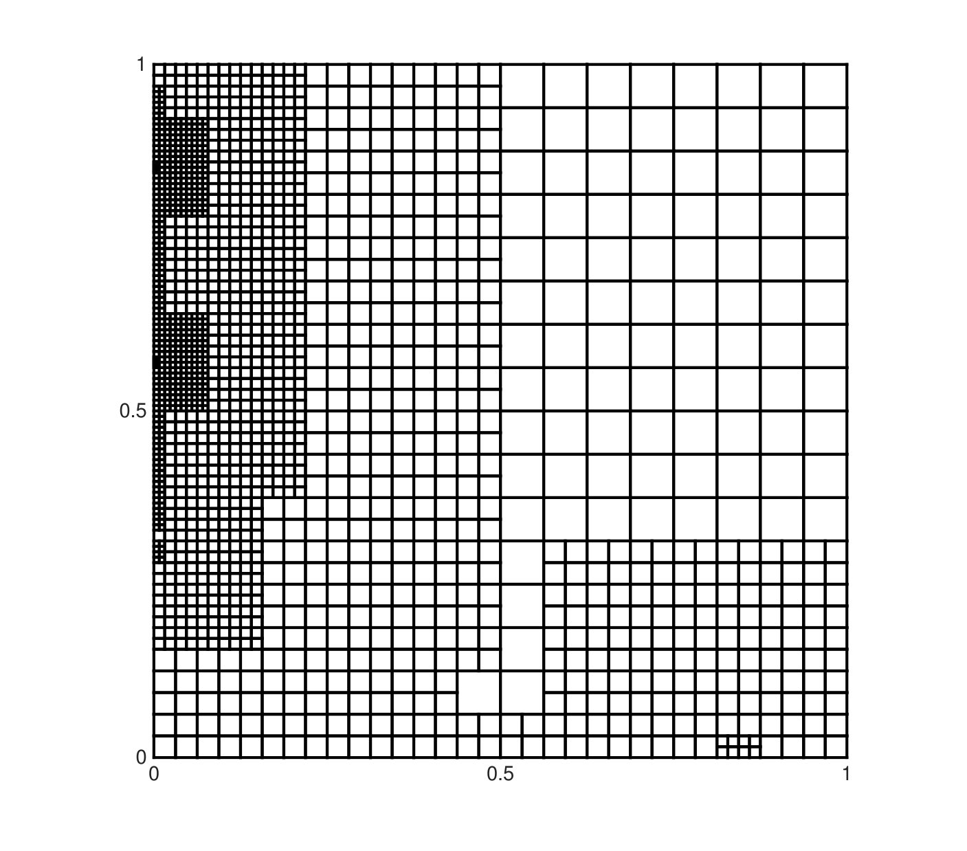 Figure 20
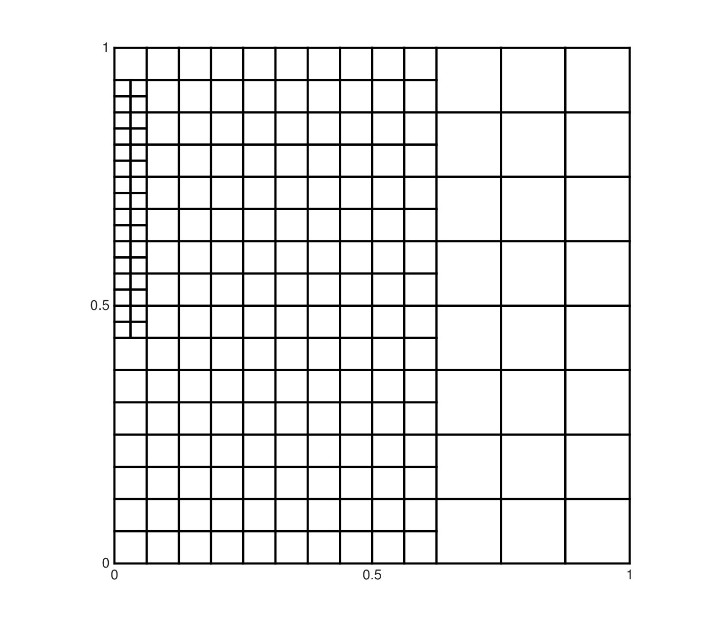 Figure 21
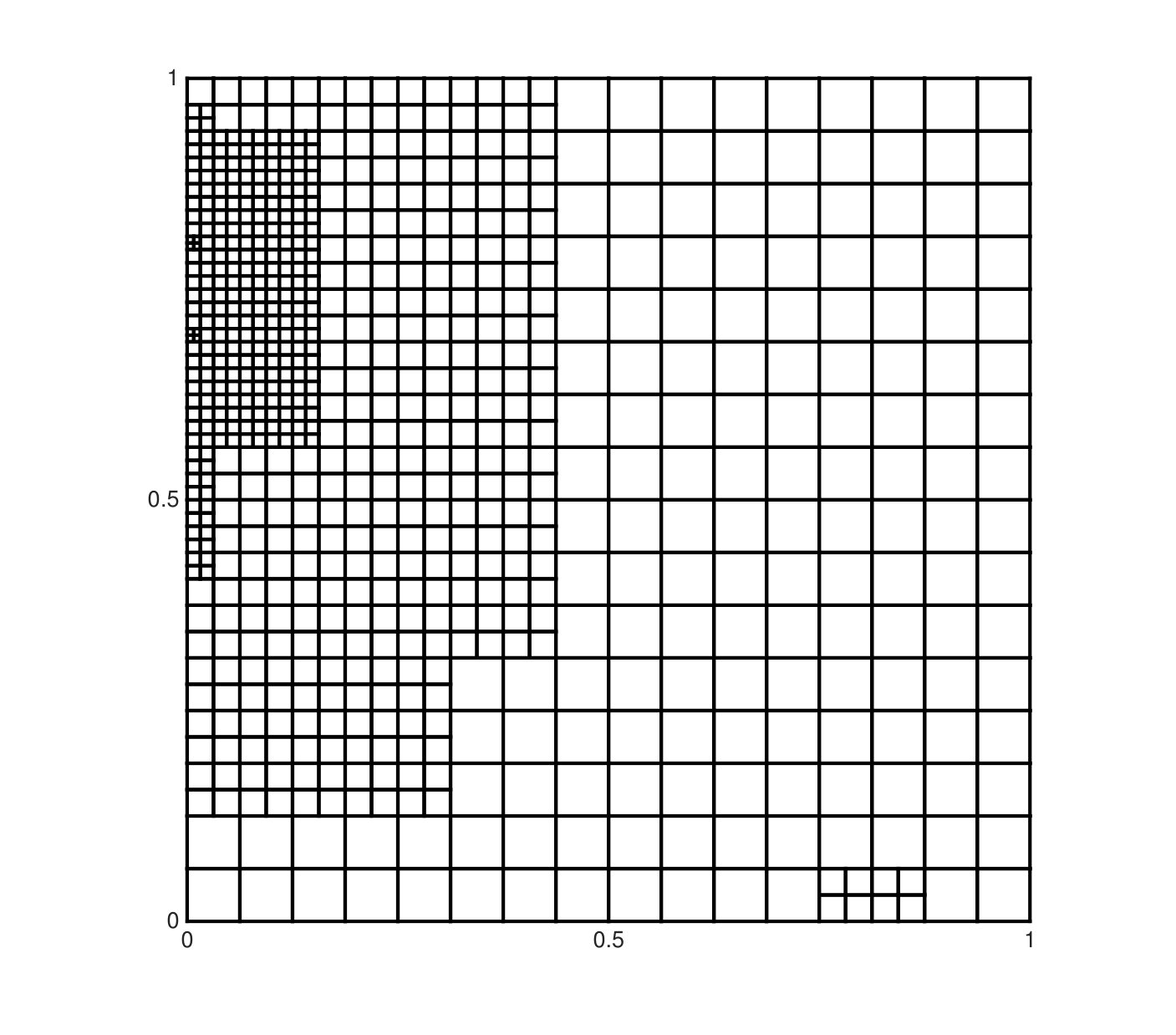 Figure 22