An H^1-conforming Virtual Element Method for Darcy equations and Brinkman equations
Giuseppe Vacca

TL;DR
This paper introduces an H^1-conforming Virtual Element Method for Darcy and Brinkman equations, achieving optimal convergence and stability across different flow regimes with rigorous analysis and numerical validation.
Contribution
It develops a new Virtual Element space with computable projections and divergence-free properties, applicable to both Darcy and Brinkman equations, ensuring stability and optimal convergence.
Findings
Optimal order convergence for Darcy equations
Stable and robust method for Brinkman equations
Numerical tests confirm theoretical error estimates
Abstract
The focus of the present paper is on developing a Virtual Element Method for Darcy and Brinkman equations. In [15] we presented a family of Virtual Elements for Stokes equations and we defined a new Virtual Element space of velocities such that the associated discrete kernel is pointwise divergence-free. We use a slightly different Virtual Element space having two fundamental properties: the L^2-projection onto P_k is exactly computable on the basis of the degrees of freedom, and the associated discrete kernel is still pointwise divergence-free. The resulting numerical scheme for the Darcy equation has optimal order of convergence and H^1 conforming velocity solution. We can apply the same approach to develop a robust virtual element method for the Brinkman equation that is stable for both the Stokes and Darcy limit case. We provide a rigorous error analysis of the method and several…
Click any figure to enlarge with its caption.
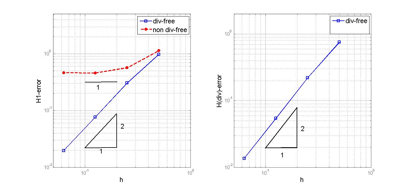 Figure 1
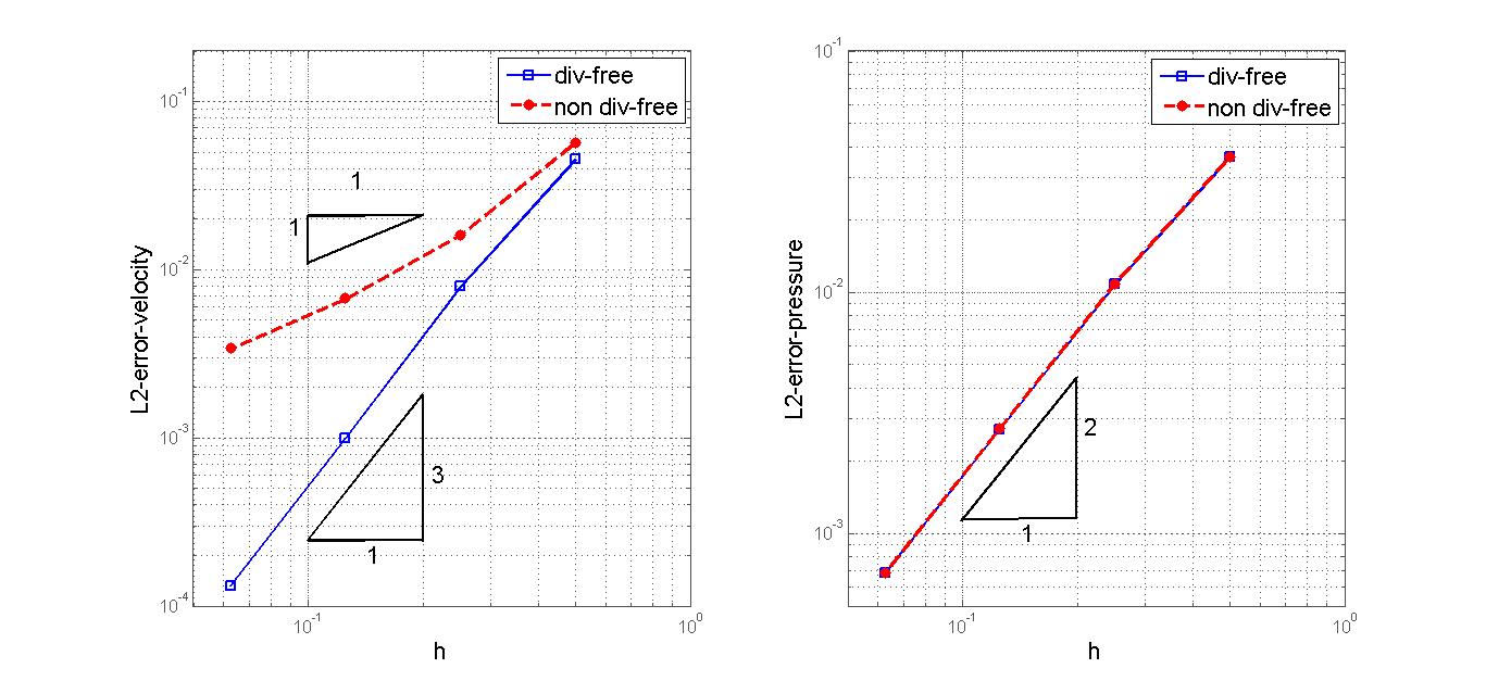 Figure 2
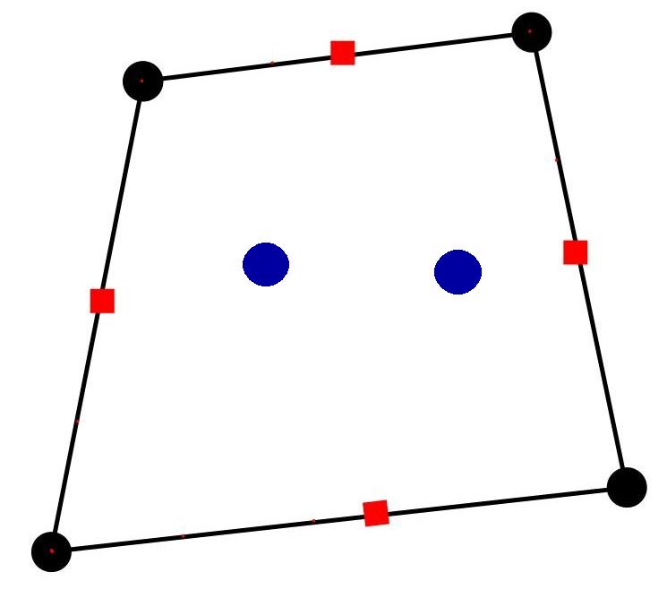 Figure 3
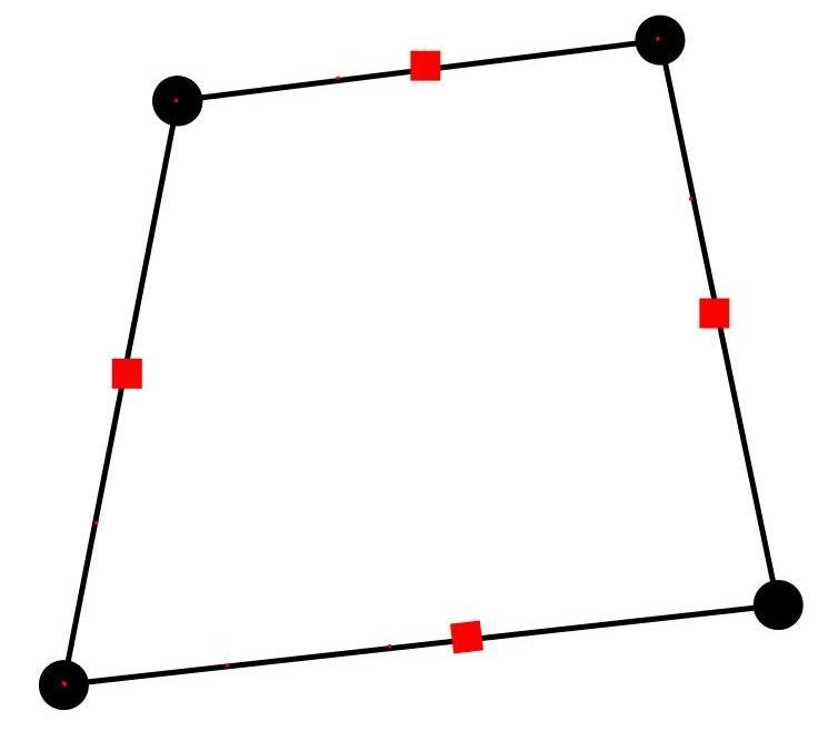 Figure 4
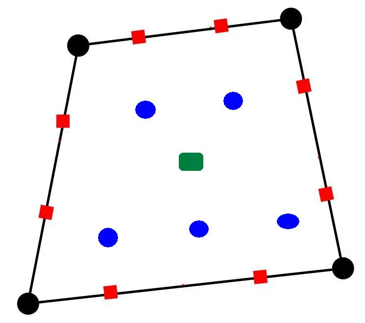 Figure 5
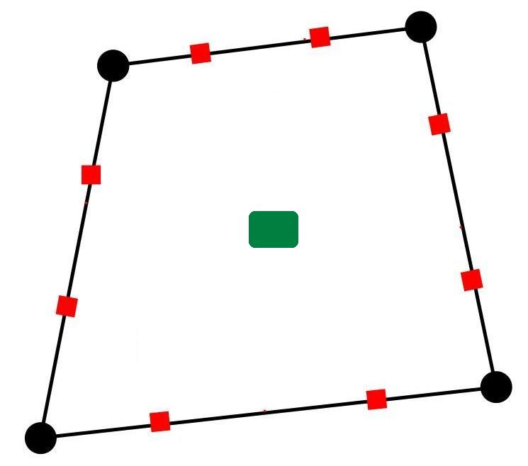 Figure 6
 Figure 7
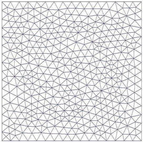 Figure 8
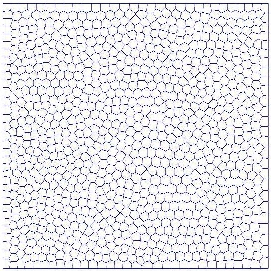 Figure 9
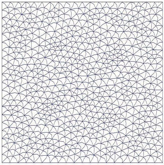 Figure 10
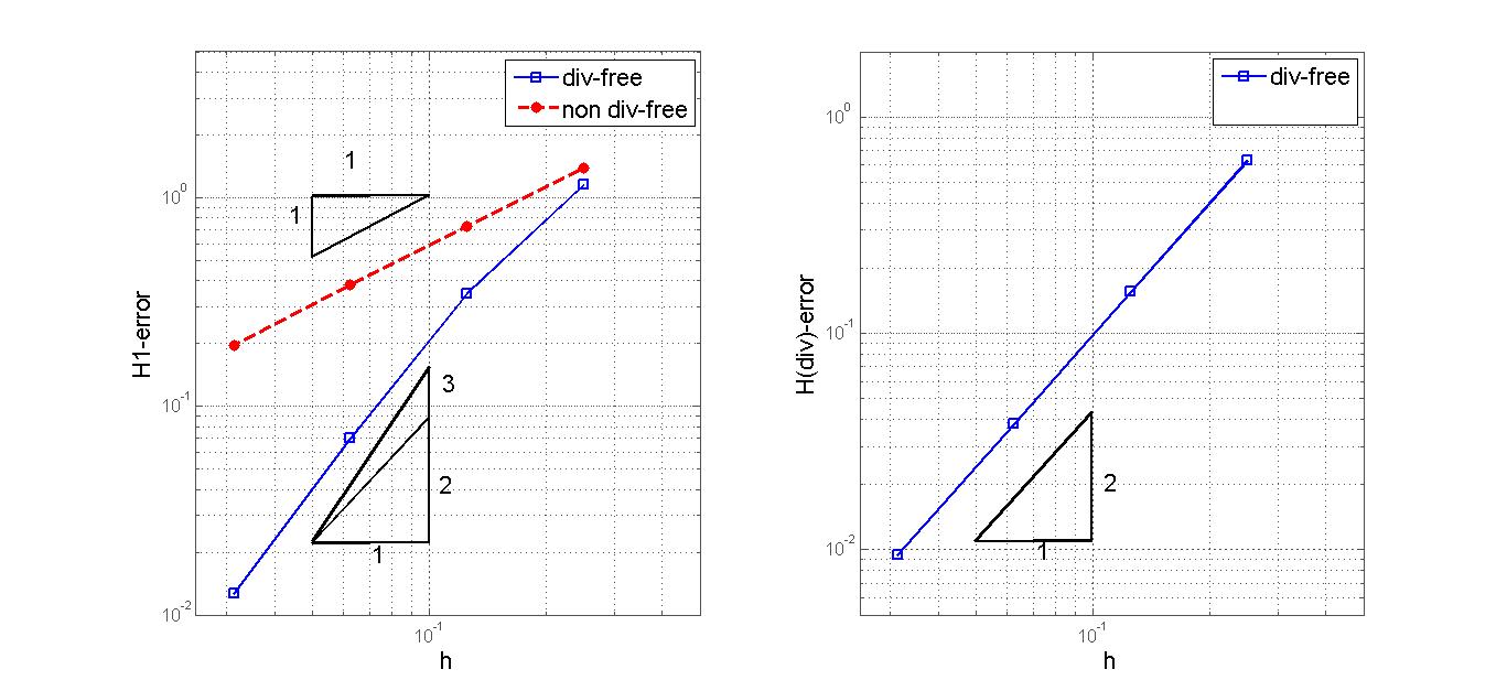 Figure 11
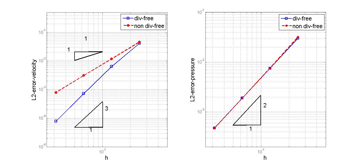 Figure 12
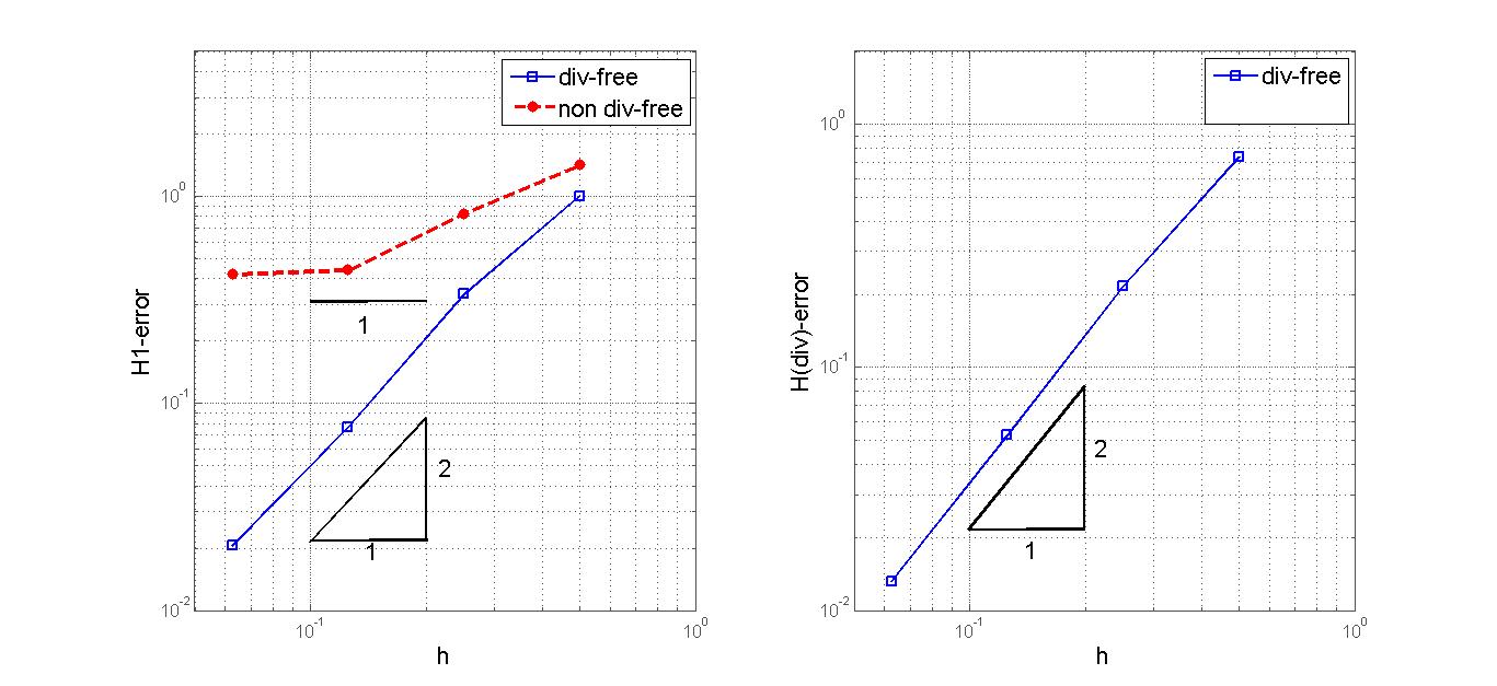 Figure 13
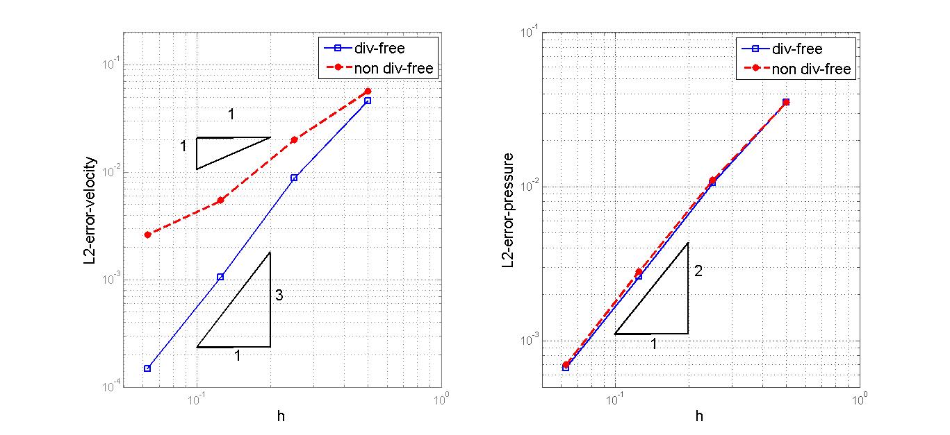 Figure 14
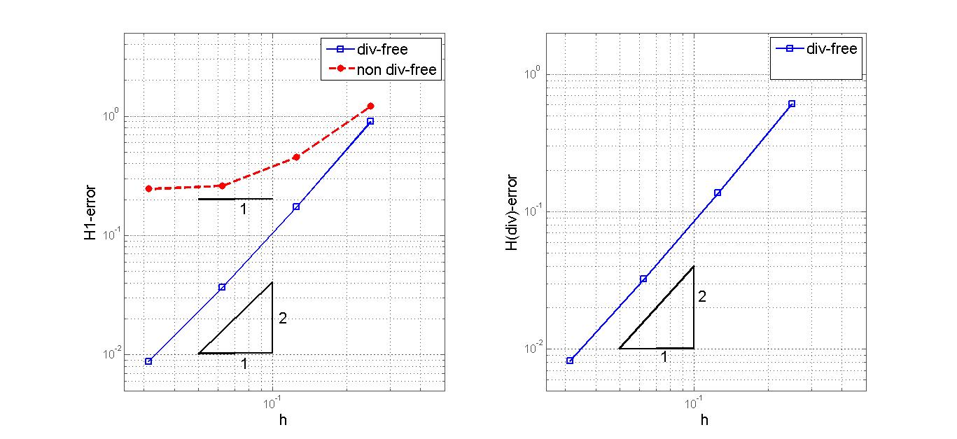 Figure 15
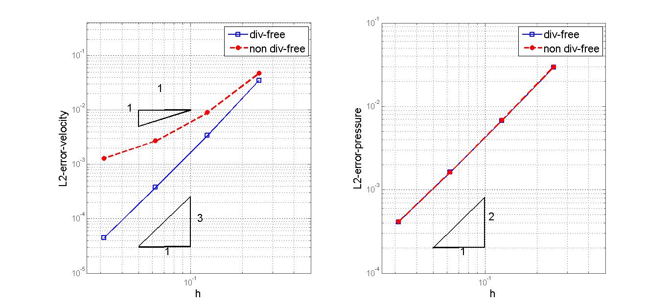 Figure 16
| DoFs | ||||
|---|---|---|---|---|
| DoFs | ||||
|---|---|---|---|---|
Peer Reviews
No public reviews on file for this paper yet. If you reviewed it on a platform where reviews are public (OpenReview, ICLR, NeurIPS, ICML), you can paste yours below so the community can read it here.
Videos
No videos yet. Explain this paper in a talk, walkthrough, or lecture? Add one.
Taxonomy
TopicsNumerical methods in engineering · Advanced Numerical Methods in Computational Mathematics · Model Reduction and Neural Networks
An -conforming Virtual Element Methods for Darcy equations and Brinkman equations
Giuseppe Vacca Dipartimento di Matematica e Applicazioni, Università degli Studi di Milano Bicocca, Via Roberto Cozzi 55 - 20125 Milano, Italy; E-mail: [email protected].
Abstract
The focus of the present paper is on developing a Virtual Element Method for Darcy and Brinkman equations. In [15] we presented a family of Virtual Elements for Stokes equations and we defined a new Virtual Element space of velocities such that the associated discrete kernel is pointwise divergence-free. We use a slightly different Virtual Element space having two fundamental properties: the -projection onto is exactly computable on the basis of the degrees of freedom, and the associated discrete kernel is still pointwise divergence-free. The resulting numerical scheme for the Darcy equation has optimal order of convergence and conforming velocity solution. We can apply the same approach to develop a robust virtual element method for the Brinkman equation that is stable for both the Stokes and Darcy limit case. We provide a rigorous error analysis of the method and several numerical tests.
1 Introduction
The Virtual Element Methods (in short, VEM or VEMs) is a recent technique for solving PDEs. VEMs were recently introduced in [5] as a generalization of the finite element method on polyhedral or polygonal meshes. In the numerical analysis and engineering literature there has been a recent growth of interest in developing numerical methods that can make use of general polygonal and polyhedral meshes, as opposed to more standard triangular/quadrilateral (tetrahedral/hexahedral) grids. Indeed, making use of polygonal meshes brings forth a range of advantages, including for instance automatic hanging node treatment, more efficient approximation of geometric data features, better domain meshing capabilities, more efficient and easier adaptivity, more robustness to mesh deformation, and others. This interest in the literature is also reflected in commercial codes, such as CD-Adapco, that have recently included polytopal meshes.
We refer to the recent papers and monographs [25, 11, 20, 21, 37, 42, 44, 43, 45, 50, 51, 29, 30, 41, 28] as a brief representative sample of the increasing list of technologies that make use of polygonal/polyhedral meshes. We mention here in particular the polygonal finite elements, that generalize finite elements to polygons/polyhedrons by making use of generalized non-polynomial shape functions, and the mimetic discretisation schemes [38, 12], that combine ideas from the finite difference and finite element methods.
The principal idea behind VEM is to use approximated discrete bilinear forms that require only integration of polynomials on the (polytopal) element in order to be computed. The resulting discrete solution is conforming and the accuracy granted by such discrete bilinear forms turns out to be sufficient to achieve the correct order of convergence. Following this approach, VEM is able to make use of very general polygonal/polyhedral meshes without the need to integrate complex non-polynomial functions on the elements and without loss of accuracy. Moreover, VEM is not restricted to low order converge and can be easily applied to three dimensions and use non convex (even non simply connected) elements. The Virtual Element Method has been developed successfully for a large range of problems, see for instance [5, 26, 6, 1, 17, 23, 3, 32, 19, 18, 40, 10, 13, 27, 52, 54, 48, 47, 4, 33, 31]. A helpful paper for the implementation of the method is [7].
The focus of this paper is on developing a new Virtual Element Method for the Darcy equation that is suitable for a robust extension to the (more complex) Brinkman problem. For such a problem, other VEM numerical schemes have been proposed, see for example [23, 8].
In [15] the authors developed a new Virtual Element Method for Stokes problems by exploiting the flexibility of the Virtual Element construction in a new way. In particular, they define a new Virtual Element space of velocities carefully designed to solve the Stokes problem. In connection with a suitable pressure space, the new Virtual Element space leads to an exactly divergence-free discrete velocity, a favorable property when more complex problems, such as the Navier-Stokes problem, are considered. We highlight that this feature is not shared by the method defined in [6] or by most of the standard mixed Finite Element methods, where the divergence-free constraint is imposed only in a weak (relaxed) sense.
In the present contribution we develop the Virtual Element Method for Darcy equations by introducing a slightly different virtual space for the velocities such that the local orthogonal projection onto the space of polynomials of degree less or equal than (where is the polynomial degree of accuracy of the method) can be computed using the local degrees of freedom. The resulting Virtual Elements family inherits the advantages on the scheme proposed in [15], in particular it yields an exactly divergence-free discrete kernel. Thus we obtain a stable Darcy element that is also uniformly stable for the Stokes problem. A sample of uniformly stable methods for Darcy-Stokes model is for instance [39, 53, 36, 49].
The last part of the paper deals with the analysis of a new mixed finite element method for Brinkman equations that stems from the above scheme for the Darcy problem. Mathematically, the Brinkman problem resembles both the Stokes problem for fluid flow and the Darcy problem for flow in porous media (see [35, 2, 34]). Constructing finite element methods to solve the Brinkman equation that are robust for both (Stokes and Darcy) limits is challenging. We will see how the above Virtual Element approach offers a natural and straightforward framework for constructing stable numerical algorithms for the Brinkman equations.
We remark that the proposed scheme belongs to the class of the pressure-robust method, i.e. delivers a velocity error independent of the continuous pressure.
The paper is organized as follows. In Section 2 we introduce the model continuous Darcy problem. In Section 3 we present its VEM discretisation. In Section 4 we detail the theoretical features and the convergence analysis of the problem. In Section 5 we develop a stable numerical methods for Brinkman equations. In Section 6 we show the numerical tests. Finally in the Appendix we present the theoretical analysis of the extension to the Darcy equation of the scheme of [6]. Even though this latter method is not recommended for the Darcy problem, the numerical experiments showed an unexpected optimal convergence rate for the pressure. We theoretically prove this behaviour, developing an inverse inequality for the VEM space, which is interesting on its own.
2 The continuous problem
We consider the classical Darcy equation that describes the flow of a fluid through a porous medium. Let be a bounded polygon then the Darcy equation in mixed form is
[TABLE]
where and are respectively the velocity and the pressure fields, is the source term and is a uniformly symmetric, positive definite tensor that represents the permeability of the medium. From (1), since we have assumed no flux boundary conditions all over , the external force has zero mean value on . We consider the spaces
[TABLE]
equipped with the natural norms
[TABLE]
and the bilinear forms and defined by:
[TABLE]
[TABLE]
Then the variational formulation of Problem (1) is
[TABLE]
where
[TABLE]
Let us introduce the kernel
[TABLE]
then it is straightforward to see that
[TABLE]
It is well known that (see for instance [24]):
- •
and are continuous, i.e.
[TABLE]
[TABLE]
- •
is coercive on the kernel , i.e. there exists a positive constant depending on such that
[TABLE]
- •
satisfies the inf-sup condition, i.e.
[TABLE]
Therefore, Problem (4) has a unique solution such that
[TABLE]
with the constant depending only on and .
3 Virtual formulation for Darcy equations
3.1 Decomposition and the original virtual element spaces
We outline the Virtual Element discretization of Problem (4). Here and in the rest of the paper the symbol will indicate a generic positive constant independent of the mesh size that may change at each occurrence. Moreover, given any subset in and , we will denote by the polynomials of total degree at most defined on , with the extended notation . Let be a sequence of decompositions of into general polygonal elements with
[TABLE]
We suppose that for all , each element in fulfils the following assumptions:
- •
is star-shaped with respect to a ball of radius ,
- •
the distance between any two vertexes of is ,
where and are positive constants. We remark that the hypotheses above, though not too restrictive in many practical cases, can be further relaxed, as noted in [5, 14]. From now on we assume that is piecewise constant with respect to on .
Using standard VEM notation, for , let us define the spaces
- •
the set of polynomials on of degree ,
- •
,
- •
,
- •
with .
In [15] the authors have introduced a new family of Virtual Elements for the Stokes problem on polygonal meshes. In particular, by a proper choice of the Virtual space of velocities, the virtual local spaces are associated to a Stokes-like variational problem on each element. The main ideas of the method are
- •
the Virtual space contains the space of all the polynomials of the prescribed order plus suitable non polynomial functions,
- •
the degrees of freedom are carefully chosen so that the semi-norm projection onto the space of polynomials can be exactly computed,
- •
the choice of the Virtual space of velocities and the associated degrees of freedom guarantee that the final discrete velocity is pointwise divergence-free and more generally the discrete kernel is contained in the continuous one.
In this section we briefly recall from [15] the notations, the main properties of the Virtual spaces and some details of the construction of the semi-norm projection. Let the polynomial degree of accuracy of the method, then we define on each element the finite dimensional local virtual space
[TABLE]
where all the operators and equations above are to be interpreted in the distributional sense. It is easy to check that , and that (see [15] for the proof) the dimension of is
[TABLE]
The corresponding degrees of freedom are chosen prescribing, given a function , the following linear operators , split into four subsets (see Figure 1):
- •
: the values of at the vertices of the polygon ,
- •
: the values of at distinct points of every edge (for example we can take the internal points of the -Gauss-Lobatto quadrature rule in , as suggested in [7]),
- •
: the moments of
[TABLE]
- •
: the moments up to order and greater than zero of in , i.e.
[TABLE]
For all , we introduce the semi-norm projection , defined by
[TABLE]
where is the -projection operator onto the constant functions defined on . It is immediate to check that the energy projection is well defined and it clearly holds for all . Moreover the operator is computable in terms of the degrees of freedom (see equations in [15] and the subsequent discussion).
3.2 The modified virtual space and the projection
Let a positive integer, then for all , the -projection is defined by
[TABLE]
It is possible to check (see Section 3.3 of [15] for the proof) that the degrees of freedom allow us to compute exactly the -projection . On the other hand we can observe that we can not compute exactly from the DoFs the -projection onto the space of polynomials of degree . The goal of the present section is to introduce, taking the inspiration from [1], a new virtual space to be used in place of in such a way that
- •
the DoFs can still be used for ,
- •
,
- •
the projection can be exactly computable by the DoFs .
To construct we proceed as follows: first of all we define an augmented virtual local space by taking
[TABLE]
Now we define the enhanced Virtual Element space as the restriction of given by
[TABLE]
where the symbol denotes the polynomials in that are orthogonal to all polynomials of . We proceed by investigating the dimension and by choosing suitable DoFs of the virtual space . First of all we recall from [9] the following facts
[TABLE]
where is the number of edges of the polygon .
Lemma 3.1**.**
The dimension of is
[TABLE]
Moreover as DoFs for we can take the linear operators and plus the moments
[TABLE]
Proof.
The proof is virtually identical to that given in [15] for and it is based (see for instance [24]) on the fact that given
- •
a polynomial function ,
- •
a polynomial function ,
- •
a polynomial function satisfying the compatibility condition
[TABLE]
there exists a unique pair such that
[TABLE]
Moreover, since from [9], is an isomorphism, we can conclude that the map that associates a given compatible data set to the velocity field that solves (12) is an injective map. Then
[TABLE]
and the thesis follows from (11). ∎
Proposition 3.1**.**
The dimension of is equal to that of that is, as in (8)
[TABLE]
As DoFs in we can take .
Proof.
From (11) it is straightforward to check that
[TABLE]
Hence, neglecting the independence of the additional conditions in (10), it holds that
[TABLE]
We now observe that a function such that is identically zero. Indeed, from (9), it is immediate to check that in this case the would be zero, implying that all its moment are zero, in particular, since , all the moments of are also zero. Now, from Lemma 3.1, we have that is zero. Therefore, from (14), we obtain that the dimension of is actually the same of , and that the DoFs are unisolvent for . ∎
Proposition 3.2**.**
The degrees of freedom allow us to compute exactly the -projection , i.e. the moments
[TABLE]
for all and for all .
Proof.
Let us set
[TABLE]
with , and . Therefore using the Green formula and since , we get
[TABLE]
Now, since is a polynomial of degree less or equal than we can reconstruct its value from and compute exactly the first term. The second term is computable from . The third term is computable from all the using the projection . Finally from and we can reconstruct on the boundary and so compute exactly the boundary term. ∎
For what concerns the pressures we take the standard finite dimensional space
[TABLE]
having dimension
[TABLE]
The corresponding degrees of freedom are chosen defining for each the following linear operators :
- •
: the moments up to order of , i.e.
[TABLE]
Finally we define the global virtual element spaces as
[TABLE]
and
[TABLE]
with the obvious associated sets of global degrees of freedom. A simple computation shows that:
[TABLE]
and
[TABLE]
where is the number of elements, , (resp., , ) is the number of internal edges and vertexes (resp., boundary edges and vertexes) in . As observed in [15], we remark that
[TABLE]
Remark 3.1*.*
By definition (16) it is clear that our discrete velocities field is -conforming, in particular we obtain continuous velocities, whereas the natural discretization is only - conforming. This property, in combination with (18), will make our method suitable for a (robust) extension to the Brinkman problem.
3.3 The discrete bilinear forms
The next step in the construction of our method is to define on the virtual spaces and a discrete version of the bilinear forms and given in (2) and (3). For simplicity we assume that the tensor is piecewise constant with respect to the decomposition , i.e. is constant on each polygon . First of all we decompose into local contributions the bilinear forms and , the norms and by defining
[TABLE]
[TABLE]
and
[TABLE]
We now define discrete versions of the bilinear form (cf. (2)), and of the bilinear form (cf. (3)). For what concerns , we simply set
[TABLE]
i.e. as noticed in [15] we do not introduce any approximation of the bilinear form. We notice that (19) is computable from the degrees of freedom , and , since is polynomial in each element . On the other hand, the bilinear form needs to be dealt with in a more careful way. First of all, by Proposition 3.2, we observe that for all and for all , the quantity
[TABLE]
is exactly computable by the DoFs. However, for an arbitrary pair , the quantity is clearly not computable. In the standard procedure of VEM framework, we define a computable discrete local bilinear form
[TABLE]
approximating the continuous form and satisfying the following properties:
- •
-consistency: for all and
[TABLE]
- •
stability: there exist two positive constants and , independent of and , such that, for all , it holds
[TABLE]
Let be a (symmetric) stabilizing bilinear form, satisfying
[TABLE]
with and positive constants independent of and . Then, we can set
[TABLE]
for all .
It is straightforward to check that Definition (9) and properties (23) imply the consistency and the stability of the bilinear form .
Remark 3.2*.*
In the construction of the stabilizing form with condition (23) we essentially require that the stabilizing term scales as . Following the standard VEM technique (cf. [5, 7] for more details), denoting with , the vectors containing the values of the local degrees of freedom associated to , we set
[TABLE]
where is a suitable positive constant that scales as . For example, in the numerical tests presented in Section 6, we have chosen as the mean value of the eigenvalues of the matrix stemming from the term in (24).
Finally we define the global approximated bilinear form by simply summing the local contributions:
[TABLE]
3.4 The discrete problem
We are now ready to state the proposed discrete problem. Referring to (16), (17), (19), and (25) we consider the virtual element problem:
[TABLE]
We point out that the symmetry of together with (22) easily implies that is (uniformly) continuous with respect to the norm. Moreover, as observed in [15], introducing the discrete kernel:
[TABLE]
it is immediate to check that
[TABLE]
Then the bilinear form is also uniformly coercive on the discrete kernel with respect to the norm. Moreover as a direct consequence of Proposition 4.3 in [15], we have the following stability result.
Proposition 3.3**.**
Given the discrete spaces and defined in (16) and (17), there exists a positive , independent of , such that:
[TABLE]
In particular, the the inf-sup condition of Proposition 3.3, along with property (18), implies that:
[TABLE]
Finally we can state the well-posedness of virtual problem (26).
Theorem 3.1**.**
Problem (26) has a unique solution , verifying the estimate
[TABLE]
4 Theoretical results
We begin by proving an approximation result for the virtual local space . First of all, let us recall a classical result by Brenner-Scott (see [22]).
Lemma 4.1**.**
Let , then for all with , there exists a polynomial function , such that
[TABLE]
We have the following approximation results (for the proof see [16]).
Proposition 4.1**.**
Let with . Under the assumption and on the decomposition , there exists such that
[TABLE]
where is a constant independent of .
For what concerns the pressures, from classic polynomial approximation theory [22], for it holds
[TABLE]
We are ready to state the following convergence theorem.
Theorem 4.1**.**
Let be the solution of problem (4) and be the solution of problem (26). Then it holds
[TABLE]
Proof.
We begin by remarking that as a consequence of the inf-sup condition with classical arguments (see for instance Proposition 2.5 in [24]), there exists such that
[TABLE]
Let us set . From (30) and (26), we have that and thus . Now, using (5), (22), (26) and introducing the piecewise polynomial approximation (28) together with (21), we have
[TABLE]
then
[TABLE]
The -estimate follows easily by the triangle inequality. It is also straightforward to see from (4) and (26) that
[TABLE]
than we get for all and therefore
[TABLE]
from which the estimate in the norm. We proceed by analysing the error on the pressure field. Let , then from the discrete inf-sup condition (27), we infer:
[TABLE]
Since and are respectively the solution of (4) and (26), it follows that
[TABLE]
Therefore, we get
[TABLE]
Using (21), the continuity of and the triangle inequality, we get:
[TABLE]
where is the piecewise polynomial of degree defined in Lemma 4.1. Then, from estimate (28) and the previous estimate on the velocity error, we obtain
[TABLE]
Moreover, we have
[TABLE]
Then, using (33) and (34) in (32), we infer
[TABLE]
Finally, using (35) and the triangular inequality, we get
[TABLE]
Passing to the infimum with respect to , and using estimate (29), we get the thesis. ∎
Remark 4.1*.*
We observe that the estimates on the velocity errors in Theorem 4.1 do not depend on the continuous pressure, whereas the velocity errors of the classical methods have a pressure contribution. Therefore the proposed scheme belongs to the class of the pressure-robust methods.
5 A Stable VEM for Brinkman Equations
5.1 The continuous problem
The Brinkman equation describes fluid flow in complex porous media with a viscosity coefficient highly varying so that the flow is dominated by the Darcy equations in some regions of the domain and by the Stokes equation in others. We consider the Brinkman equation on a polygon with homogeneous Dirichlet boundary conditions:
[TABLE]
where and are the unknown velocity and pressure fields, is the fluid viscosity, denotes the permeability tensor of the porous media and is the external source term. We assume that is a symmetric positive definite tensor and that there exist two positive (uniform) constants , such that
[TABLE]
For what concerns the fluid viscosity we consider , this include the case where approaches zero and equation (36) becomes a singular perturbation of the classic Darcy equations. Let us consider the spaces
[TABLE]
with the usual norms, and let be the bilinear form defined by:
[TABLE]
where
[TABLE]
and is the bilinear form defined in (2). Then the variational formulation of Problem (36) is:
[TABLE]
where and is the bilinear form in (3) and using standard notation
[TABLE]
The natural energy norm for the velocities is induced by the symmetric an positive bilinear form and is defined by (e.g. [35])
[TABLE]
We can observe that the equivalence with the norm is not uniform, i.e.
[TABLE]
where , here and in the follows denote two positive constant independent of and . For what concerns the pressures, we consider the norm (see for instance [35])
[TABLE]
Using the inf-sup condition in the usual norm it is possible to check the equivalence between the norms for the pressure but again the equivalence is not uniform, i.e.
[TABLE]
Since, considering the modified norm, the bilinear form is uniformly continuous and coercive, and inf-sup condition is clearly fulfilled, Problem (37) has a unique solution such that
[TABLE]
where the constant depends only on .
5.2 Virtual formulation for Brinkman equations
Mathematically, Brinkman equations can be viewed as a combination of the Stokes and the Darcy equation, that can change from place to place in the computational domain. Therefore, numerical schemes for Brinkman equations have to be carefully designed to accommodate both Stokes and Darcy simultaneously. In this section we propose a Virtual Element scheme that is accurate for both Darcy and Stokes flows. For this goal we combine the ideas developed in the previous sections with the argument in [15].
Let us consider the virtual spaces and (cfr. (16) and (17)). As usual in the VEM framework we need to define a computable approximation of the continuous bilinear forms. Using obvious notations we split the bilinear form as
[TABLE]
We begin by observing that, from [15] (in particular c.f. ) and from Section 3.2, is computable on the basis of the DoFs for all and for all . Starting from this observation we can approximate the continuous form with the bilinear form , given by
[TABLE]
where is the bilinear form defined in equation in [15] and is defined in (20). It is clear that the bilinear form satisfies the -consistency and the stability properties. As usual we build the global approximated bilinear form by simply summing the local contributions. For what concerns the bilinear form , as observed in Section 3.3, it can be computed exactly. The last step consists in constructing a computable approximation of the right-hand side in (37). We define the approximated load term as
[TABLE]
and consider:
[TABLE]
We observe that (40) can be exactly computed from for all (see Proposition 3.2). Furthermore, the following result concerning a and -type norm, can be proved using standard arguments [5].
Lemma 5.1**.**
Let be defined as in (39), and let us assume . Then, for all , it holds
[TABLE]
In the light of the previous definitions, we consider the virtual element approximation of the Brinkman problem:
[TABLE]
Equation (41) is well posed since the discrete bilinear form is (uniformly) stable with respect to the norm by construction and the inf-sup condition is fulfilled (the proof follows the guidelines of Proposition 4.2 in [15] and the linearity of the Fortin operator). Then we have the following result.
Theorem 5.1**.**
Problem (41) has a unique solution , verifying the estimate
[TABLE]
We now notice that, if is the velocity solution to Problem (37), then it is the solution to Problem:
[TABLE]
Analogously, if is the velocity solution to Problem (41), then it is the solution to Problem:
[TABLE]
For what concerns the convergence results we state the following theorem. The proof can be derived by extending the techniques of the previous section and is therefore omitted.
Theorem 5.2**.**
Let be the solution of problem (42) and be the solution of problem (43). Then
[TABLE]
Let be the solution of Problem (37) and be the solution of Problem (41). Then it holds:
[TABLE]
The constants above are independent of and .
In the last part of this section we present a brief discussion about the construction of a reduced virtual element method for Brinkman equations equivalent to Problem (41) but involving significantly fewer degrees of freedom, especially for large . This construction essentially follows the guidelines of Section 5 in [15] (where we refer the reader for a deeper presentation). Let us define the original reduced local virtual spaces, for :
[TABLE]
As before we enlarge the virtual space and we consider
[TABLE]
Finally we define the enhanced Virtual Element space, the restriction of given by
[TABLE]
where as before the symbol denotes the polynomials i that are orthogonal to all polynomials of . For the pressures we consider the reduced space
[TABLE]
As sets of degrees of freedom for the reduced spaces, combining the argument in Section 3 and [15] we may consider the following. For every function we take the following linear operators , split into three subsets (see Figure 2):
- •
: the values of at each vertex of the polygon ,
- •
: the values of at distinct points of every edge ,
- •
: the moments of
[TABLE]
For every we consider
- •
: the moment
[TABLE]
Therefore we have that:
[TABLE]
and
[TABLE]
where is the number of vertexes in .
We define the global reduced virtual element spaces in the standard fashion. The reduced virtual element discretization of the Brinkman problem (37) is then:
[TABLE]
Above, the bilinear forms and , and the loading term are the same as before. The following proposition states the relation between Problem (41) and the reduced Problem (44) (the proof is equivalent to that of Proposition 5.1 in [15]).
Proposition 5.1**.**
Let be the solution of problem (41) and be the solution of problem (44). Then
[TABLE]
6 Numerical tests
In this section we present two numerical experiments to test the practical performance of the method. The first experiment is focused on the method introduced in Section 3 for the Darcy Problem, whereas in the second experiment we test the method in Section 5 for the Brinkman equations.
Since the VEM velocity solution is not explicitly known point-wise inside the elements, we compute the method error comparing with a suitable polynomial projection of the approximated . In particular we consider the computable error quantities:
[TABLE]
Regarding the computational domain, in our tests we always take the square domain , which is partitioned using the following sequences of polygonal meshes:
- •
: sequence of Voronoi meshes with ,
- •
: sequence of triangular meshes with ,
- •
: sequence of square meshes with .
- •
: sequence of WEB-like meshes with .
An example of the adopted meshes is shown in Figure 3.
For the generation of the Voronoi meshes we use the code Polymesher [46]. The non convex WEB-like meshes are composed by hexagons, generated starting from the triangular meshes and randomly displacing the midpoint of each (non boundary) edge.
Test 6.1*.*
In this example we consider the Darcy problem (4) where we set , and we choose the load term in such a way that the analytical solution is
[TABLE]
We analyse the practical performance of the virtual method by studying the errors versus the diameter of the meshes. In addition we compare the results obtained with the scheme of Section 3, labeled as “div-free”, with those obtained with the method in the Appendix, labeled as “non div-free” (in both cases we consider polynomial degrees ).
Remark 6.1*.*
We notice that the "non div-free" method is a naive extension to the Darcy equation of the inf-sup stable scheme proposed in [6]. Since the scheme lacks a uniform ellipticity-on-the-kernel condition, it is not recommended for the problem under consideration. The purpose of the comparison is thus to underline the importance of the property (cf. Section 3.4) in the present context.
In Figure 4 and 5, we display the results for the sequence of Voronoi meshes . In Figure 6 and 7, we show the results for the sequence of meshes , while in Figure 8 and 9 we plot the results for the sequence of meshes , finally in 10 and 11 we exhibit the results for the sequence of meshes .
We notice that the theoretical predictions of Section 4 and the Appendix are confirmed for both the norm and the norm. Note that for the norm we plot only the error for the “div-free” method since such scheme guarantees by construction, a better approximation of the divergence. Indeed let (resp. ) be the solution obtained with the “div-free” method (“non div-free” method) then satisfies
[TABLE]
whereas satisfies the same equation only in a projected sense, i.e.
[TABLE]
We can observe that the convergence rate of the norm for the pressure is optimal also for the “non div-free” method as proved in the Appendix. Finally, we can observe that using a square mesh decomposition holds a convergence rate that is slightly better than what predicted by the theory.
Test 6.2*.*
In this example we test the Brinkman equation (37) with different values of the fluid viscosity and fixed permeability tensor . We choose the load term and the Dirichlet boundary conditions in such a way that the analytical solution is
[TABLE]
The aim of this test is to check the practical performance of the method introduced in Section 5 in the reduced formulation (c.f. (44). In Table 1 and Table 2 we display the total amount of DoFs and the errors for the family of meshes choosing respectively for the “div-free” method (cf. Section 5) and the “non div-free” method (cf. Reamrk 6.1 and the Appendix). We observe that also in the limit case, when the equation becomes a singular perturbation of the classic Darcy equations (e.g. for “small” ), the proposed “div-free” method preserves the optimal order of accuracy.
7 Acknowledgements
The author wishes to thank L. Beirão da Veiga and C. Lovadina for several interesting discussions and suggestions on the paper. The author was partially supported by the European Research Council through the H2020 Consolidator Grant (grant no. 681162) CAVE, Challenges and Advancements in Virtual Elements. This support is gratefully acknowledged.
Appendix: Non divergence-free virtual space
We have built a new -conforming (vector valued) virtual space for the velocity vector field different from the more standard one presented in [6] for the elasticity problem. The topic of the present section is to analyse the extension to the Darcy equation of the scheme of [6]. Even though the method should not be used for the Darcy problem (cf. Remark 6.1), the numerical experiments have shown an optimal error convergence rate for the pressure variable. In this Section, we theoretically explain such a behaviour, under a convexity assumption on (essentially, a regularity assumption on the problem). To this end, we develop an inverse estimate for the VEM spaces which is interesting on its own, and can be used in other contexts. We briefly describe the method by making use of various tools from the Virtual Element technology, and we refer the interested reader to the papers [5, 1, 7, 6]) for a deeper presentation. We consider the local virtual space
[TABLE]
with local degrees of freedom :
- •
: the values of at each vertex of the polygon ,
- •
: the values of at distinct points of every edge ,
- •
: the moments of up to order , i.e.
[TABLE]
As observed in [1], the DoFs allow us to compute the operator defined as the analogous of the semi-norm projection (c.f. (9)). For all , the augmented virtual local space is defined by
[TABLE]
Now we define the enhanced Virtual Element space, the restriction of given by
[TABLE]
where the symbol denotes the polynomials of degree living on that are orthogonal to all polynomials of degree on . The enhanced space has three fundamental properties (see [1] for a proof):
- •
,
- •
the set of linear operators constitutes a set of DoFs for the space ,
- •
the -projection operator is exactly computable by the DoFs.
Recalling (13) and from [6] it holds that . For the pressures we use the space of the piecewise polynomials (c.f. (17)). For what concerns the construction of the approximated bilinear forms, it is straightforward to see that
[TABLE]
is computable from the DoFs for all , . Moreover using standard arguments [1, 48] we can define a computable bilinear form
[TABLE]
approximating the continuous form , and satisfying the -consistency (c.f. (21)) and the stability properties (c.f. (22)). Finally we define the global approximated bilinear form by simply summing the local contributions. By construction (see for instance [1]) the discrete bilinear form is (uniformly) stable with respect to the norm. We are now ready to state the proposed discrete virtual element problem:
[TABLE]
We shall first prove an inverse inequality for the virtual element functions in .
Lemma 7.1**.**
Under the assumption , , let and let . Then the following inverse estimate holds
[TABLE]
where the constant is independent of , and .
Proof.
We only sketch the proof, since we follow the guidelines of Lemma 3.1 and 3.3 in [14]. Let , then
[TABLE]
Under the assumption , and by Lemma 3.3 in [14] we get
[TABLE]
where the constant is independent of , and . For what concerns the second addend in the right side of (47), under the assumptions , , and using Lemma 3.1 in [14], for all the following holds: there exists an extension of such that
[TABLE]
where we consider the scaled norm
[TABLE]
By definition it holds
[TABLE]
Now, using the definition (50), an inverse estimate ( is polynomial on ) and the trace theorem [22], it holds that
[TABLE]
for any real . For the last term, using (50), (49) and (48) we get
[TABLE]
From (51) and (52) we can conclude that
[TABLE]
Finally, choosing and collecting (48) and (53) in (47) we have
[TABLE]
from which follows the thesis. ∎
Let us analyse the theoretical properties of the method. We consider the discrete kernel:
[TABLE]
therefore the divergence-free property is satisfied only in a relaxed (projected) sense. As a consequence the bilinear form is not uniformly coercive on the discrete kernel ; nevertheless it holds the following -dependent coercivity property
[TABLE]
that can be derived by using inverse estimate (46). Recalling that is continuous with respect the norm and that the discrete inf-sup condition is fulfilled [6]
[TABLE]
problem (45) has a unique solution but we expect a worse order of accuracy since the bilinear form is not uniformly stable. In fact we have the following convergence results that are, perhaps surprisingly, still optimal in the pressure variable.
Theorem 7.1**.**
Let be the solution of problem (4) and be the solution of problem (45). Then
[TABLE]
Assuming further that is convex, the following estimate holds:
[TABLE]
Proof.
As observed in the proof of Theorem 4.1 the inf-sup condition (55) implies the existence of a function such that
[TABLE]
Now let us set . For what concerns the norm, using the stability of the bilinear form and (45) together with (4)
[TABLE]
By (45) and property (56), it is straightforward to see that
[TABLE]
so that . Therefore
[TABLE]
for all . Using the inverse estimate (46) and standard approximation theory we get
[TABLE]
By standard technique in VEM convergence theory, it holds that
[TABLE]
Collecting (59) and (60) in (58) we get the estimate. Whereas the norm estimate follows from an inverse estimate (46).
For what concerns the estimate on the pressure, let the piecewise polynomial with respect to defined by for all . Let us set
[TABLE]
From (4) and (45), it is straightforward to see that the couple solves the Darcy problem
[TABLE]
To prove the estimate for the pressure we employ the usual duality argument. Let therefore be the solution of the auxiliary problem
[TABLE]
that, due to the convexity assumption, satisfies
[TABLE]
where the constant depends only on . For all let us denote with its interpolant defined in (56) and (57). Therefore Green formula together with (61) yields
[TABLE]
We analyse separately the three terms. For the first one, using the consistency property of , the polynomial approximation of and , the estimate on the velocity error and (62) we get
[TABLE]
For what concerns the second term we have
[TABLE]
Finally, for the third term we begin by observing that from (61)
[TABLE]
for all , and by the Green formula
[TABLE]
Therefore, by collecting (66), (67), and using the previous error estimate, it holds that
[TABLE]
Finally by collecting (64), (65) and (68) in (63) we get the thesis. ∎
The reference list from the paper itself. Each links out to its DOI / PubMed record.
- 1[1] B. Ahmad, A. Alsaedi, F. Brezzi, L. D. Marini, and A. Russo. Equivalent projectors for virtual element methods. Comput. Math. Appl. , 66(3):376–391, 2013.
- 2[2] V. Anaya, D. Mora, R. Oyarzúa, and R. Ruiz-Baier. A priori and a posteriori error analysis of a mixed scheme for the Brinkman problem. Numer. Math. , pages 1–37, 2015.
- 3[3] P. F. Antonietti, L. Beirão da Veiga, D. Mora, and M. Verani. A stream virtual element formulation of the Stokes problem on polygonal meshes. SIAM J. Numer. Anal. , 52(1):386–404, 2014.
- 4[4] P. F. Antonietti, S. Giani, and P. Houston. h p ℎ 𝑝 hp -version composite discontinuous Galerkin methods for elliptic problems on complicated domains. SIAM J. Sci. Comput. , 35(3):A 1417–A 1439, 2013.
- 5[5] L. Beirão da Veiga, F. Brezzi, A. Cangiani, G. Manzini, L. D. Marini, and A. Russo. Basic principles of virtual element methods. Math. Models Methods Appl. Sci. , 23(1):199–214, 2013.
- 6[6] L. Beirão da Veiga, F. Brezzi, and L. D. Marini. Virtual elements for linear elasticity problems. SIAM J. Numer. Anal. , 51(2):794–812, 2013.
- 7[7] L. Beirão da Veiga, F. Brezzi, L. D. Marini, and A. Russo. The Hitchhiker’s Guide to the Virtual Element Method. Math. Models Methods Appl. Sci. , 24(8):1541–1573, 2014.
- 8[8] L. Beirão da Veiga, F. Brezzi, L. D. Marini, and A. Russo. Mixed virtual element methods for general second order elliptic problems on polygonal meshes. ESAIM Math. Model. Numer. Anal. , 50(3):727–747, 2016.