Time evolution of the Kondo resonance in response to a quench
H. T. M. Nghiem, T. A. Costi

TL;DR
This paper studies how the Kondo resonance evolves over time after a sudden change using the TDNRG method, revealing the different time scales for the development of the resonance and satellite peaks.
Contribution
It introduces a new TDNRG-based approach to compute two-time nonequilibrium Green functions and spectral functions in the Anderson impurity model after a quench.
Findings
Kondo resonance fully develops at long times $t \,\gtrsim\, 1/T_K$
Satellite peaks develop rapidly within $|t| \,\lesssim\, 1/\Gamma$
Initial and final spectral functions are recovered at $t\to -\infty$ and $t\to +\infty$
Abstract
We investigate the time evolution of the Kondo resonance in response to a quench by applying the time-dependent numerical renormalization group (TDNRG) approach to the Anderson impurity model in the strong correlation limit. For this purpose, we derive within TDNRG a numerically tractable expression for the retarded two-time nonequilibrium Green function , and its associated time-dependent spectral function, , for times both before and after the quench. Quenches from both mixed valence and Kondo correlated initial states to Kondo correlated final states are considered. For both cases, we find that the Kondo resonance in the zero temperature spectral function, a preformed version of which is evident at very short times , only fully develops at very long times , where is the Kondo temperature of the final state. In…
Click any figure to enlarge with its caption.
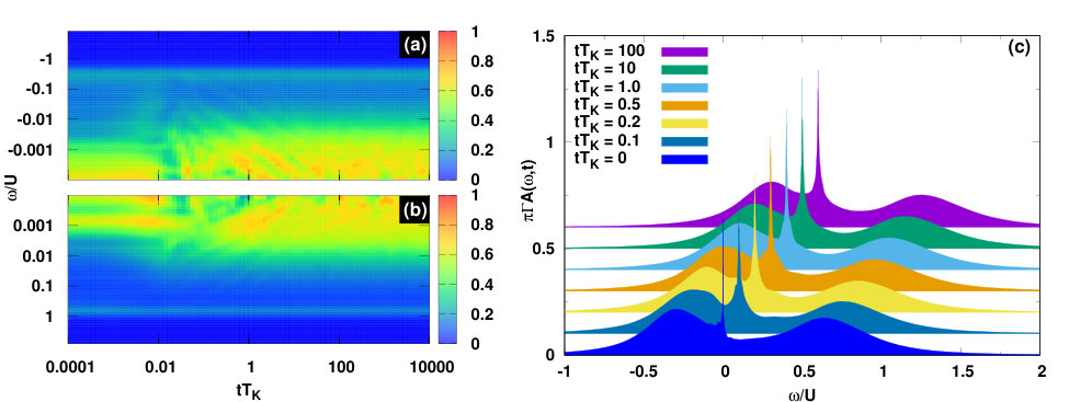 Figure 1
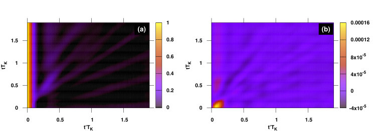 Figure 2
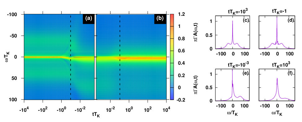 Figure 3
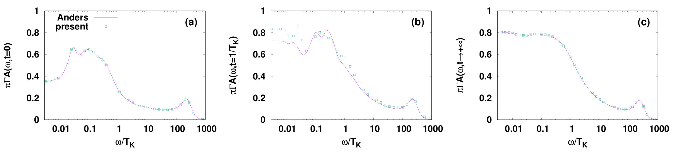 Figure 4
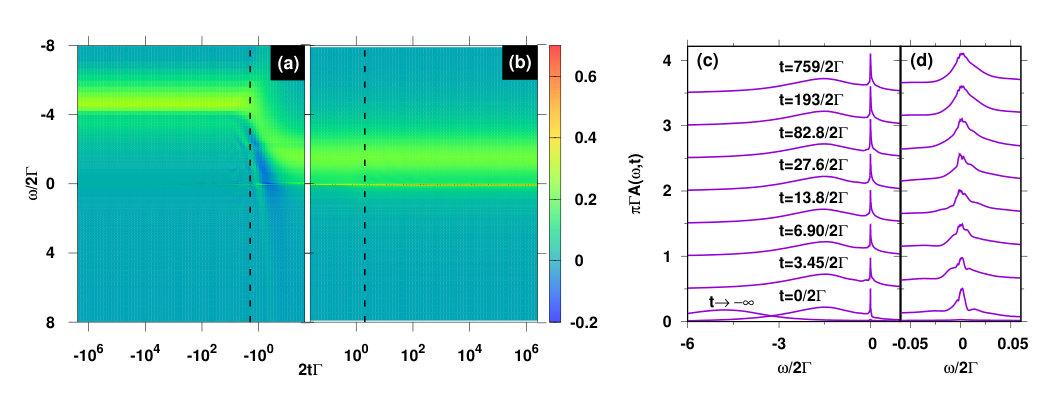 Figure 5
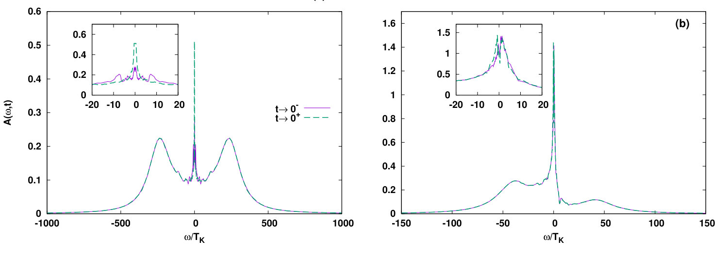 Figure 6
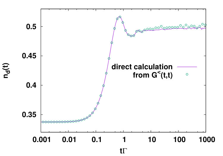 Figure 7
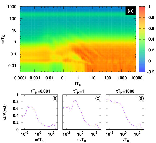 Figure 1
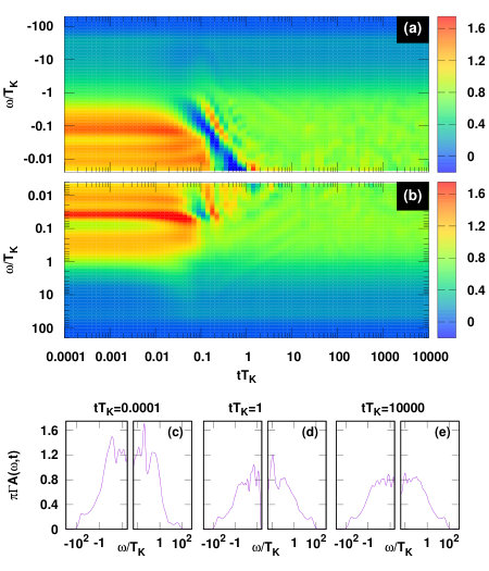 Figure 2
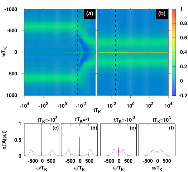 Figure 3
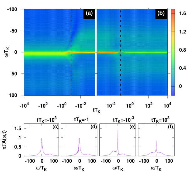 Figure 4
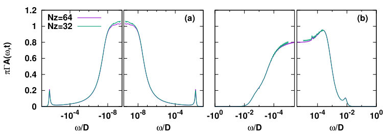 Figure 12
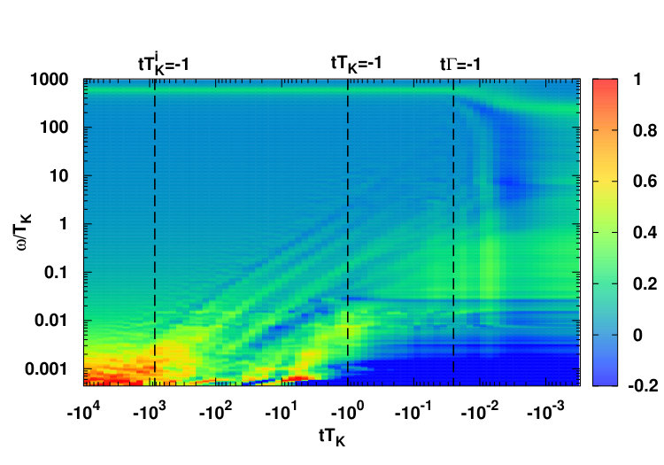 Figure 13
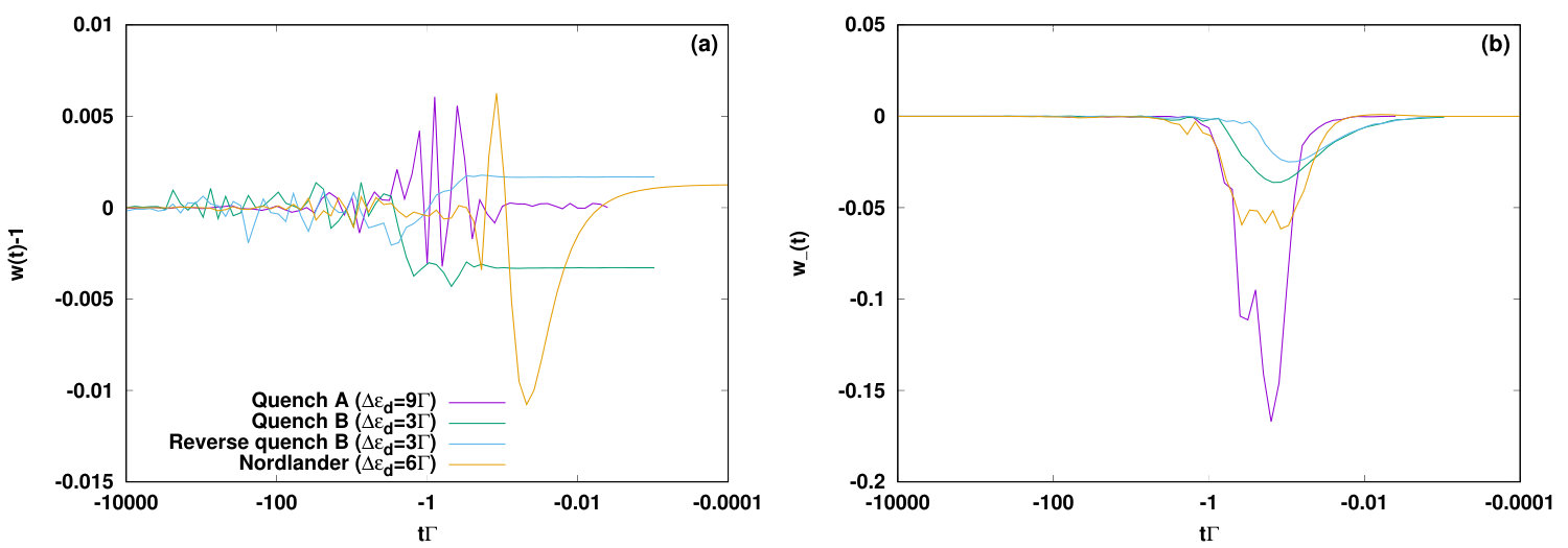 Figure 14
Peer Reviews
No public reviews on file for this paper yet. If you reviewed it on a platform where reviews are public (OpenReview, ICLR, NeurIPS, ICML), you can paste yours below so the community can read it here.
Videos
No videos yet. Explain this paper in a talk, walkthrough, or lecture? Add one.
Time evolution of the Kondo resonance in response to a quench
H. T. M. Nghiem
Peter Grünberg Institut and Institute for Advanced Simulation, Research Centre Jülich, 52425 Jülich, Germany
Advanced Institute for Science and Technology, Hanoi University of Science and Technology, 10000 Hanoi, Vietnam
T. A. Costi
Peter Grünberg Institut and Institute for Advanced Simulation, Research Centre Jülich, 52425 Jülich, Germany
Abstract
We investigate the time evolution of the Kondo resonance in response to a quench by applying the time-dependent numerical renormalization group (TDNRG) approach to the Anderson impurity model in the strong correlation limit. For this purpose, we derive within TDNRG a numerically tractable expression for the retarded two-time nonequilibrium Green function , and its associated time-dependent spectral function, , for times both before and after the quench. Quenches from both mixed valence and Kondo correlated initial states to Kondo correlated final states are considered. For both cases, we find that the Kondo resonance in the zero temperature spectral function, a preformed version of which is evident at very short times , only fully develops at very long times , where is the Kondo temperature of the final state. In contrast, the final state satellite peaks develop on a fast time scale during the time interval , where is the hybridization strength. Initial and final state spectral functions are recovered in the limits and , respectively. Our formulation of two-time nonequilibrium Green functions within TDNRG provides a first step towards using this method as an impurity solver within nonequilibrium dynamical mean field theory.
pacs:
75.20.Hr, 71.27.+a, 72.15.Qm, 73.63.Kv
Introduction.— The nonequilibrium properties of strongly correlated quantum impurity models continue to pose a major theoretical challenge. This contrasts with their equilibrium properties, which are largely well understood Hewson (1993), or can be investigated within a number of highly accurate methods, such as the numerical renormalization group method (NRG) Wilson (1975); Krishna-murthy et al. (1980); Bulla et al. (2008); Gonzalez-Buxton and Ingersent (1998), the continuous time quantum Monte Carlo (CTQMC) approach Gull et al. (2011), the density matrix renormalization group White (1992), or the Bethe ansatz method Tsvelick and Wiegmann (1983); Andrei (2013). Quantum impurity models far from equilibrium are of direct relevance to several fields of research, including charge transfer effects in low-energy ion-surface scattering Brako and Newns (1981); Kasai and Okiji (1987); Merino and Marston (1998); Langreth and Nordlander (1991); Shao et al. (1994a, b); Pamperin et al. (2015); He and Yarmoff (2010), transient and steady state effects in molecular and semiconductor quantum dots Hershfield et al. (1992); Hershfield (1993); Meir et al. (1993); Bruder and Schoeller (1994); Kretinin et al. (2011, 2012); Pletyukhov and Schoeller (2012); Scott et al. (2013); Nordlander et al. (1999); Park et al. (2002); Kogan et al. (2004); Hemingway et al. (2014); Jauho et al. (1994); Kennes et al. (2012); Cohen et al. (2014); Schmidt et al. (2008); Dorda et al. (2014); Rosch et al. (2003); Antipov et al. (2016), and also in the context of dynamical mean field theory (DMFT) of strongly correlated lattice models Metzner and Vollhardt (1989); Georges et al. (1996); Kotliar and Vollhardt (2004), as generalized to nonequilibrium Schmidt and Monien (2002); Freericks et al. (2006); Aoki et al. (2014). In the latter, further progress hinges on an accurate non-perturbative solution for the nonequilibrium Green functions of an effective quantum impurity model. Such a solution, beyond allowing time-resolved spectroscopies of correlated lattice systems within DMFT to be addressed Eckstein and Kollar (2008); Freericks et al. (2009); Perfetti et al. (2006); Loukakos et al. (2007); Iyoda and Ishihara (2014), would also be useful in understanding time-resolved scanning tunnelling microscopy of nanoscale systems Loth et al. (2010) and proposed cold atom realizations of Kondo correlated states Nishida (2013); Bauer et al. (2013); Nishida (2016); Riegger et al. (2017), which could be probed with real-time radio-frequency spectroscopy Goold et al. (2011); Knap et al. (2012); Cetina et al. (2016).
In this Letter, we use the time-dependent numerical renormalization group (TDNRG) approach Anders and Schiller (2005, 2006); Anders (2008a, b); Güttge et al. (2013); Nghiem and Costi (2014a, b) to calculate the retarded two-time Green function, , and associated spectral function, , of the Anderson impurity model in response to a quench at time , and apply this to investigate in detail the time evolution of the Kondo resonance. This topic has been addressed before within several approaches, including the non-crossing approximation Nordlander et al. (1999); Randi et al. (2017), conserving approximations Bock et al. (2016) and within CTQMC for quantum dots out of equilibrium Cohen et al. (2014). Related work on the temporal evolution of the spin-spin correlation function in the Kondo model and thermalization in the Anderson impurity model following initial state preparations has also been carried out Lobaskin and Kehrein (2005); Heyl and Kehrein (2010). Formulations of the time-dependent spectral function within TDNRG are also available Anders (2008b); Weymann et al. (2015), but only for positive times. Here, we derive expressions for the two-time Green function and spectral function which are numerically tractable at arbitrary times, including negative times. The main advantages of the TDNRG over other approaches for calculating time-dependent spectral functions is that it can access arbitrary long times () and arbitrary low temperatures and frequencies, is non-perturbative and calculates spectral functions directly on the real frequency axis. It is therefore well suited for investigating the formation in time of the exponentially narrow and low temperature Kondo resonance 111The use of a discretized Wilson chain within TDNRG results, to a small degree, in incomplete thermalization at in thermodynamic observables Anders and Schiller (2006); Rosch (2012); Nghiem and Costi (2014a); Nghiem et al. (2016), and in spectral functions Anders (2008b); Weymann et al. (2015), but it suffices for a consistent nonperturbative picture of the overall time evolution of .
*Model and quenches.—*We consider the time-dependent Anderson impurity model, , where is the energy of the local level, is the local Coulomb interaction, labels the spin, is the number operator for local electrons with spin , and is the kinetic energy of the conduction electrons with constant density of states with the half-bandwidth. We take throughout and consider two types of quench [referred to subsequently as quench (A) or quench (B)]: (A), from a symmetric Kondo regime with and a vanishingly small Kondo scale 222We use the Bethe ansatz expression valid in the symmetric Kondo limit Zlatić and Horvatić (1983); Hewson (1993). to a symmetric Kondo regime with and a larger Kondo scale , and, (B), from a mixed valence regime with to a symmetric Kondo regime with and a Kondo scale .
Spectral function .— We obtain the time-dependent spectral function via , where , with infinitesimal , is the Fourier transform of with respect to the relative time and denotes the full density matrix of the initial state Weichselbaum and von Delft (2007); Peters et al. (2006); Costi and Zlatić (2010). In the notation of Ref. Nghiem and Costi, 2014a, we find for the case of positive times 333See Supplementary Material [URL] for derivations and additional results, including Ref. Bulla et al., 2001.
[TABLE]
where , , and is the full reduced density matrix projected onto the final states Nghiem and Costi (2014a). A somewhat more complicated expression can be derived for negative times Note (3). From Eq. (1), we see that the spectral function can be calculated highly efficiently at all times and frequencies from a knowledge of , the final state matrix elements, and excitations at each shell . Our expressions for in the two time domains and recover the initial and final state spectral functions for and , respectively and satisfy the spectral sum rule exactly Note (3). Below, we shall first focus on positive times, where the main time evolution of the Kondo resonance occurs, then on negative to positive times, showing how the high energy final state features in evolve from their initial state counterparts already at negative times.
Results for positive times.— Consider quench (A), i.e., switching between symmetric Kondo regimes with . Figure 1(a) shows the overall time-dependence of the spectral function . Two structures, associated with two energy scales, are visible at all times : the satellite peak at and a structure on the scale of around the Fermi level. The former has negligible time-dependence, indicating that the satellite peak in the spectral function has already formed by time (its evolution at negative times from the initial state satellite peak at is discussed below). In contrast to this, the structure around the Fermi level has significant time-dependence at and evolves into the fully formed final state Kondo resonance only on time scales [Figs. 1(c) and 1(d)] in agreement with Ref. Nordlander et al., 1999 for the Anderson model. For , the height of the Kondo resonance at the Fermi level approaches its unitary value given by the Friedel sum rule to within [Fig. 1(d)]. The small deviation from the expected value is a result of incomplete thermalization due to the discretized Wilson chain used within TDNRG Rosch (2012); Weymann et al. (2015); Note (3). Consequently, evaluating via the self-energy Bulla et al. (1998) does not improve the Friedel sum rule further in this limit Anders (2008b). In the opposite limit, , where thermalization is not an issue, we recover the Friedel sum rule to within (discussed below). The use of a discrete Wilson chain is also the origin of the small substructures at in Figs. 1(b)-1(d), effects seen in the time evolution of other quantities, such as the local occupation, and explained in terms of the discrete Wilson chain Eidelstein et al. (2012). On shorter time scales, , states in the region , initially missing [Fig. 1(b)], are gradually filled in by a transfer of spectral weight from higher energies [Fig. 1(c)] to form the final state Kondo resonance at long times [Fig. 1(d)]. The presence of a structure on the final state Kondo scale at short times is understood as follows: the Fourier transform with respect to necessarily convolutes information about the final state at large into the spectral function at short-times Turkowski and Freericks (2005). Hence, the gross features of the spectral function, even at short times , are close to those of the final state spectral function , and far from those of the initial state spectral function. Clear signatures of the latter, such as the much narrower initial state Kondo peak, only appear at negative times.
Consider now quench (B), in which the system, is switched from the mixed valence to the symmetric Kondo regime. Figures 2(a)-(b) show the overall time-dependence of the spectral function for [Figure 2(a)] and [Figure 2(b)]. As for quench (A), two structures associated with two energy scales are again visible at all times : the satellite peaks at [Figure 2(a)] and [Figure 2(b)] and a structure on the scale of around the Fermi level [Figs. 2(a) and 2(b)]. In contrast to quench (A), the former have some non-negligible time-dependence at short positive times as can be seen in Fig. 2(c) for (), where the weight of the satellite peaks has still not equalized. This asymmetry vanishes on time scales exceeding [Figs. 2(d) and 2(e) for () and (), respectively]. The low energy structure of width , initially asymmetric and exceeding the unitary height , has significant time-dependence for and evolves into the fully developed Kondo resonance at [Figs. 2(d) and 2(e)]. The deviation from the Friedel sum rule is comparable to that for quench (A) and reflects the incomplete thermalization due to the discrete Wilson chain used within TDNRG. The discrete Wilson chain also results in the substructures at in Figs. 2(c) and 2(d) and in the small remaining asymmetry of the fully developed Kondo resonance in Fig. 2(e).
From negative to positive times.— Figures 3(a) and 3(b) show the overall time-dependence of the spectral function for negative and positive times, respectively, for quench (A), on a linear frequency scale. As for positive times [Fig. 1(a) and Fig. 3(b)], low and high energy structures are visible also for negative times [Fig. 3(a)]. Moreover, it is clear from Figs. 3(a) and 3(b) that the transition from the initial to the final state spectral function occurs on different time scales for the different structures. Consider first the high energy structures, which carry essentially all the spectral weight. Initially, these are located at as is clearly visible in Fig. 3(a) or in Fig. 3(c) for (). They cross over to their final state positions at when () [Figs. 3(a) and 3(e)], i.e., on the charge fluctuation time scale . This can also be seen in Figs. 3(d) and 3(e). This large shift in spectral weight from to in the time-range (), clearly seen in Fig. 3(a), is accompanied by small regions of negative spectral weight in this transient time range Note (3). This does not violate any exact results for time-dependent, as opposed to steady-state, spectral functions, and is observed in other systems Dirks et al. (2013); Freericks and Turkowski (2009); Jauho et al. (1994). The spectral sum rule is satisfied analytically exactly at all times and numerically within at all negative times and to higher accuracy at positive times for all quench protocols Note (3). Turning now to the low energy structure, i.e., the Kondo resonance, the use of a linear frequency scale now allows the initial state Kondo resonance at to be clearly seen in Fig. 3(a) [see also Fig. 3(c)]. This structure, of width at and satisfying the Friedel sum rule , gradually broadens and acquires a width of at short negative times Note (3), and then evolves into the fully developed Kondo resonance on positive time scales [Fig. 3(e)].
Even more interesting is the negative [Fig. 4(a)] to positive [Fig. 4(b)] time evolution of the spectral function upon quenching from the mixed valence to the symmetric Kondo regime [quench (B)]. At large negative times [Fig. 4(c)], one recovers the initial state spectral function of the mixed valence regime (with ) showing a mixed valence resonance, renormalized by many-body effects to lie close to, but just above the Fermi level and satisfying the Friedel sum rule to within Costi et al. (1996) [Figs. 4(a) and 4(c), ]. The upper satellite peak at is more clearly visible in Fig. 4(c). These peaks give rise to the final state satellite peaks at which start to form already at negative times (), i.e., on the charge fluctuation time scale , as for quench (A). While the positions of these peaks start to shift to their final state values at negative times (), their weights remain disparate [see Fig. 4(e)] and only equalize at () as clearly seen in Fig. 4(b), i.e., the formation of the high energy final state satellite peaks occurs on a fast time scale in the interval (dashed lines in Fig.4). Going into more details, we see in Figs. 4(a) and 4(c)-(e) the deconstruction of the mixed valence resonance in the time range . While this resonance carries essentially all the spectral weight at , weight is gradually transferred to , with precursor oscillations starting at () [Fig. 4(d)], to form the lower final state satellite peak at for [Fig. 4(e)] . Simultaneously, the mixed valence resonance narrows from its original width and shifts towards the Fermi level to form a low energy structure on the scale of [Fig. 4(e)]. The latter eventually evolves into the final state Kondo resonance at . The final state spectral function is recovered in the long-time limit [Fig. 4(f)].
Conclusions.— In summary, we investigated within the TDNRG the time evolution of the spectral function of the Anderson impurity model in the strong correlation limit. Quenching into a Kondo correlated final state, we showed that the Kondo resonance in the zero temperature spectral function only fully develops at very long times , although a preformed version of it is evident even at very short times . The latter can be used as a smoking gun signature of the transient build up of the Kondo resonance in future cold atom realizations of the Anderson impurity model Bauer et al. (2013). The satellite peaks evolve from their initial state values at negative times on a much faster time scale in the time-interval . Our formulation of sum rule conserving two-time nonequilibrium Green functions within TDNRG, including lesser Green functions, and their explicit dependence on both times Note (3), yields the basic information required for applications to time-dependent quantum transport Jauho et al. (1994) and constitutes a first step towards using TDNRG as an impurity solver within nonequilibrium DMFT Freericks et al. (2006); Gramsch et al. (2013); Aoki et al. (2014).
Acknowledgements.
H. T. M. N. thanks Hung T. Dang for fruitful discussions. We acknowledge support from the Deutsche Forschungsgemeinschaft via RTG 1995 and supercomputer support by the John von Neumann institute for Computing (Jülich). One of the authors (T. A. C.) acknowledges useful discussions with A. Rosch, J. K. Freericks and the hospitality of the Aspen Center for Physics, supported by the National Science Foundation under grant PHY-1607611, during completion of this work.
I Retarded two-time nonequilibrium Green function in TDNRG
We consider the retarded two-time Green function for a system undergoing a quantum quench at as described by the time-dependent Hamiltonian , with the density matrix of the initial state, represented by the full density matrix in Eq. (S18) Weichselbaum and von Delft (2007). Since , we have two cases to consider, (i), , in which case both operators and evolve with respect to , and, (ii), , in which case, either both operators evolve with respect to if , or if operator evolves with respect to , while operator evolves with respect to . While the Fourier transform with respect to the time difference yielding and hence is straightforward in case (i), in case (ii), expressions for are needed from both time domains and in order to construct and hence . Depending on the physical system considered, both positive and negative times may be of interest. Thus, in problems where the quench represents an initial state preparation, the main interest is in the evolution at following this preparation Lobaskin and Kehrein (2005). However, if the quench is considered to be a perturbation applied to the system at time , the full time evolution is of interest. This case is also required for applications to nonequilibrium dynamical field theory (DMFT)Freericks et al. (2006); Turkowski and Freericks (2005); Aoki et al. (2014). From a theoretical point of view, is also of interest to fully describe the evolution of the spectral function from its initial state value at to its final state value at .
I.1 Positive time-dependence
We first consider the case , treating in the next subsection. We have for the retarded Green function,
[TABLE]
where for fermionic/bosonic Green functions, respectively. In the notation of Ref. Nghiem and Costi, 2014a and following the approach of Anders Anders (2008), we have for the first () term of the anticommutator with
[TABLE]
where is the complete set of eliminated states in the NRG diagonalization procedure, with the first iteration at which states are eliminated and is the last NRG iteration (see Refs. Anders and Schiller (2006); Nghiem and Costi (2014a) for details). We evaluate by inserting the decomposition of unity Anders and Schiller (2006) between and ,
[TABLE]
The first term in the above expression is diagonal in the environment variables , , and runs over all states (kept and discarded) at the shell . We put in the last term to obtain
[TABLE]
Substituting (S4) into (S3) and using the NRG approximation, we have
[TABLE]
Substituting and into Eq. (S5), results in the following expression for Eq. (S2)
[TABLE]
in which is the projected full reduced density matrix known from Ref. Nghiem and Costi, 2014a. Fourier transforming the above equation with respect to gives
[TABLE]
with is a positive infinitesimal. Similarly, the second () term of the anticommutator in (S1) gives us
[TABLE]
Hence, for positive times we obtain .
In order to calculate the time-dependent spectral function from the above, one can follow Anders Anders (2008) by defining the following time-dependent density matrix
[TABLE]
Then we have the following expression for the Green’s function
[TABLE]
from which the time-dependent spectral function can be calculated. This expression of Anders Anders (2008), generalized here within the full density matrix approach, and hence valid at arbitrary temperature Nghiem and Costi (2014a), requires, however, the time-dependent reduced density matrix at each point in time, and the latter is in turn obtained via the recursion relation in Eq. (S9), resulting in a numerically highly time consuming calculation. This motivated us to develop an alternative and numerically more tractable expression for the retarded two-time Green function, to which we now turn.
A different and numerically more feasible expression for than the expression above, can be obtained if we go back to Eq. (S5) and substitute this into Eq. (S2),
[TABLE]
The first term in this expression is simply
[TABLE]
and the second term can be rearranged as follows
[TABLE]
Combining the above two terms, we have
[TABLE]
in which and all the other matrix elements are known quantities. Together with the second term () in the anticommutator,
[TABLE]
we have the retarded Green’s function as follows
[TABLE]
This expression is useful for the non-equilibrium DMFT, which requires the dynamical fields expressed in terms of two-time Green functions Freericks et al. (2006); Gramsch et al. (2013); Aoki et al. (2014). Fourier transforming with respect to the time difference gives
[TABLE]
which together with results in a time-dependent spectral function that can be evaluated at all times in a numerically highly efficient manner: only the time-independent projected density matrix together with the NRG excitations and matrix elements are required to evaluate at all positive times. While the above expression looks deceptively similar to the first term in Anders expression for the positive time Green function in Eq. (S10), this is not the case [note the different sum in Eq. (S17) as compared to the sum in the first term of Eq. (S10)]. It includes also the second term in Eq. (S10), involving , but within a different approximation that follows from the second line of Eq. (S14). In this way, the recursive evaluation of a reduced density matrix depending explicitly on time is circumvented in our expression, making it numerically tractable. A similar expression to Eq. (S17) has been derived for initial state density matrices corresponding to either pure states, such as the ground state, or to decoupled initial states ( in the Anderson model) with or without excitations in the bath and used to study thermalization in the Anderson model following such an initial state preparation Weymann et al. (2015).
As a check on Eq. (S17), we can verify that it reduces to the equilibrium retarded Green function in the case that (vanishing quench size). In this limit, using the definition of the full density matrix of the initial stateWeichselbaum and von Delft (2007),
[TABLE]
and of the reduced full density matrix in Refs. Costi and Zlatić, 2010; Nghiem and Costi, 2014a, we have
[TABLE]
Substituting this expression into Eq. (S17) for , we obtain the following time-independent expression
[TABLE]
which is identical to the expression in the equilibrium case Weichselbaum and von Delft (2007); Costi and Zlatić (2010); Nghiem and Costi (2014a).
It is interesting to compare the spectral function obtained from our Eq. (S17) with that of Anders obtained from Eq. (S10). For this purpose, we consider quench (A) of the main text and three representative times: , , and . From Figs. S1(a) and S1(c) we see that both expressions give the same results at and , while at finite times small differences arise for [see Fig. S1(b)]. As we discussed in connection with Eq. (S10) above the main advantage of our new expression Eq. (S17), is that it can be evaluated numerically very efficiently. By contrast, to date, no results at finite times have been published using Eq. (S10) and only results for infinite times have been published Anders (2008).
I.2 Negative time-dependence ()
At negative times , we can have before or after the quench. When or , we have
[TABLE]
which is -independent, and just corresponds to the equilibrium propagator of the initial state Hamiltonian (as long as ). While for or , we have
[TABLE]
In general, then, we have for the retarded Green function at
[TABLE]
For the first part ( term) of the anticommutator at we have
[TABLE]
Next, we consider , which with Eq. (S18) becomes
[TABLE]
In this sum, only the parts with are finite, and we obtain
[TABLE]
with as in Ref. Nghiem and Costi, 2014a. Substituting the above into Eq. (S23) we obtain
[TABLE]
Similarly, the first part ( term) of the anticommutator for is given by
[TABLE]
where (i.e., the tilde signifies that the time evolution operators apply to the composite operator ). We decompose the above sum into three parts corresponding to , , and , then simplify them as follows
[TABLE]
Substituting into the above equation, we have
[TABLE]
The second part ( term) of the anticommutators for the two parts at and , denoted by and , respectively, can be derived in a similar way and combining all terms gives the expression for the two-time Green function at . Fourier transforming with respect to the time difference results in the following expression for the spectral function at
[TABLE]
From this expression, we easily see that recovers the initial state Green function. While from the starting definition, we have equal to , in the approximate expressions above this is no longer guaranteed as a consequence of the NRG approximation and the different derivations for . Figures S2(a)-S2(b) show the spectral functions at and and quantify the size of the discontinuity at . While the spectral functions for match to high accuracy at high frequencies for both quench (A) [Fig. S2(a)] and quench (B) [Fig. S2(b)] of the main text, there is a mismatch at low frequencies.
In Fig. S3 we show the negative time spectral function for quench (A) of the main text using logarithmic axes for both time (in units of the initial state Kondo scale ) and frequency, (in units of the final state Kondo scale ). The data is the same as the positive frequency data in Fig. 3(a) of the main text, but the use of a logarithmic frequency axis now makes clearer the statement made there concerning the structure around the Fermi level, that “this structure, of width at and satisfying the Friedel sum rule , gradually broadens and acquires a width of at short negative times …”. In addition, Fig. S3 shows that the low energy structure on a scale at short negative times is formed by drawing spectral weight from both the initial state Kondo resonance (diagonal stripes at ), and also from the satellite peaks (starting at ). As for short positive times [Fig. 1(a) of the main text], the “preformed” Kondo resonance at short negative times () is seen to have missing states in the vicinity () of the Fermi level. Finally, notice that the relevant time scale for the “devolution” of the initial state Kondo resonance at is .
I.3 Numerical evaluation of
I.3.1 Positive time spectral function
We first consider the evaluation of the spectral function for positive times. From (S17), we have for
[TABLE]
where . The first contribution,
[TABLE]
is evaluated in the usual way by replacing by the logarithmic Gaussian and summing over the excitations Bulla et al. (2001, 2008).
In order to evaluate the second contribution above, we define the auxiliary function via
[TABLE]
and evaluate this in the usual way. Taking it’s principle value integral then gives the second contribution to the spectral function:
[TABLE]
To summarize,
[TABLE]
I.3.2 Negative time spectral function
We now consider the evaluation of for negative times starting from the expression for the retarded Green function in Eq. (S30). This is a sum of two terms , with
[TABLE]
where . Correspondingly, the spectral function is also written as a sum of two parts . Consider first , for finite , is regular, having no poles on the real axis, then is evaluated directly
[TABLE]
with a finite and where is the number of bath realizations in the averaging procedure.
For consistency, we also evaluate in Eq. (S36) with the same Lorentzian broadening and thereby obtain and thus .
I.4 Spectral sum rule
The spectral weight sum rule with is exactly satisfied for all positive times within our expression Eq. (S17) and the same holds true for Eq. (S10) (see Ref. Anders, 2008). Here, we prove that it is exactly satisfied also for all negative times. With defined by Eq. (S30), we need to evaluate the following terms
[TABLE]
with a positive infinitesimal. Defining and , we have
[TABLE]
where use was made of and (). Using Eqs. (S40-S41) and Eq. (S30), we have
[TABLE]
Therefore the sum rule is proved at . The sum rule also holds for , as can be seen by noting that the last integrals contributing to and return [math] in this case.
The numerically evaluated negative-time spectral function also satisfies this sum rule to within for all quench protocols and all negative times, as shown in Fig. S4(a). In Fig. S4(b) we show with if and if , i.e., the contribution to the total weight coming from regions of negative spectral density. Regions of negative spectral weight appear for transient times in many other systems Dirks et al. (2013); Jauho et al. (1994); Freericks and Turkowski (2009), while in steady state limits the spectral function is positive definite within canonical density matrix approaches. We see that both and the error in the sum rule are both largest in the time region where the major part of the spectral weight (located in the satellite peaks) is being rearranged from to . The maximum size of correlates with the quench size , and reaches up to for the largest quench (A) in Fig. S4(b).
I.5 Friedel sum rule, thermalization and discretization effects
The TDNRG replaces the continuum conduction electron bath in the Anderson model by a logarithmically discretized bath whose tight binding representation in energy space (the so called Wilson chain) is given by with for and where is the discretization parameter. The continuum limit corresponds to , which is not possible to take numerically within the iterative NRG diagonalization scheme due to the increasing slow convergence in this limit. The effect of using such a discrete Wilson chain on the time evolution of physical quantities in response to a quench is twofold: (i), incomplete thermalization at long times after the quench due to the fact that a Wilson chain (even in the limit ) cannot act as a proper heat bath Rosch (2012) (see also Refs. Anders and Schiller, 2006; Nghiem and Costi, 2014a, b; Weymann et al., 2015) and ,(ii), additional real features appear in the time evolution, due to the logarithmic discretization of the bath. We address these two effects in turn.
Incomplete thermalization in the long time limit is reflected in deviations of observables from their expected values in the final state. These deviations can be reduced by decreasing , as shown in Ref. Nghiem and Costi, 2014a for the case of the local occupation in the Anderson model, where was found to approach its expected value more closely upon decreasing towards . In the present context of spectral functions, incomplete thermalization is reflected in a deviation of from the continuum result , where is the occupation number in the final state. However, this deviation is not an error of the TDNRG but is expected because of (i). The Friedel sum rule (FSR) only holds for equilibrium states. In the infinite past, where thermalization issues play no role, and one achieves the equilibrium state at , the FSR is satisfied to within a for all quenches studied, which is comparable to the accuracy achievable in equilibrium NRG calculations Costi et al. (1996) (the spectra for large negative in Fig.3(c) and Fig.4(c) of the main text). This demonstrates that the deviation in the value of is not an error of the TDNRG but is the correct result for the Wilson chain used.
We note, furthermore, that other approaches to time dependent spectral densities, such as the non-crossing approximation Nordlander et al. (1999) suffer, even for equilibrium spectral densities, from much larger errors in the Friedel sum rule (see Table I in Ref. Costi et al., 1996), and still other methods Bock et al. (2016) can result in errors which exceed despite the use of a continuum bath. In the latter approaches the deviations from the Friedel sum rule represent real errors in the underlying methods, whereas in the TDNRG, the deviation observed is that expected from using a logarithmically discretized chain.
The second effect of using a Wilson chain is that additional features appear in the time evolution of physical observables that would be absent for a continuum bath. Examples are the small oscillations seen in Figs .1 and 2 of the main text at low energies . Physically, these oscillations, or ”substructures” result from the highly nonequilibrium situation created by the quench: following the quench, the local change in energy has to be transported by electrons propagating outwards in the process of thermalization. These electrons are reflected off the different sites () of the inhomogeneous Wilson chain (with hoppings ) arriving back at the impurity site where they interfere at specific times to give additional features in the time evolution of local quantities (such as in ). This was originally explained in great detail by Eidelstein et al. in Ref. Eidelstein et al., 2012 for observables like the occupation number . These authors also showed a comparison between using TDNRG and using exact diagonalization for a noninteracting resonant level model, both calculated using the same Wilson chain. The additional features in the time evolution of , not present in the continuum model, were identified as real effects and not as being due to errors or unphysical features of the TDNRG method. Thus, the features seen in Figs.1 and 2 of the main text at low energies have their origin in the logarithmically discretized bath. In the remote past, before the quench is able to act, such features are expected to be absent. In support of this interpretation, we therefore show on a logarithmic scale the spectral function in the distant past in Figs. S5(a)-S5b, which indeed show the absence of all “substructures”. This is to be compared with the presence of such ”substructures” at finite and long positive times [Figs. 1(b)-1(d) and Fig. 2(c)-2(e) in the main text]. Finally, we mention that since the limit is not feasible within NRG, a simpler approach that is useful to obtain results closer to those of the continuum limit is the averaging of time-dependent quantities over realizations of the bath Anders and Schiller (2006).
II Additional results
Our derivation for the non-equilibrium two-time retarded Green function at both positive and negative times can be used to derive expressions for the other commonly used Green functions in many-body theory, including lesser (and greater) Green functions, and can be used for arbitrary quenches. In the next subsections, we show the results for the cases of the reverse of quench (B) in the main text, i.e. quenching from a symmetric Kondo into a mixed valence regime, a finite temperature quench as in Nordlander et al. Nordlander et al. (1999), and a hybridization quench in which the coupling is switched on at time . We also show results for the lesser Green function, which together with the retarded Green function constitute the basic ingredients for many applications, e.g., to transient and non-equilibrium transport through correlated quantum dots Hershfield et al. (1992); Meir et al. (1993); Jauho et al. (1994). In Sec. II.5, we show the explicit two-time dependence of the retarded Green function, a basic ingredient in nonequilibrium DMFT applications Freericks et al. (2006).
II.1 Symmetric Kondo to mixed valence [reverse of quench (B)]
In this subsection, we show the time-dependent spectral functions for the case of the reverse of quench (B) in the main text. i.e., from the symmetric Kondo to the mixed valence regime. We see in Fig. S6 how the spectral function evolves from the spectral function of the initial state at [Fig. S6(c) for ()], with the Friedel sum rule satisfied to within a few in this limit, to its value in the long-time limit with a mixed valence peak close to the Fermi level and a satellite peak at above the Fermi level [Fig. S6(f) for ()]. Similar to the other cases in the main text, the initial state satellite peaks at rapidly relocate at [dashed line in Fig. S6(a)] with spectral weight being shifted to form the upper satellite peak and the mixed valence resonance, a process which essentially has completed by [dashed line in Fig. S6(b)]. The weights of these peaks weights are also close to those of the final state for . The central peak which represents the Kondo resonance at also varies strongly at , and evolves into the mixed valence peak by time .
II.2 Nordlander quench (finite temperature)
In Ref. Nordlander et al., 1999 a quench is made within the Anderson model via a level shift with () and (). This corresponds to a quench from one asymmetric Kondo regime to another with disparate Kondo scales; in contrast we previously investigated quenches in which one of the states was in a symmetric Kondo regime whereas the other was in an mixed valence regime. The quench in Ref. Nordlander et al., 1999 also differs from those studied so far since it is at a finite temperature such that . Thus, initially the Kondo resonance is strongly temperature suppressed whereas in the final state it is only moderately suppressed by temperature. This quench can therefore serve to illustrate the application of our TDNRG formalism for time dependent spectral functions to finite temperatures.
In figure S7, we show the time-dependent spectral function from negative to positive times. The calculations were carried out for to simulate the case. We therefore observe only the satellite peak below the Fermi level in the negative frequency range, both in the initial and final states. Similar to the other calculations, the satellite peak rapidly relocates at from to as shown in Fig. S7 (a). At the same time, the spectral function develops small regions of negative spectral weight, with the total sum-rule remaining satisfied to within as shown in Fig. S4 (a). The central peak at is absent at since the calculation is at finite temperature . Since the temperature is finite and comparable to the final state Kondo scale, the Kondo resonance does not fully develop at long times [Fig. S7(b) and S7(c)] with reaching only about of its value. This is better seen in Fig. S7(d), which shows a close up of the low frequency region around the Fermi level. Nevertheless, despite the finite temperature, one sees the build up of the Kondo resonance at .
II.3 Hybridization quench
In this subsection, we show the time-dependent spectral functions for the case of a hybridization quench as in Ref. Weymann et al., 2015, where the hybridization between the impurity and the conduction electrons, initially turned off at , is suddenly turned on at . In figure S8 (a)-(b), we see that for this quench also, low and high energy features are present at all times. The high energy features correspond to the final state satellite peaks at and , whereas the low energy feature of width on the scale of the final state Kondo temperature represents the Kondo resonance. While the former have little temperature dependence at all , as in Weymann et al. Weymann et al. (2015), the latter has significant time dependence, developing fully only at [Fig. S8(a)] with weight drawn in from higher energies in the process. Notice that this low energy peak appears even at , which is different from Weymann et al,Weymann et al. (2015) since the broadening parameter is set to be time-independent in our calculation, while it is time-dependent (and large of order at ) in Weymann et al. Weymann et al. (2015) . While the strong time dependence of the Kondo resonance can be seen on a logarithmic frequency scale from Fig. S8(a), it is barely discernible on the linear frequency scale of Fig. S8(b).
II.4 Lesser Green functions
We consider explicitly the lesser Green function for the local level in the Anderson impurity model, defined by
[TABLE]
For equal times (),
[TABLE]
i.e., , so the lesser Green function at equal times gives the time evolution of the local occupation number. Following the derivation for the retarded Green function in Sec. I, we similarly obtain the following expression for the lesser Green function
[TABLE]
with and . The time evolution of the occupation number calculated from this expression by setting can be compared with that calculated directly from the thermodynamic observable Nghiem and Costi (2014a). The two results, shown in Fig. S9, match perfectly at short times and differ slightly on longer time scales (). This small difference arises because the NRG approximation enters differently in the expressions for thermodynamic and dynamic quantities.
II.5 Retarded Green function: explicit dependence on times
From Eq. (S17), we can directly evaluate the dependence of the retarded Green function on its two time arguments. This is shown for the imaginary and real parts in Figs. S10(a)-S10(b) versus the time difference and time . At equal times we see from Fig. S10(a) that for all , recovering the canonical anticommutation relation for fermions, ande hence the spectral sum rule for . Non-equilibrium DMFT Freericks et al. (2006); Schmidt and Monien (2002); Gramsch et al. (2013); Aoki et al. (2014) requires impurity Green functions in real time, and the ability to calculate these within TDNRG, which we here demonstrated, is a useful first step for future applications to the former.
References
- Weichselbaum and von Delft (2007) A. Weichselbaum and J. von Delft, Phys. Rev. Lett. 99, 076402 (2007).
- Anders (2008) F. B. Anders, Journal of Physics-Condensed Matter 20, 195216 (2008).
- Nordlander et al. (1999) P. Nordlander, M. Pustilnik, Y. Meir, N. S. Wingreen, and D. C. Langreth, Phys. Rev. Lett. 83, 808 (1999).
- Weymann et al. (2015) I. Weymann, J. von Delft, and A. Weichselbaum, Phys. Rev. B 92, 155435 (2015).
- Lobaskin and Kehrein (2005) D. Lobaskin and S. Kehrein, Phys. Rev. B 71, 193303 (2005).
- Freericks et al. (2006) J. K. Freericks, V. M. Turkowski, and V. Zlatić, Phys. Rev. Lett. 97, 266408 (2006).
- Turkowski and Freericks (2005) V. Turkowski and J. K. Freericks, Phys. Rev. B 71, 085104 (2005).
- Aoki et al. (2014) H. Aoki, N. Tsuji, M. Eckstein, M. Kollar, T. Oka, and P. Werner, Rev. Mod. Phys. 86, 779 (2014).
- Nghiem and Costi (2014a) H. T. M. Nghiem and T. A. Costi, Phys. Rev. B 89, 075118 (2014a).
- Anders and Schiller (2006) F. B. Anders and A. Schiller, Phys. Rev. B 74, 245113 (2006).
- Gramsch et al. (2013) C. Gramsch, K. Balzer, M. Eckstein, and M. Kollar, Phys. Rev. B 88, 235106 (2013).
- Costi and Zlatić (2010) T. A. Costi and V. Zlatić, Phys. Rev. B 81, 235127 (2010).
- Bulla et al. (2001) R. Bulla, T. A. Costi, and D. Vollhardt, Phys. Rev. B 64, 045103 (2001).
- Bulla et al. (2008) R. Bulla, T. A. Costi, and T. Pruschke, Rev. Mod. Phys. 80, 395 (2008).
- Dirks et al. (2013) A. Dirks, M. Eckstein, T. Pruschke, and P. Werner, Phys. Rev. E 87, 023305 (2013).
- Jauho et al. (1994) A.-P. Jauho, N. S. Wingreen, and Y. Meir, Phys. Rev. B 50, 5528 (1994).
- Freericks and Turkowski (2009) J. K. Freericks and V. Turkowski, Phys. Rev. B 80, 115119 (2009).
- Rosch (2012) A. Rosch, The European Physical Journal B-Condensed Matter and Complex Systems 85, 1 (2012).
- Nghiem and Costi (2014b) H. T. M. Nghiem and T. A. Costi, Phys. Rev. B 90, 035129 (2014b).
- Costi et al. (1996) T. A. Costi, J. Kroha, and P. Wölfle, Phys. Rev. B 53, 1850 (1996).
- Bock et al. (2016) S. Bock, A. Liluashvili, and T. Gasenzer, Phys. Rev. B 94, 045108 (2016).
- Eidelstein et al. (2012) E. Eidelstein, A. Schiller, F. Güttge, and F. B. Anders, Phys. Rev. B 85, 075118 (2012).
- Hershfield et al. (1992) S. Hershfield, J. H. Davies, and J. W. Wilkins, Phys. Rev. B 46, 7046 (1992).
- Meir et al. (1993) Y. Meir, N. S. Wingreen, and P. A. Lee, Phys. Rev. Lett. 70, 2601 (1993).
- Schmidt and Monien (2002) P. Schmidt and H. Monien, eprint arXiv:cond-mat/0202046 (2002), cond-mat/0202046 .
- Cohen et al. (2014) G. Cohen, E. Gull, D. R. Reichman, and A. J. Millis, Phys. Rev. Lett. 112, 146802 (2014).
The reference list from the paper itself. Each links out to its DOI / PubMed record.
- 1Hewson (1993) A. C. Hewson, Phys. Rev. Lett. 70 , 4007 (1993) . · doi ↗
- 2Wilson (1975) K. G. Wilson, Rev. Mod. Phys. 47 , 773 (1975) . · doi ↗
- 3Krishna-murthy et al. (1980) H. R. Krishna-murthy, J. W. Wilkins, and K. G. Wilson, Phys. Rev. B 21 , 1003 (1980) . · doi ↗
- 4Bulla et al. (2008) R. Bulla, T. A. Costi, and T. Pruschke, Rev. Mod. Phys. 80 , 395 (2008) . · doi ↗
- 5Gonzalez-Buxton and Ingersent (1998) C. Gonzalez-Buxton and K. Ingersent, Phys. Rev. B 57 , 14254 (1998) . · doi ↗
- 6Gull et al. (2011) E. Gull, A. J. Millis, A. I. Lichtenstein, A. N. Rubtsov, M. Troyer, and P. Werner, Rev. Mod. Phys. 83 , 349 (2011) . · doi ↗
- 7White (1992) S. R. White, Phys. Rev. Lett. 69 , 2863 (1992) . · doi ↗
- 8Tsvelick and Wiegmann (1983) A. M. Tsvelick and P. B. Wiegmann, Advances in Physics 32 , 453 (1983) . · doi ↗