Statistical Decoding
Thomas Debris-Alazard, Jean-Pierre Tillich

TL;DR
This paper analyzes statistical decoding, a randomized approach for code-based cryptography, providing its asymptotic complexity, efficient computation methods, and bounds, showing it cannot outperform Prange's algorithm at the Gilbert-Varshamov bound.
Contribution
It offers the first detailed complexity analysis of statistical decoding, introduces efficient computation techniques, and establishes lower bounds on its performance.
Findings
Provides asymptotic complexity of statistical decoding.
Develops efficient methods for computing parity-check equations.
Shows statistical decoding cannot outperform Prange's algorithm at the Gilbert-Varshamov bound.
Abstract
The security of code-based cryptography relies primarily on the hardness of generic decoding with linear codes. The best generic decoding algorithms are all improvements of an old algorithm due to Prange: they are known under the name of information set decoding techniques (ISD). A while ago a generic decoding algorithm which does not belong to this family was proposed: statistical decoding. It is a randomized algorithm that requires the computation of a large set of parity-check equations of moderate weight. We solve here several open problems related to this decoding algorithm. We give in particular the asymptotic complexity of this algorithm, give a rather efficient way of computing the parity-check equations needed for it inspired by ISD techniques and give a lower bound on its complexity showing that when it comes to decoding on the Gilbert-Varshamov bound it can never be better…
Click any figure to enlarge with its caption.
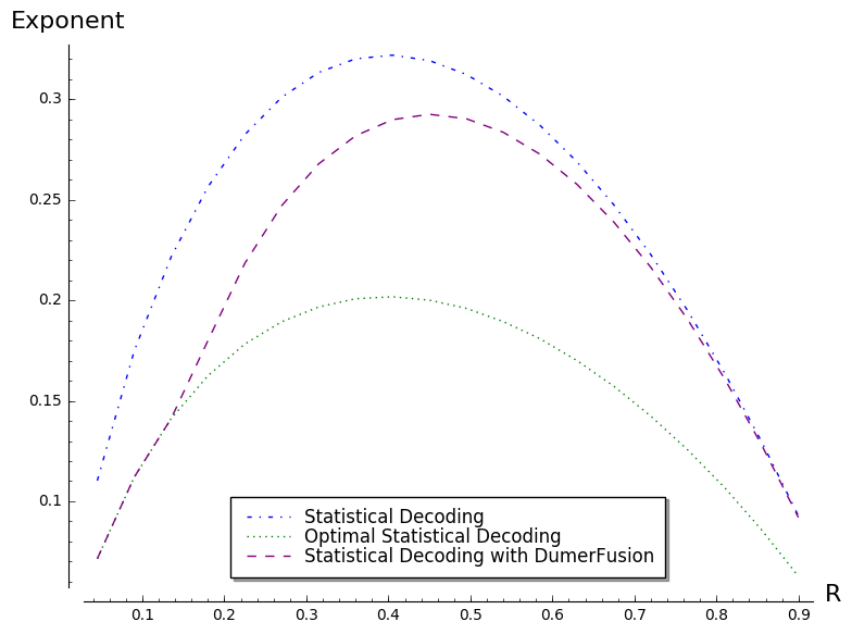 Figure 1
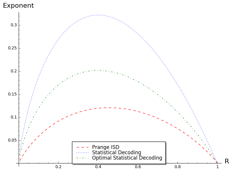 Figure 2
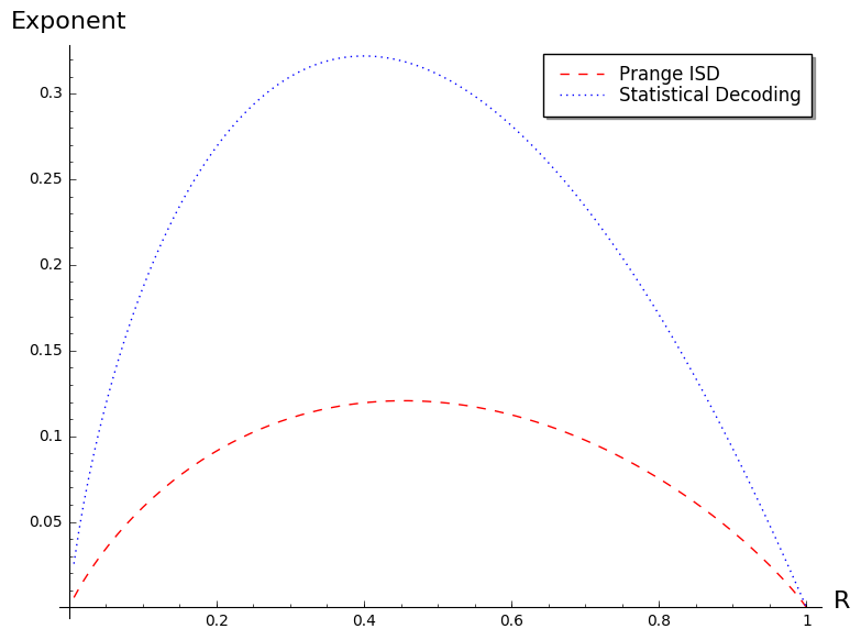 Figure 3
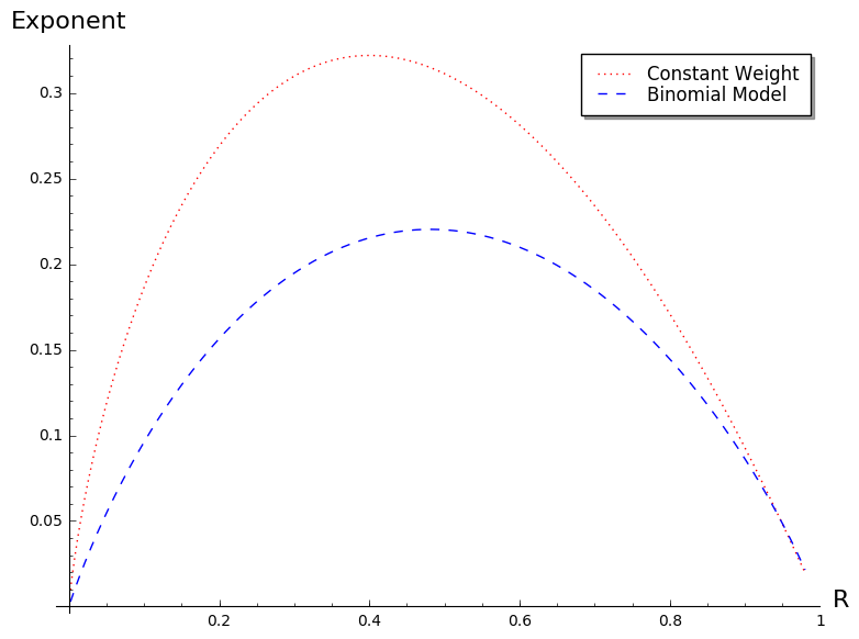 Figure 4
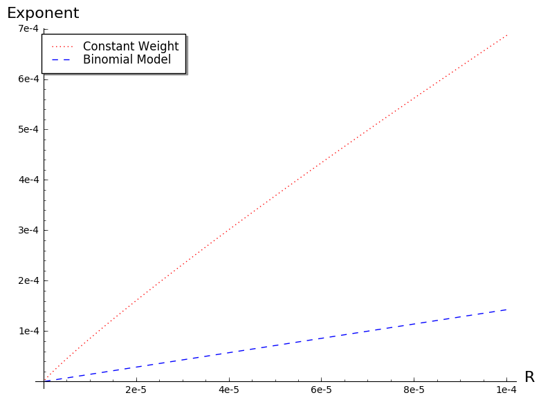 Figure 5
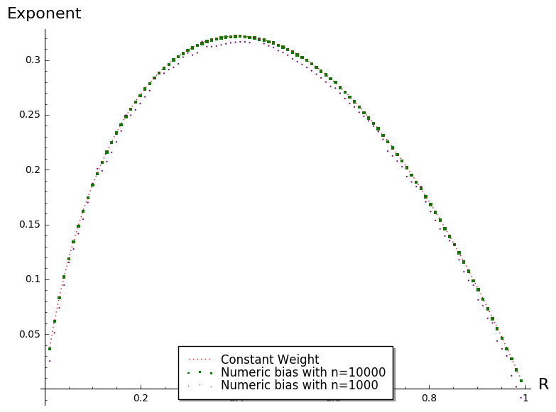 Figure 6
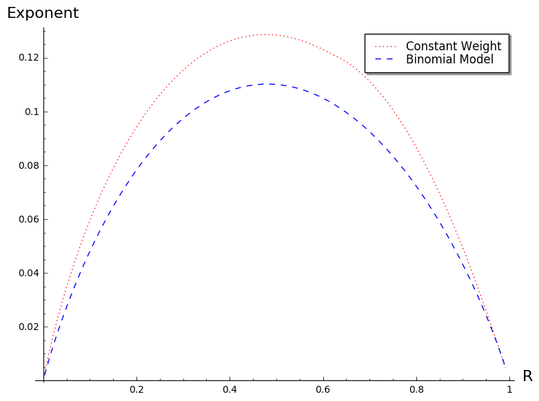 Figure 7
Peer Reviews
No public reviews on file for this paper yet. If you reviewed it on a platform where reviews are public (OpenReview, ICLR, NeurIPS, ICML), you can paste yours below so the community can read it here.
Videos
No videos yet. Explain this paper in a talk, walkthrough, or lecture? Add one.
Statistical Decoding
Thomas Debris-Alazard ∗
Jean-Pierre Tillich 111Inria, SECRET Project, 2 Rue Simone Iff 75012 Paris Cedex, France, Email: {thomas.debris,jean-pierre.tillich}@inria.fr. Part of this work was supported by the Commission of the European Communities through the Horizon 2020 program under project number 645622 PQCRYPTO.
Abstract
The security of code-based cryptography relies primarily on the hardness of generic decoding with linear codes. The best generic decoding algorithms are all improvements of an old algorithm due to Prange: they are known under the name of information set decoding techniques (ISD). A while ago a generic decoding algorithm which does not belong to this family was proposed: statistical decoding. It is a randomized algorithm that requires the computation of a large set of parity-check equations of moderate weight. We solve here several open problems related to this decoding algorithm. We give in particular the asymptotic complexity of this algorithm, give a rather efficient way of computing the parity-check equations needed for it inspired by ISD techniques and give a lower bound on its complexity showing that when it comes to decoding on the Gilbert-Varshamov bound it can never be better than Prange’s algorithm.
1 Introduction
Code-based cryptography relies crucially on the hardness of decoding generic linear codes. This problem has been studied for a long time and despite many efforts on this issue [Pra62, Ste88, Dum91, Bar97, MMT11, BJMM12, MO15] the best algorithms for solving this problem [BJMM12, MO15] are exponential in the number of errors that have to be corrected: correcting errors in a binary linear code of length has with the aforementioned algorithms a cost of where is a constant depending of the code rate and the algorithm. All the efforts that have been spent on this problem have only managed to decrease slightly this exponent . Let us emphasize that this exponent is the key for estimating the security level of any code-based cryptosystem.
All the aforementioned algorithms can be viewed as a refinement of the original Prange algorithm [Pra62] and are actually all referred to as ISD algorithms. There is however an algorithm that does not rely at all on Prange’s idea and does not belong to the ISD family: statistical decoding proposed first by Al Jabri in [Jab01] and improved a little bit by Overbeck in [Ove06]. Later on, [FKI07] proposed an iterative version of this algorithm. It is essentially a two-stage algorithm, the first step consisting in computing an exponentially large number of parity-check equations of the smallest possible weight , and then from these parity-check equations the error is recovered by some kind of majority voting based on these parity-check equations.
However, even if the study made by R. Overbeck in [Ove06] lead to the conclusion that this algorithm did not allow better attacks on the cryptosystems he considered, he did not propose an asymptotic formula of its complexity that would have allowed to conduct a systematic study of the performances of this algorithm. Such an asymptotic formula has been proposed in [FKI07] through a simplified analysis of statistical decoding, but as we will see this analysis does not capture accurately the complexity of statistical decoding. Moreover both papers did not assess in general the complexity of the first step of the algorithm which consists in computing a large set of parity-check equations of moderate weight.
The primary purpose of this paper is to clarify this matter by giving three results. First, we give a rigorous asymptotic study of the exponent of statistical decoding by relying on asymptotic formulas for Krawtchouk polynomials [IS98]. The number of equations which are needed for this method turns out to be remarkably simple for a large set of parameters. In Theorem 2 we prove that the number of parity check equations of weight that are needed in a code of length to decode errors is of order (when we ignore polynomial factors) and this as soon as . For instance, when we consider the hardest instances of the decoding problem which correspond to the case where the number of errors is equal to the Gilbert-Varshamov bound, then essentially our results indicate that we have to take all possible parity-checks of a given weight (when the code is assumed to be random) to perform statistical decoding. This asymptotic study also allows to conclude that the modeling of iterative statistical decoding made in [FKI07] is too optimistic. Second, inspired by ISD techniques, we propose a rather efficient method for computing a huge set of parity-check equations of rather low weight. Finally, we give a lower bound on the complexity of this algorithm that shows that it can not improve upon Prange’s algorithm for the hardest instances of decoding.
This lower bound follows by observing that the number of the parity-check equations of weight that are needed for the second step of the algorithm is clearly a lower-bound on the complexity of statistical decoding. What we actually prove in the last part of the paper is that irrelevant of the way we obtain these parity-check equations in the first step, the lower bound on the complexity of statistical decoding coming from the infimum of these ’s is always larger than the complexity of the Prange algorithm for the hardest instances of decoding.
2 Notation
As our study will be asymptotic, we neglect polynomial factors and use the following notation:
Notation 1**.**
Let , we write iff there exists a polynomial such that .
Moreover, we will often use the classical result where denotes the binary entropy. We will also have to deal with complex numbers and follow the convention of the article [IS98] we use here: i is the imaginary unit satisfying the equation , is the real part of the complex number and we choose the branch of the complex logarithm with
[TABLE]
and .
3 Statistical Decoding
In the whole paper we consider the computational decoding problem which we define as follows:
Problem 1**.**
Given a binary linear code of length of rate , a word at distance from the code, find a codeword such that where denotes the Hamming distance.
Generally we will specify the code by an arbitrary generator matrix and we will denote by CSD a specific instance of this problem. We will be interested as is standard in cryptography in the case where is supposed to be random.
The idea behind statistical decoding may be described as follows. We first compute a very large set of parity-check equations of some weight and compute all scalar products (scalar product is modulo ) for . It turns out that if we consider only the parity-checks involving a given code position the scalar products have a probability of being equal to which depends whether there is an error in this position or not. Therefore counting the number of times when allows to recover the error in this position.
Let us analyze now this algorithm more precisely. To make this analysis tractable we will need to make a few simplifying assumptions. The first one we make is the same as the one made by R. Overbeck in [Ove06], namely that
Assumption 1**.**
The distribution of the ’s when is drawn uniformly at random from the dual codewords of weight is approximated by the distribution of when is drawn uniformly at random among the words of weight .
A much simpler model is given in [FKI07] and is based on modeling the distribution of the ’s as the distribution of where the coordinates of are i.i.d. and distributed as a Bernoulli variable of parameter . This presents the advantage of making the analysis of statistical decoding much simpler and allows to analyze more refined versions of statistical decoding. However as we will show, this is an oversimplification and leads to an over-optimistic estimation of the complexity of statistical decoding. The following notation will be useful.
Notation 2**.**
denotes the set of binary of words of length of weight ;
;
;
;
means that follows a Bernoulli law of parameter ;
means we pick uniformly at random in .
3.1 Bias in the parity-check sum distribution
We start the analysis of statistical decoding by computing the following probabilities which approximate the true probabilities we are interested in (which correspond to choosing uniformly at random in and not in ) under Assumption 1
[TABLE]
[TABLE]
These probabilities are readily seen to be equal to
[TABLE]
[TABLE]
They are independent of the error and the position . So, in the following we will use the notation and . We will define the biases and of statistical decoding by
[TABLE]
It will turn out, and this is essential, that . We can use these biases “as a distinguisher”. They are at the heart of statistical decoding. Statistical decoding is nothing but a statistical hypothesis testing algorithm distinguishing between two hypotheses :
[TABLE]
based on computing the random variable for uniform and independent draws of vectors in :
[TABLE]
We have according to . So the expectation of is given under by:
[TABLE]
We point out that we have regardless of the term . In order to apply the following proposition, we make the following assumption:
Assumption 2**.**
are independent variables.
Proposition 1** (Chernoff’s Bound).**
Let , i.i.d and we set . Then,
[TABLE]
Consequences: Under , we have
[TABLE]
To take our decision we proceed as follows: if where
[TABLE]
we choose and if not. For the cases of interest to us (namely and linear in ) the bias is an exponentially small function of the codelength and it is obviously enough to choose to be of order to be able to make the good decisions on all positions simultaneously.
On the optimality of the decision. All the arguments used for distinguishing both hypotheses are very crude and this raises the question whether a better test exists. It turns out that in the regime of interest to us, namely and linear in , the term is of the right order. Indeed our statistical test amounts actually to the Neymann-Pearson test (with a threshold in this case which is not necessarily in the middle, i.e. equal to ). In the case of interest to us, the bias between both distributions is exponentially small in and Chernoff’s bound captures accurately the large deviations of the random variable . Now we could wonder whether using some finer knowledge about the hypotheses and could do better. For instance we know the a priori probabilities of these hypotheses since . It can be readily verified that using Bayesian hypothesis testing based on the a priori knowledge of the a priori probabilities of both hypotheses does not allow to change the order of number of tests which is still when and are linear in .
3.2 The statistical decoding algorithm
Statistical decoding is a randomized algorithm which uses the previous distinguisher. As we just noted, this distinguisher needs parity-check equations of weight to work. This number obviously depends on and and we use the notation:
Notation 3**.**
.
Now we have two frameworks to present statistical decoding. We can consider the computation of parity-check equations as a pre-computation or to consider it as a part of the algorithm. To consider the case of pre-computation, simply remove Line of Algorithm 1 and consider the ’s as an additional input to the algorithm. ParityCheckComputationw will denote an algorithm which for an input outputs vectors of .
Clearly statistical decoding complexity is given by
- •
When the ’s are already stored and computed: ;
- •
When the ’s have to be computed: \tilde{O}\Big{(}P_{w}+|\emph{{PC}{}{w}}|\Big{)} where |\emph{{PC}{}{w}}| stands for the complexity of the call ParityCheckComputationw.
As explained in introduction, our goal is to give the asymptotic complexity of statistical decoding. We introduce for this purpose the following notations:
Notation 4**.**
;
.
The two following quantities will be the central object of our study.
Definition 1** (Asymptotic complexity of statistical decoding).**
We define the asymptotic complexity of statistical decoding when the ’s are already computed by
[TABLE]
whereas the asymptotic complexity of the complete algorithm of statistical decoding (including the computation of the parity-check equations) is defined by
[TABLE]
Remark 1**.**
One could wonder why these quantities are defined as infimum limits and not directly as limits. This is due to the fact that in certain regions of the error weight and parity-check weights the asymptotic bias may from time to time become much smaller than it typically is. This bias is indeed proportional to values taken by a Krawtchouk polynomial and for certain errors weights and parity-check weights we may be close to the zero of the relevant Krawtchouk polynomial (this corresponds to the second case of Theorem 1).
We are looking for explicit formulas for and . The second quantity depends on the algorithm which is used. We will come back to this issue in Subsection 7.1. For our purpose we will use Krawtchouk polynomials and asymptotic expansions for them coming from [IS98]. Let be a positive integer, we recall that the Krawtchouk polynomial of degree and order , is defined for by:
[TABLE]
These Krawtchouk polynomials are readily related to our biases. We can namely observe that to recast the following evaluation of a Krawtchouk polynomial as
[TABLE]
We have a similar computation for
[TABLE]
Let us recall Theorem 3.1 in [IS98].
Theorem 1** ([IS98, Th. 3.1]).**
Let and be three positive integers. We set and . We assume . Let
[TABLE]
* has two solutions and which are the two roots of the equation . Let and . The two roots are equal to and is defined to be root . There are two cases to consider*
- •
In the case , is positive, is a real negative number and we can write
[TABLE]
where and .
- •
In the case , is negative, is a complex number and we have
[TABLE]
where denotes the imaginary part of the complex number , denotes a function which is uniformly in , and .
The asymptotic formulas hold uniformly on the compact subsets of the corresponding open intervals.
Remark 1**.**
Note that strictly speaking (3) is incorrectly stated in [IS98, Th. 3.1]. The problem is that (3.20) is incorrect in [IS98], since both and are negative and taking a square root of these expressions leads to a purely imaginary number in (3.20). This can be easily fixed since the expression which is just above (3.20) is correct and it just remains to take the imaginary part correctly to derive (3).
It will be helpful to use the following notation from now on.
Notation 5**.**
[TABLE]
and for we define the following quantities
[TABLE]
We are now going use these asymptotic expansions to derive explicit formulas for . We start with the following lemma.
Lemma 2**.**
*With the hypothesis of Proposition just above, we have *
[TABLE]
Proof.
[TABLE]
By using Theorem 1 we obtain when plugging the asymptotic expansions of the Krawtchouk polynomials into (5)
[TABLE]
We clearly have and and therefore from the particular form of we deduce that
[TABLE]
We observe now that
[TABLE]
and therefore
[TABLE]
It is insightful to express the term as
[TABLE]
The point is that and where . Therefore
[TABLE]
Using this in (10) and then in (6) implies the lemma. ∎
From this lemma we can deduce that
Lemma 3**.**
Assume and for . We have
[TABLE]
Proof.
We have
[TABLE]
where we used in (3.2)
[TABLE]
∎
The second case corresponding to is handled by the following lemma (note that it is precisely the “sin” term that appears in it that lead us to define as an infimum limit and not as a limit)
Lemma 4**.**
When for we have
[TABLE]
where and .
Proof.
The proof of this lemma is very similar to the proof of Lemma 2. From (1) and (2) we have
[TABLE]
By plugging the asymptotic expansion of Krawtchouk polynomials given in Theorem 1 into (13) we obtain
[TABLE]
where the ’s are functions which are of order uniformly in .
We clearly have and and therefore from the particular form of we deduce that
[TABLE]
From this we deduce that
[TABLE]
We now observe that
[TABLE]
where (16) follows from the observation
[TABLE]
Recall that where and that
[TABLE]
The point is that and therefore
[TABLE]
Using this in (16) and then multiply by implies
[TABLE]
We can substitute for this expression in (14) and obtain
[TABLE]
Recall that
[TABLE]
By using this in (18) we obtain
[TABLE]
∎
From Lemmas 3 and 4 we deduce immediately that
Corollary 5**.**
We set ,
- •
If :
[TABLE]
[TABLE]
- •
If :
[TABLE]
[TABLE]
Remark 2**.**
These asymptotic formulas turn out to be already accurate in the "cryptographic range" as it is shown in Figure 1.
Amazingly enough these formulas can be simplified a lot in the second case of the corollary as shown by the following theorem.
Theorem 2** (Asymptotic complexity of statistical decoding).**
**
- •
If : where is the smallest root of .
- •
If :
Proof.
The first case is just a slight rewriting. To prove the formula corresponding to the second case let us recall that the that appears in the second case of Corollary 5 satisfies where
[TABLE]
Let
[TABLE]
Let us first differentiate this expression with respect to :
[TABLE]
Since with , we deduce that
[TABLE]
Substituting this expression for in (21) yields
[TABLE]
We continue the proof by differentiating now with respect to :
[TABLE]
Recall that is also given by one of the two roots of (see Theorem 1 for the root which is actually chosen) and therefore
[TABLE]
From this we deduce that
[TABLE]
[TABLE]
These two results on the derivative imply that
[TABLE]
for some constant which is easily seen to be equal to by letting go to [math] and go to in .
∎
4 The binomial model
[FKI07] introduced another model for the parity-check equations used in statistical decoding. Instead of assuming that they are chosen randomly of a given weight , the authors of [FKI07] assume that they are random binary words of length where the entries are chosen independently of each other according to a Bernoulli distribution of parameter . In other words, the expected weight is still but the weight of the parity-check equation is not fixed anymore and may vary. We will call it the binomial model of weight and length and refer to our model as the constant weight model of weight . The binomial model presents the advantage of simplifying significantly the analysis of statistical decoding. It is easy to analyze the simple statistical decoding algorithm that we consider here and to compute asymptotically the number of parity-check equations that ensure successful decoding. We will do this in what follows. But the authors of [FKI07] went further since they were even able to analyze asymptotically an iterative version of statistical decoding by following some of the ideas of [SV04]. They showed that
Proposition 6** ([FKI07, Proposition 2.1 p.405]).**
In the binomial model of weight and length , the number of check sums that are necessary to correct with large enough probability errors by using the iterative decoding algorithm of [FKI07] is well estimated by with
[TABLE]
where the constant in the “big O” depends on the ratio .
Let us first show that naive statistical decoding performs almost as well when we forget about polynomial factors. It makes sense in order to compare both models to introduce some additional notation.
[TABLE]
where is a parity-check equation chosen according to the binomial model and the probability is taken over the random choice of in this model (and means that we take the probabilities according to the binomial model). These quantities do not depend on . It will also be convenient to define and as
[TABLE]
The computations of [FKI07, Sec II. B] show that
[TABLE]
This implies that
[TABLE]
It is also convenient in order to distinguish both models to rename the quantities , , and that were introduced before by referring to them as , , and respectively. We can perform the same statistical test as before by computing from parity-check equations all involving the bit we want to decode, the quantity
[TABLE]
The expectation of this quantity is depending on the value of the bit we want to decode. We decide that the bit we want to decode is equal to [math] if and otherwise. As before, we observe that by Chernoff’s bound we make a wrong decision with probability at most . This probability can be made to be of order by choosing as for a suitable constant . In this case, decoding the whole sequence succeeds with probability . In other words, naive statistical decoding succeeds for .
We may observe now that
[TABLE]
This means that naive statistical decoding needs only marginally more equations in the binomial model (namely a multiplicative factor of order ). To summarize the whole discussion, the number of parity-checks needed for decoding is
- •
with iterative statistical decoding over the binomial model
[TABLE]
- •
with naive statistical decoding over the binomial model
[TABLE]
- •
with naive statistical decoding over the constant weight model
[TABLE]
One might wonder now whether there is a difference between both models. It is very tempting to conjecture that both models are very close to each other since the expected weight of the parity-checks is in both cases. However this is not the case, we are really in a large deviation situation where the bias of some extreme weights take over the bias corresponding to the typical weight of the parity check equations. To illustrate this point, we choose the weight to be , the number of errors as for some fixed and , and then let go to infinity. The normalized exponent222Here the number of equations is a function of the form and we mean here the coefficient . of the number of parity-check equations which is needed is
[TABLE]
in the binomial case, whereas is given by Theorem 2 in the constant weight case and both terms are indeed different in general. One case which is particularly interesting is when and are chosen as and , where is the code rate we consider. This corresponds to the hardest case of syndrome decoding and when the parity-check equations of this weight can be easily obtained as we will see in Section 6. The two normalized exponents are compared on Figure 2 as a function of the rate . As we see, there is a huge difference. The problem with the model chosen in [FKI07] is that it is a very favorable model for statistical decoding. To the best of our knowledge there are no efficient algorithms for producing such parity-checks when . Note that even such an algorithm were to exist, selecting appropriately only one weight would not change the exponential complexity of the algorithm (this will be proved in Section 5). In other words, in order to study statistical decoding we may restrict ourselves, as we do here, to considering only one weight and not a whole range of weights.
The difference between both formulas is even more apparent when considering the slopes at the origin as shown in Figure 3.
However both models get closer when the error weight decreases. For instance when considering a relative error , we see in Figure 4 that the difference between both models gets significantly smaller. Actually the difference vanishes when the relative error tends to [math], as shown by Proposition 7.
Proposition 7** (Asymptotic complexity of statistical decoding for a sub-linear error weight).**
**
[TABLE]
Proof.
As decreases to [math], we consider for the first formula which is given in Theorem 2. We have:
[TABLE]
with
[TABLE]
Let us compute now Taylor series expansion of when . We start with
[TABLE]
Now using the fact that:
[TABLE]
we have:
[TABLE]
And we deduce that:
[TABLE]
[TABLE]
and therefore
[TABLE]
Now using the fact that:
[TABLE]
we have the asymptotic expansions with the logarithms:
[TABLE]
[TABLE]
So we deduce that:
[TABLE]
So by plugging this expression with (24) in (23) we have the result.
∎
The sublinear case is also relevant to cryptography since several McEliece cryptosystems actually operate at this regime, this is true for the original McEliece system with fixed rate binary Goppa codes [McE78] or with the MDPC-McEliece cryptosystem [MTSB13]. In this regime, [CTS16] showed that all ISD algorithms have the same asymptotic complexity when the number of errors to correct is equal to and this is given by:
[TABLE]
Let us compare the exponents of statistical decoding and the ISD algorithms when we want to correct a sub-linear error weight. When the complexity we are after is subsexponential in the length. The only algorithm finding moderate weight parity-check equations in subexponential time we found is Algorithm 2. It produces parity-check equations of weight in amortized time . So with this algorithm, the exponent of statistical decoding is given by which is twice the exponent of all the ISDs. We did not conclude for a relative weight as in any case, all the algorithms we found needed exponential time to output enough equations to perform statistical decoding. So unless one comes up with an algorithm that is able to produce parity-check equations of relative weight in subexponential time, statistical decoding is not better that any ISDs when we have to correct errors.
5 Studying the single weight case is sufficient
The previous section showed that if it is much more favorable when it comes to perform statistical decoding to produce parity-check equations following the binomial model of weight rather than parity-checks of constant weight . The problem is that as far as we know, there is no efficient way of producing moderate weight parity-check equations (let us say that we call moderate any weight ) which would follow such a model. Even the “easy case”, where and where it is trivial to produce such equations by simply putting the parity-check matrix in systematic form and taking rows in this matrix 333For more details see Section 6, does not follow the binomial model : the standard deviation of the parity-check equation weight is easily seen to be different between what is actually produced by the algorithm and the binomial model of weight . Of course, this does not mean that we should rule out the possibility that there might exist such efficient algorithms. We will however prove that under very mild conditions, that even such an algorithm were to exist then anyway it would produce by nature parity-checks of different weights and that we would have a statistical decoding algorithm of the same exponential complexity which would keep only one very specific weight. In other words, it is sufficient to care about the single weight case as we do here when we study just the exponential complexity of statistical decoding.
To verify this, we fix an arbitrary position we want to decode and assume that some algorithm has produced in time , parity check equations involving this position where denotes the number of parity-check equations of weight . The equations of weight are denoted by . Statistical decoding is based on simple statistics involving the values . To simplify a little bit the expressions we are going to manipulate, let us introduce
[TABLE]
Similarly to Assumptions 1 and 2, we assume that the distribution of is approximated by the distribution of when is drawn uniformly at random among the words of weight and the ’s are independent. So we have under the hypothesis and is the bias defined in Subsection 3.1 for a weight . Our aim now is to find a test distinguishing both hypotheses and . As in Subsection 3.1 it will be the Neymann-Pearson test. We define the following quantity where denotes the probability under the hypothesis :
[TABLE]
The lemma of Neymann-Pearson tells to us to proceed as follows: if , where is some threshold, choose and otherwise. In this case, no other statistic test will lead to lower false detection probabilities at the same time. In our case, it is enough to set the threshold to [math] since it can be easily verified that no other choices will not change the exponent of the number of samples we need for having vanishing false detection probabilities. We set , and , we have:
[TABLE]
Therefore by taking the natural logarithm of this expression and and , we have:
[TABLE]
We now use the Taylor series expansion around [math] : and we deduce for in :
[TABLE]
[TABLE]
We have,
[TABLE]
where
[TABLE]
and is the constant defined by:
[TABLE]
This computation suggests to use the random variables to build our distinguisher with the Neyman-Pearson likelihood test. By the assumptions on the ’s, the ’s are independent and we have under :
[TABLE]
The expectation of under is given by:
[TABLE]
As for our previous distinguisher we define the random variable for uniform and independent draws of vectors in :
[TABLE]
The expectation of depends on which hypothesis holds. When hypothesis holds, we denote the expecation of by . The difference is given by:
[TABLE]
The deviations of around its expectation will be quantified through Hoeffding’s bound which gives in this case up to constant factors in the exponent the right behavior of the probability that deviates from its expectation
Proposition 8** (Hoeffding’s Bound).**
Let independent random variables, and with such that:
[TABLE]
We set , then:
[TABLE]
In order to distinguish both hypotheses, we set . So under , we have
[TABLE]
We decide that hypothesis holds if and that holds otherwise. It is clear that the probability to make a wrong decision with this distinguisher is smaller than . If we want for any fixed , have to be such that:
[TABLE]
Note that this is really the right order (up to some contant factor) for the amount of equations which is needed (the Hoeffding bound captures well up to constant factors the probability of the error of the distinguisher in this case) and using optimal Bayesian decision does not allow to change up to multiplicative factors the number of equations that are needed for a fixed relative error weight. Now assume that
Assumption 3**.**
If we can compute parity-check equations of weight in time , we are able to compute parity-check equations of this weight in time .
This assumption holds for all “reasonable” randomized algorithms producing random parity-checks with uniform/quasi uniform probability as long as is at most some constant fraction (with a constant ) of the total number of parity-check equations. Now we set such that:
[TABLE]
Clearly if we take now instead of the original parity-check equations just the parity check equations of weight the probability does of error does not get smaller than the bound that we had before since
[TABLE]
So, under Assumption 3 if our distinguisher with several weights has enough parity-check equations available, we are able in polynomial time to compute parity-check equations of weight where is chosen such that (26) holds and with these parity-check equations the distinguisher of Subsection 3.1 can work too. The complexity of statistical decoding without the phase of computation of the parity-check equations is the number of parity-check equations that it is needed. So, under Assumption 3, its complexity with our first distinguisher will be for each codelength the same up to a polynomial mutiplicative factor as the complexity with the second distinguisher. Moreover, under Assumption 3 the complexity of the computation of the parity-check equations that is needed for both distinguishers is the same up to a polynomial factor. As the are exponentially small in , in order to have a probability of success which tends to , the ’s of both distinguisher have to be of order . It leads to the conclusion that the asymptotic exponent of the statistical decoding is the same with considering some well chosen weight or several weights. We stress that this conclusion is about an asymptotic study of the complexity of statistical decoding. Indeed, in practice Algorithms 2 and 3 can output many parity-check equations of weight ”close” to and . It will be counter-productive not to keep them and use them with the distinguisher we just described.
6 A simple way of obtaining moderate weight parity-check equations
As we are now able to give a formula for we come back to the algorithm
ParityCheckComputationw in order to estimate . There is an easy way of producing parity-check equations of moderate weight by Gaussian elimination. This is given in Algorithm 2 that provides a method for finding parity-check equations of weight of an random code. Gaussian elimination (GElim) of an matrix consists in finding ( and non-singular) such that:
[TABLE]
denotes the th row of in Algorithm 2.
Algorithm 2 is a randomized algorithm. Randomness comes from the choice of the permutation . It is straightforward to check that this algorithm returns parity-check equations of weight in time .
Now we set . This relative weight, which corresponds to the Gilbert-Varshamov bound, is usually used to measure the efficiency of decoding algorithms. Indeed it corresponds to the critical error weight below which we still have with probability a unique solution to the decoding problem. It can be viewed as the weight for which the decoding problem is the hardest, since the larger the weight the more difficult the decoding problem seems to be (this holds at least for all known decoding algorithms of generic linear codes). As a consequence of Propositions 2 and 4, we have the following theorem:
Theorem 3**.**
[Naive Statistical Decoding’s asymptotic complexity]
*With the computation of parity-check equations of weight thanks to
ParityCheckComputationRn/2, we have:*
[TABLE]
where is given by Theorem 2.
Exponents (as a function of ) of Prange’s ISD and statistical decoding are given in Figure 5. As we see the difference is huge. This version of statistical decoding can not be considered as an improvement over ISDs. However, as for fixed is an increasing function in , we have to study the case . It is the subject of the next section. We will give there an algorithm computing efficiently parity-check equations of smaller weight than . However we also prove there that no matter how efficiently we perform the pre-computation step, any version of statistical decoding is worse than Prange’s ISD.
7 Improvements and limitations of statistical decoding
7.1 Framework
Before giving an improvement and giving lower bounds on the complexity of statistical decoding, we would like to come back to the computation problem of the ’s in the complexity of statistical decoding. Our aim is to clarify the picture a little bit. We stress that statistical decoding complexity is, if the ’s are already computed and stored, (up to a polynomial factor) the number of equations we use to take our decision. We denote by the part of statistical decoding which uses these parity-check equations to perform the decoding and by the randomized algorithm used for outputting a certain number of random parity-check equations of weight . ParityCheckComputationw is assumed to make a certain number of calls to . It is assumed that outputs parity-check equations of weight in time each time we run it. We assume that statistical decoding needs equations. If we consider the computations of parity-check equations as part of statistical decoding, its complexity is given by:
[TABLE]
When , we say gives equations in amortized time . With this condition if we assume , the complexity is the number of equations needed.
In any case, complexity of statistical decoding is lower-bounded by and the lower the equation weight , the lower the number of equations we need for performing statistical decoding. The goal of this section is to show how to find many parity-check equations of weight in an efficient way and to give a minimal weight for which it makes sense to make this operation.
7.2 A lower bound on the complexity of statistical decoding
As we just pointed out, statistical decoding needs parity-check equations of weight to work. Its complexity is therefore always greater than . We assume again the code we want to decode to be a random code. This assumption is standard in the cryptographic context. The expected number of parity-check equations of weight in an random binary linear code is . Obviously if is too small there are not enough equations for statistical decoding to work, we namely need that
[TABLE]
The minimum such that this holds is clearly given by the minimal such that the following expression holds
[TABLE]
So gives the minimal relative weight such that asymptotically the number of parity-check equations needed for decoding is exactly the number of parity-check equations of weight in the code, where . Below this weight, statistical decoding can not work (at least not for random linear codes). In other words the asymptotic exponent of statistical decoding is always lower-bounded by .
In the case of a relative error weight given by the Gilbert-Varshamov bound , Theorem 3 leads to the conclusion that
[TABLE]
Moreover for all relative weights greater than the number of parity-check equations that are needed is exactly the number of parity-check equations of this weight that exist in a random code. This result is rather intriguing and does not seem to have a simple interpretation. The relative minimal weight is in relationship with the first linear programming bound of McEliece-Rodemich-Rumsey-Welch and can be interpreted through its relationship with the zeros of Krawtchouk polynomials. This bound arises from the fact that from Theorem 3, we know that corresponds to the relative weight where we switch from the complex case to the real case, and this happens precisely when we leave the region of zeros of the Krawtchouk polynomials.
Thanks to Figure 6 which compares Prange’s ISD, statistical decoding with parity-check equations of relative weight and with , we clearly see on the one hand that there is some room of improving upon naive statistical decoding based on parity-check equations of weight , but on the other hand that even with the best improvement upon statistical decoding we might hope for, we will still be above the most naive information set decoding algorithm, namely Prange’s algorithm.
7.3 An improvement close to the lower bound
The goal of this subsection is to present an improvement to the computation of parity-check equations and to give its asymptotic complexity. R. Overbeck in [Ove06, Sec. 4] showed how to compute parity-check equations thanks to Stern’s algorithm. We are going to use this algorithm too. However, whereas Overbeck used many iterations of this algorithm to produce a few parity-check equations of small weight, we observe that this algorithm produces in a natural way during its execution a large number of parity-check equations of relative weight smaller than . We will analyze this process here and show that it yields an algorithm that gives equations in amortized time .
To find parity-check equations, we described an algorithm which just performs Gaussian elimination and selection of sufficiently sparse rows. In fact, it is the main idea of Prange’s algorithm. As we stressed in introduction, this algorithm has been improved rather significantly over the years (ISD family). Our idea to improve the search for parity-check equations is to use precisely these improvements. The first significant improvement is due to Stern and Dumer [Ste88, Dum91]. The main idea is to solve a sub-problem with the birthday paradox. We are going to describe this process and show how it allows to improve upon naive statistical decoding.
We begin by choosing a random permutation matrix and putting the matrix into the systematic form:
[TABLE]
-
We solve CSD().
-
For each solution , we output .
Remark 3**.**
We recall that solving CSD() means to find columns of which yield [math].
Soundness: We have
[TABLE]
and therefore is a parity-check equation of .
Number of solutions: The number of solutions is given by the number of solutions of 1. Furthermore, the complexity of this algorithm is up to a polynomial factor given by the complexity of 1.
Remark 4**.**
This algorithm may not provide in one step enough solutions. In this case, we have to put in another systematic form (i.e. choose another permutation). The randomness of our algorithm will come from this choice of permutation matrix.
Solutions’ weight: In our model is supposed to be random. So we can assume the same hypothesis for . As the length of its rows is , we get asymptotically parity-check equations of weight:
[TABLE]
The first part of this algorithm can be viewed as the first part of ISD algorithms. There is a general presentation of these algorithms in [FS09] in Section 3. All the efforts that have been spent to improve Prange’s ISD can be applied to solve the first point of our algorithm. To solve this point, Dumer suggested to put in the following form:
[TABLE]
and to build the lists:
[TABLE]
[TABLE]
Then we intersect these two lists with respect to the second coordinate and we keep the associated first coordinate. In other words, we get:
[TABLE]
Remark 5**.**
This process is called a fusion.
Algorithm 3 summarizes this formally.
As we neglect polynomial factors, the complexity of Algorithm 3. is given by:
[TABLE]
Indeed, we only have to enumerate the hash table construction (first factor) and the construction of . In order to estimate we use the following classical proposition:
Proposition 9**.**
Let be two lists where inputs are supposed to be random and distributed uniformly. Then, the expectation of the cardinality of their intersection is given by:
[TABLE]
As we supposed random, we can apply this proposition to DumerFusion. Therefore,
Proposition 10** (DumerFusion’s complexity).**
**
DumerFusion*’s complexity is given by:*
[TABLE]
and it provides on average
[TABLE]
solutions
In order to study this algorithm asymptotically, we introduce the following notations and relative parameters:
Notation 6**.**
;
;
;
.
We may observe that gives the number of parity-check equations that DumerFusion outputs in one iteration and is the running time of one iteration. There are many ways of choosing and . However in any case (see Subsection 7.2), as the weight of parity-check equations we get with DumerFusion is we have to choose and such that
[TABLE]
which is equivalent to
[TABLE]
The following lemma gives an asymptotic choice of and that allows to get parity-check equations in amortized time :
Lemma 11**.**
If
[TABLE]
DumerFusion* provides parity-check equations of relative weight in amortized time . Moreover, with this constraint we have asymptotically :*
[TABLE]
Proof.
We remark that . Our goal is to find such that asymptotically . The constraint (28) follows from .
∎
We are now able to give the asymptotic complexity of statistical decoding with the use of DumerFusion strategy.
Theorem 4**.**
With the constraints (27), (28) and
[TABLE]
for we have:
[TABLE]
Proof.
Thanks to (28) and (29) we use Subsection 7.1 and we conclude that under theses constraints we have . ∎
Remark 6**.**
We summarize the meaning of the constraints as:
- •
With (27) we are sure there exists enough parity-check equations for statistical decoding to work;
- •
With (28) DumerFusion gives parity-check equations in amortized time ;
- •
With (29) DumerFusion provides always no more equations in one iteration than we need.
In order to get the optimal statistical decoding complexity we minimize (with given by Theorem 2) under constraints (27), (28) and (29). The exponent of statistical decoding with this strategy is given in Figure 7.
As we see, DumerFusion with our strategy allows statistical decoding to be optimal for rates close to [math]. We can further improve DumerFusion with ideas of [MMT11] and [BJMM12], however this comes at the expense of having a much more involved analysis and would not allow to go beyond the barrier of the lower bound on the complexity of statistical decoding given in the previous subsection. Nevertheless with the same strategy, these improvements lead to better rates with an optimal work of statistical decoding.
8 Conclusion
In this article we have revisited statistical decoding with a rigorous study of its asymptotic complexity. We have shown that under Assumption 1 and 2 this algorithm is regardless of any strategy we choose for producing the moderate weight parity-check equations needed by this algorithm always worse than Prange ISD for the hardest instance of decoding (i.e. for a number of errors equal to Gilbert Varshamov bound). In this case a very intriguing phenomenon happens, we namely need for a large range of parity-check weights all the parity-check available in the code to be be able to decode with this technique. It seems very hard to come up with choices of rate, error weight and length for which statistical decoding might be able to compete with ISD even if this can not be totally ruled out by the study we have made here. However there are clearly more sophisticated techniques which could be used to improve upon statistical decoding. For instance using other strategies by grouping positions together and using all parity-check equations involving bits in this group could be another possible interesting generalization of statistical decoding.
The reference list from the paper itself. Each links out to its DOI / PubMed record.
- 1[Bar 97] Alexander Barg. Complexity issues in coding theory. Electronic Colloquium on Computational Complexity , October 1997.
- 2[BJMM 12] Anja Becker, Antoine Joux, Alexander May, and Alexander Meurer. Decoding random binary linear codes in 2 n / 20 superscript 2 𝑛 20 2^{n/20} : How 1 + 1 = 0 1 1 0 1+1=0 improves information set decoding. In Advances in Cryptology - EUROCRYPT 2012 , Lecture Notes in Comput. Sci. Springer, 2012.
- 3[CTS 16] Rodolfo Canto-Torres and Nicolas Sendrier. Analysis of information set decoding for a sub-linear error weight. In Post-Quantum Cryptography 2016 , Lecture Notes in Comput. Sci., pages 144–161, Fukuoka, Japan, February 2016.
- 4[Dum 91] Ilya Dumer. On minimum distance decoding of linear codes. In Proc. 5th Joint Soviet-Swedish Int. Workshop Inform. Theory , pages 50–52, Moscow, 1991.
- 5[FKI 07] Marc P. C. Fossorier, Kazukuni Kobara, and Hideki Imai. Modeling bit flipping decoding based on nonorthogonal check sums with application to iterative decoding attack of Mc Eliece cryptosystem. IEEE Trans. Inform. Theory , 53(1):402–411, 2007.
- 6[FS 09] Matthieu Finiasz and Nicolas Sendrier. Security bounds for the design of code-based cryptosystems. In M. Matsui, editor, Advances in Cryptology - ASIACRYPT 2009 , volume 5912 of Lecture Notes in Comput. Sci. , pages 88–105. Springer, 2009.
- 7[IS 98] Mourad E.H. Ismail and Plamen Simeonov. Strong asymptotics for Krawtchouk polynomials. Journal of Computational and Applied Mathematics , pages 121–144, 1998.
- 8[Jab 01] Abdulrahman Al Jabri. A statistical decoding algorithm for general linear block codes. In Bahram Honary, editor, Cryptography and coding. Proceedings of the 8 th IMA International Conference , volume 2260 of Lecture Notes in Comput. Sci. , pages 1–8, Cirencester, UK, December 2001. Springer.