3-Flows with Large Support
Matt DeVos, Jessica McDonald, Irene Pivotto, Edita Rollov\'a, Robert, \v{S}\'amal

TL;DR
This paper proves that every 3-edge-connected graph admits a 3-flow covering at least 5/6 of its edges, and shows this bound is tight with specific graph families.
Contribution
It establishes the optimal lower bound of 5/6 for the support size of 3-flows in 3-edge-connected graphs, improving understanding of flow support sizes.
Findings
Every 3-edge-connected graph has a 3-flow with support at least 5/6 of edges.
The bound of 5/6 is proven to be tight using the graph K_4.
An infinite family of graphs attains this bound, confirming its optimality.
Abstract
We prove that every 3-edge-connected graph has a 3-flow with the property that . The graph demonstrates that this ratio is best possible; there is an infinite family where is tight.
Click any figure to enlarge with its caption.
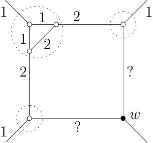 Figure 1
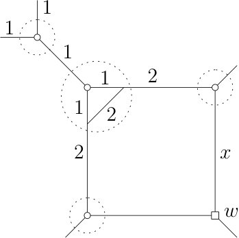 Figure 2
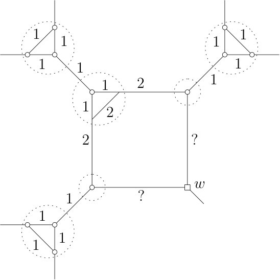 Figure 3
 Figure 4
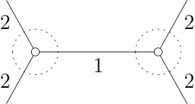 Figure 5
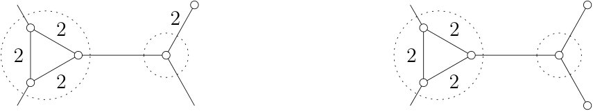 Figure 6
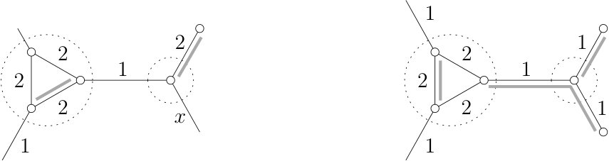 Figure 7
 Figure 8
 Figure 9
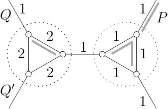 Figure 10
 Figure 11
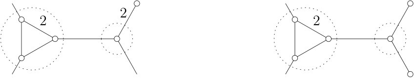 Figure 12
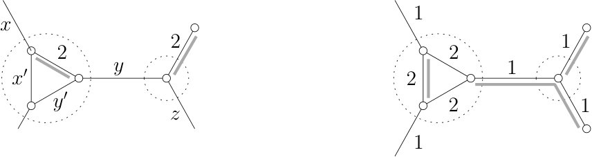 Figure 13
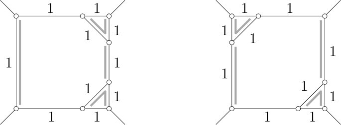 Figure 14
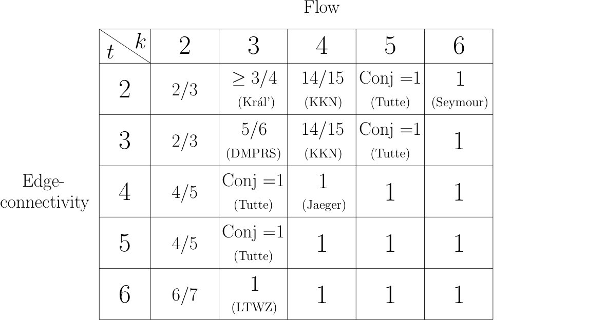 Figure 15
 Figure 16
 Figure 17
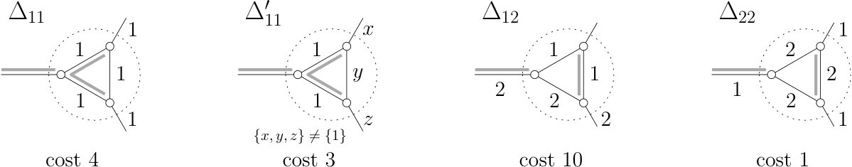 Figure 18
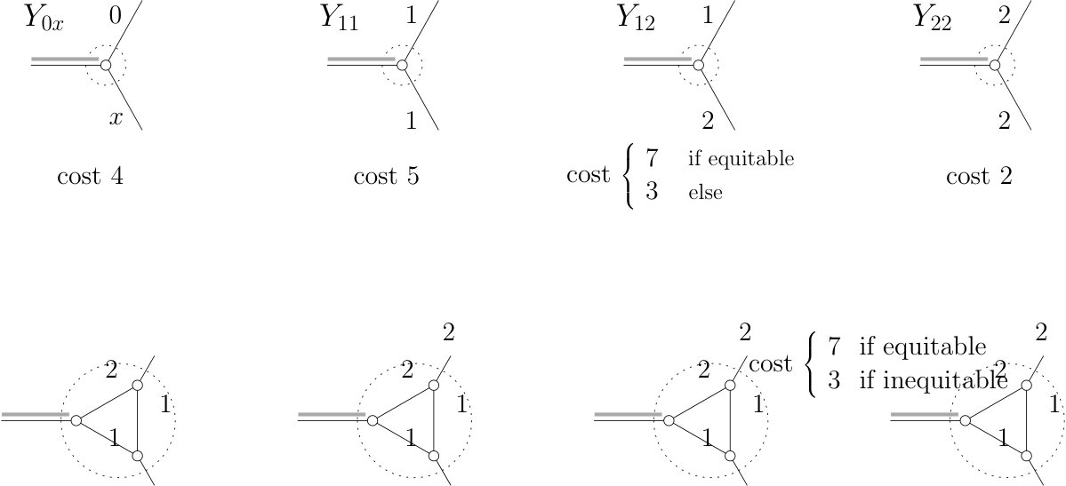 Figure 19
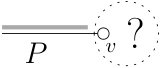 Figure 20
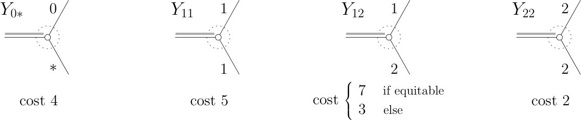 Figure 21
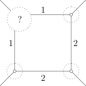 Figure 22
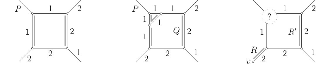 Figure 23
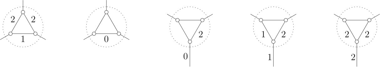 Figure 24
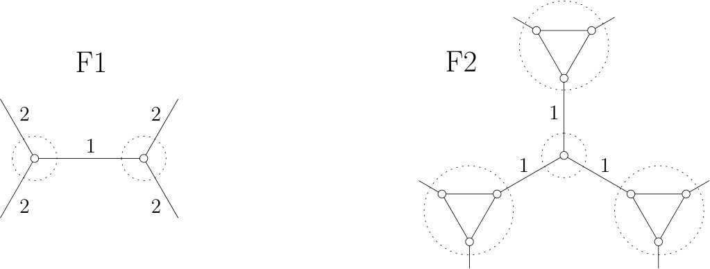 Figure 25
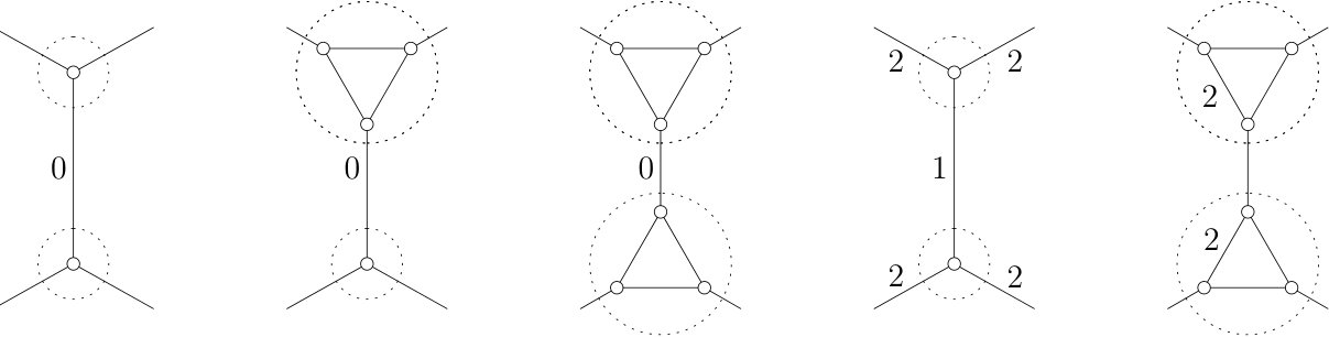 Figure 26
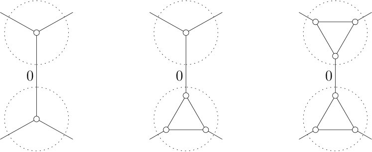 Figure 27
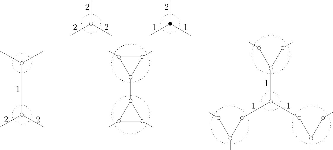 Figure 28
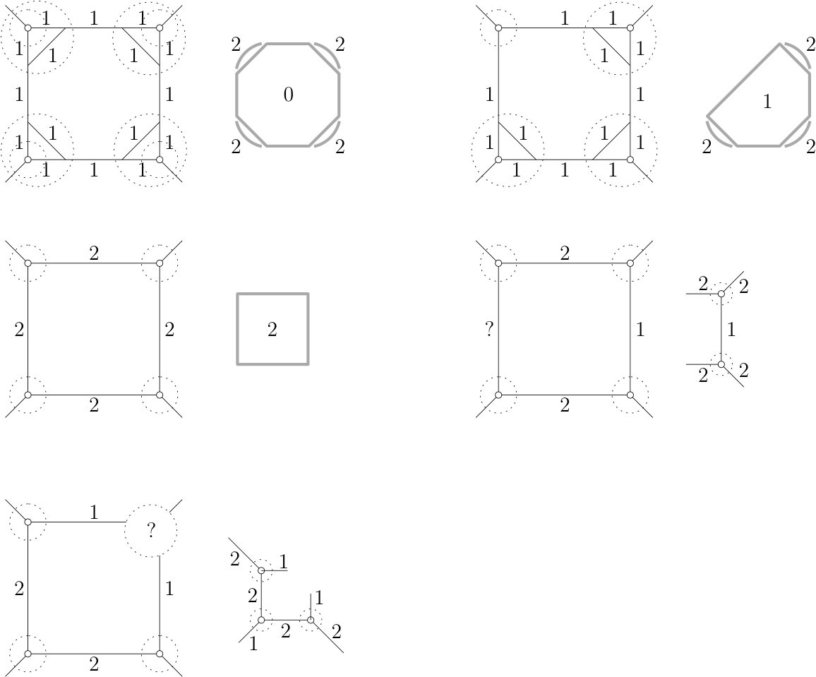 Figure 29
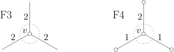 Figure 30
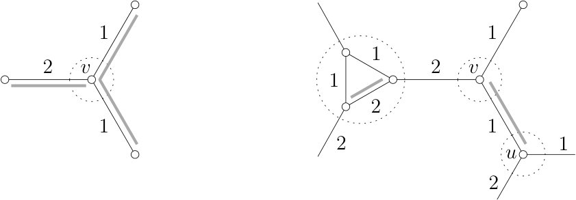 Figure 31
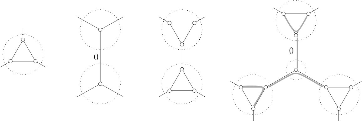 Figure 32
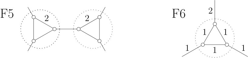 Figure 33
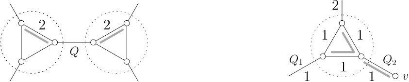 Figure 34
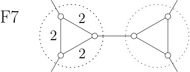 Figure 35
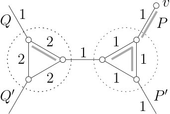 Figure 36
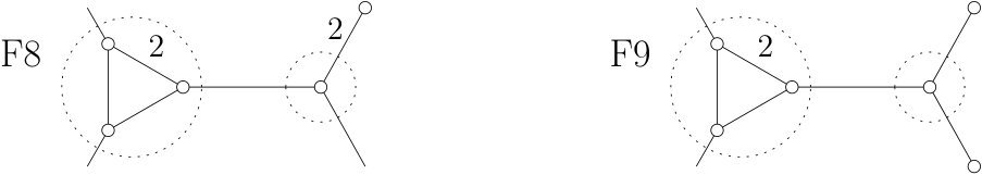 Figure 37
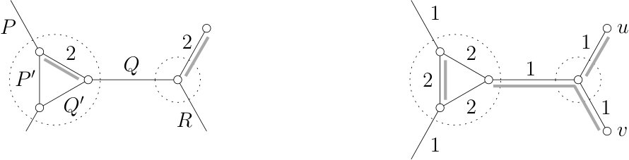 Figure 38
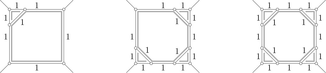 Figure 39
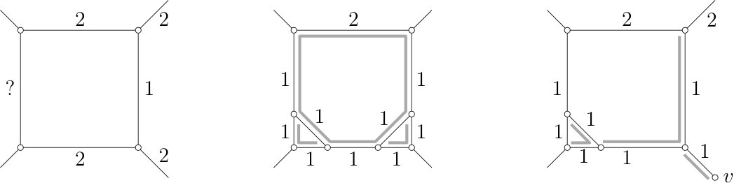 Figure 40
Peer Reviews
No public reviews on file for this paper yet. If you reviewed it on a platform where reviews are public (OpenReview, ICLR, NeurIPS, ICML), you can paste yours below so the community can read it here.
Videos
No videos yet. Explain this paper in a talk, walkthrough, or lecture? Add one.
3-Flows with Large Support
Matt DeVos Department of Mathematics, Simon Fraser University, Burnaby, B.C., Canada V5A 1S6, [email protected].
Jessica McDonald Department of Mathematics and Statistics, Auburn University, Auburn, AL, USA 36849, [email protected].
Irene Pivotto School of Mathematics and Statistics, University of Western Australia, Perth, WA, Australia 6009, [email protected].
Edita Rollová European Centre of Excellence, NTIS- New Technologies for Information Society, Faculty of Applied Sciences, University of West Bohemia, Pilsen, [email protected].
Robert Šámal Computer Science Institute of Charles University, Prague, [email protected].
Abstract
We prove that every 3-edge-connected graph has a 3-flow with the property that . The graph demonstrates that this ratio is best possible; there is an infinite family where is tight.
Contents
1 Introduction
Throughout the paper we permit graphs to have both multiple edges and loops. If is an oriented graph and is an additive abelian group, then we define a function to be a flow if it satisfies the following rule at every vertex :
[TABLE]
where () denotes the set of edges directed away from (toward) the vertex . The flow is nowhere-zero if and it is called a -flow for a positive integer if and for every . The support of is the set of all edges of with , and is denoted by . In [9] Tutte initiated the study of nowhere-zero flows by proving the following duality theorem.
Theorem 1.1** (Tutte).**
If and are dual planar graphs, then has a proper -colouring if and only if has a nowhere-zero -flow.
Based in part on this duality, Tutte ([9, 11]) made three lovely conjectures concerning the existence of nowhere-zero flows. These conjectures, known as the 5-Flow, 4-Flow, and 3-Flow conjectures have motivated a great deal of research on this subject, but despite this all three remain unsolved.
Our approach here will be to relax the notion of nowhere-zero and instead look for flows which have large support. Our main theorem is the following bound for 3-flows in 3-edge-connected graphs.
Theorem 1.2**.**
Every 3-edge-connected graph has a 3-flow satisfying
[TABLE]
Since the graph does not have a nowhere-zero 3-flow, but does (for any edge of ), the ratio in this theorem is best possible. The family of tight examples is much larger, though. Let us call tripod a graph obtained from by adding a pendant edge to every vertex. So tripod has three leaves (i.e., vertices of degree 1); identifying the leaves of a tripod produces a . Suppose is a graph obtained from a set of tripods by identifying their leaves (in any desired way). Consider any 3-flow of ; restricting such a flow to a single tripod and then contracting all edges outside the tripod produces a 3-flow of . Therefore has no flow with support larger than . An easy way to get large 3-edge-connected graphs as a union of tripods is to start with a 3-edge-connected bipartite graph such that all vertices in have degree 3. Then we truncate each vertex in , which turns it into a triangle. This triangle together with the original neighbors of form a tripod.
When we restrict our attention to planar graphs, our theorem has the following corollary (proved in the following section).
Corollary 1.3**.**
If is a simple planar graph, then there exists a function so that the number of edges with is at most .
Note that the graph also demonstrates that the above corollary gives a best possible bound. In fact, this corollary is not a new result – it is also a corollary to the Four Colour Theorem. To see this, let be a proper 4-colouring of , and assume (without loss) that the number of edges with one end of colour 3 and one of colour 4 is at most . Now the function given by is a 3-colouring with the desired properties. To our knowledge, our argument gives the first proof of this result not relying on the Four Colour Theorem.
Although the ratio in Theorem 1.2 is best possible, it seems quite possible that the same bound holds more generally for graphs which are 2-edge-connected. Unlike most results in the realm of nowhere-zero flows, our theorem on 3-edge-connected graphs does not obviously give a similar result for 2-edge-connected graphs. The best bound we have for 3-flows in 2-edge-connected graphs is the following result due to Tarsi [8] (proved in Section 2). An earlier version of this paper instead included a result by Král’ [4] with in place of .
Theorem 1.4** (Tarsi).**
Every 2-edge-connected graph has a 3-flow with
[TABLE]
More generally, we are interested in finding bounds on the maximum support of a -flow in a -edge-connected graph. For a graph and a positive integer , let be the maximum of over all possible -flows . Then, for a positive integer , we define to be the infimum of over all -edge-connected graphs. So is the best lower bound for the maximum ratio of edges covered by a -flow over all -edge-connected graphs. It is immediate that and for all . The following table indicates our present state of knowledge of for .
Tutte’s famous 5-Flow and 3-Flow Conjectures are equivalent to the assertions that and as shown in the table. Several famous theorems on flows appear here as well. For instance, Seymour’s 6-Flow Theorem [7] is equivalent to , Jaeger’s 4-Flow Theorem [1] is equivalent to , and the recent result of Lovász, Thomassen, Wu, and Zhang on 3-Flows [5] is equivalent to . The indicated result is a straightforward consequence of a variant of a theorem of Kaiser, Král’ and Norine [3] as we show in the next section. This table suggests that . This is indeed true, and will also be established in the following section by way of some standard techniques. Since is nondecreasing in both and , all values of this function are known apart from the pairs , , , , and .
In this paper we will prove that . In fact, our main theorem has a somewhat stronger “choosability” form related to group-connectivity as introduced by Jaeger, Linial, Payan, and Tarsi [2]. Instead of insisting that the function is a flow, we may instead ask for the sum involved at the vertex , (i.e., ) to take on certain prescribed values at each vertex . Let us return to a general setting to put these definitions in place. Assume that is an oriented graph, let be an abelian group (written additively) and let . The boundary of is the function given by the following rule for every :
[TABLE]
We recall that and denote the set of edges directed away from and toward respectively. If we think of as indicating a circulation of fluid, then tells us how much is leaving the network at . Note that by definition, the function is a flow if is identically zero. If we sum the boundary function over all vertices, then whatever value is assigned to an edge will get added once and subtracted once, so it has no effect. This gives the following useful identity
[TABLE]
which holds for every function . In general, we say that a function is zero-sum if . The general form of our main theorem may now be stated as follows.
Theorem 1.5**.**
If is an oriented 3-edge-connected graph and is zero-sum, then there exists so that
, and 2. 2.
**
To see that this theorem implies Theorem 1.2, simply apply it with to choose a flow with . Now using Tutte’s equivalence between nowhere-zero modular and integer flows [10] (applied on the support of ) we deduce that has a 3-flow with support of size at least as desired.
Unlike our earlier theorem, in the case of Theorem 1.5 the assumption of 3-edge-connectivity is necessary. To see this, take an arbitrary oriented 3-edge-connected graph with and modify it by subdividing every edge twice (thus forming a directed path of three edges). Now define by the following rule:
[TABLE]
For every 3-edge path with both interior vertices of degree 2, a straightforward check reveals that every function which satisfies will have the property that assigns all three edges of distinct values. Therefore, every such function will satisfy . Consequently, Theorem 1.4 does not extend from -flows to -connectivity.
2 Flow and Colouring Bounds
In this section we will prove Corollary 1.3 and some of the results stated in the table of Figure 1. As in the proof of Theorem 1.5, we may use Tutte’s theorem to work with flows in any abelian group of order , instead of with integer -flows. We will do this implicitly throughout this section.
Proof of Corollary 1.3:.
Let be a simple planar graph and let be the dual of . Since is simple, is 3-edge-connected. By Theorem 1.2 we may choose a flow with . Let be the graph obtained from by contracting the edges with -value zero. Now the restriction of to is a nowhere-zero 3-flow. It follows by Theorem 1.1 that the dual of has a proper 3-coloring. Since is obtained from by deleting the edges corresponding to , the result holds. ∎
Proof of Theorem 1.4:.
By Seymour’s 6-flow theorem we may choose a nowhere-zero flow of . Over all such possible choices for , we claim that a fixed edge receives each of the five flow values equally often. To see this, recall that the number of nowhere zero -flows in can be calculated via a contraction-deletion formula, by successively choosing edges until all that remains are loops and bridges. The same procedure can be used to count the number of nowhere zero -flows with the property that receives a fixed flow value of . The process of contraction and deletion does not depend on this value . Moreover, the number of nowhere-zero flows (where has flow value ) in each of these terminal graphs is independent of . So, we indeed get our claim. In particular, each edge receives the value 3 in exactly one fifth of the possible choices for . This means that on average one fifth of the edges in receive 3, and we may choose a particular so that no more than one fifth of the edges in receive 3. Define by reducing each flow value in modulo 3. Note that is indeed a flow on , and its only zero edges correspond to edges receiving 3 under . ∎
Before we get to prove our result on approximative 4-flows, we need a version of a theorem of Kaiser, Král’ and Norine [3].
Theorem 2.1** (Kaiser, Král’, Norine [3]).**
Let be a 2-edge-connected cubic graph and a weighting function on the edges. Then contains two perfect matchings , such that .
Proof.
We follow closely the proof of Theorem 1 in [3]. We also refer the reader there for more background on the perfect matching polytope theorem. First, we define for every edge of and observe that is in the perfect matching polytope (here we use the fact that has no bridge). That means that is a convex combination of for some perfect matchings , , …, . It follows that we can find such that . (We use to denote the scalar product of with and for the characteristic function of .)
Still following [3], we choose if and otherwise. We show now, that is also in the perfect matching polytope: We need to verify that for every odd edge cut . If , this is obviously true. As is bridgeless, we only need to consider the case . We recall how was chosen. It is one of the perfect matchings that have as their convex combination. As (by definition) and for every (as is a perfect matching and is an odd cut), it follows that for every . Therefore, .
We define . As is a convex combination of characteristic functions of perfect matchings, there is a perfect matching , such that , as claimed. ∎
Next we prove another theorem claimed in our introduction. For a graph and a pair of edges which are both incident with the vertex , we lift and by creating a new vertex and changing to have as an endpoint instead of .
Theorem 2.2**.**
Every 2-edge-connected graph has a 4-flow with .
Proof.
We may assume that is not Eulerian, since in this case it has a 2-flow with support . It follows from Mader’s Splitting Theorem [6] that we may repeatedly perform the aforementioned lift operation to obtain a graph which is subcubic and still cyclically 3-edge-connected. Let be the graph obtained from by suppressing every vertex of degree 2. Then each edge corresponds to a path of and we let be the length of this path.
It follows from Theorem 2.1, that there exists a pair of perfect matchings in so that . For define the function by the rule that if the edge of associated with is in and otherwise . Now is a -flow of with support of size as desired. ∎
Note that the bound in Theorem 2.2 is achieved by the Petersen graph.
Theorem 2.3**.**
For every , .
Proof.
For every there exists a -regular graph which is -edge-connected. If is a 2-flow of , then for every vertex at least one of the edges incident with will not be contained in . It follows that thus giving the bound .
For the other direction, let be an arbitrary -edge-connected graph. We may assume that is not Eulerian, since in this case has a 2-flow with support . As in the previous proof, we repeatedly apply Mader’s Splitting Theorem to vertices with even degree and to vertices with odd degree , and we let be the resulting graph. Let be the graph obtained from by suppressing vertices of degree 2; so every corresponds to a path of and we let be the length of this path.
It follows from Edmond’s Matching Polytope theorem that there exists a list of perfect matchings in so that every edge of is contained in exactly of these matchings. So, we may choose so that . Now in the original graph there is a 2-flow with support and thus . ∎
3 Ears
Although Theorem 1.5, which we wish to prove, concerns 3-edge-connected graphs, our proof will involve a reductive process which encounters graphs which are only 2-edge-connected. In preparation for this, we will establish some terminology and tools for working with 2-edge-connected graphs.
3.1 Ear Decomposition
A well-known basic result in graph theory is the ear decomposition theorem which asserts that every 2-connected graph has a certain recursive structure. For our purposes we will want to work with edge-connectivity, and it will be helpful to recast this basic concept in this alternate setting. Since this notion is extremely close to the original, we will adopt the same terminology. Accordingly, we now define an ear of a graph to be a subgraph which satisfies one of the following:
- •
is a nontrivial path (i.e., a path with at least two vertices), all interior vertices of have degree in , but both endpoints have degree at least in .
- •
is a cycle of containing exactly one vertex with degree in .
- •
is a cycle.
For an arbitrary graph we let denote the graph obtained from by deleting all isolated vertices (i.e., vertices of degree 0). If is an ear of , then removing brings us to the new graph . We define a partial ear decomposition of a graph to be a list of subgraphs of satisfying the following:
whenever . 2. 2.
is an ear of the graph obtained from by removing .
A partial ear decomposition is called a full ear decomposition if . Note that in this case the first graph must be a cycle. If is a full ear decomposition of , then a straightforward induction implies that each of the graphs will be 2-edge-connected, so in particular, any graph with a full ear-decomposition must be 2-edge-connected. Conversely, for any 2-edge-connected graph we may construct a full ear-decomposition greedily starting from an arbitrary cycle (if we have chosen and there is an edge , then by Menger’s Theorem there are two edge-disjoint paths starting at the ends of and ending in and the union of these paths together with contains a suitable choice for ). This yields the following basic property.
Proposition 3.1**.**
A graph is 2-edge-connected if and only if it has a full ear decomposition.
3.2 Weighted Graphs and Ear Labellings
We define a weighted graph to be a graph equipped with a function , and we call a zero-sum weighted graph if is zero-sum. In preparation for the proof of Theorem 1.5, we now introduce a framework to move from one weighted graph to another by removing ears.
For our main theorem we consider an oriented zero-sum weighted graph and we are interested in finding a function with boundary and large support. Let us take a moment to consider the possible behaviours of such a function on an ear. So, let be an ear of and express as either a path or closed path with vertex-edge sequence so that have degree 2 in (i.e., if is a cycle containing a vertex of with degree , then this vertex is ). Assume further (for simplicity) that every edge is oriented from to . If we have chosen the value and we wish for our function to satisfy , then (assuming ) we must assign . This in turn forces the value of and all the remaining edges of (in general, ). So, when constructing our function we have just a single degree of freedom for each ear. These choices will be significant for us, so we will introduce a little terminology to work with them. If is an ear of , a function is called an ear labelling if for every vertex which is in the interior of the path . The following observation is a straightforward consequence of this discussion (together with the basic fact that when is a cycle, every function for which and agree on all but one vertex will satisfy , since these two functions are both zero-sum).
Observation 3.2**.**
Let be an ear of the oriented zero-sum weighted graph . Then there are exactly three distinct ear labellings of , and every has value 0 in exactly one of these labellings. In fact, in the above-defined orientation we may assume (indices modulo 3).
Since we are looking to construct functions which have large support, we will naturally be interested in ears of which have an ear labelling with large support. If are the ear labellings of , then by the above discussion, the average size of the support of an ear labelling will be precisely . When is a multiple of 3, we may have for . (Equivalently, still assuming the “forward orientation” of , we may have .) In this extreme case we say that is equitable, and in all other cases we call inequitable. When is not a multiple of 3 (or more generally when is inequitable), there exists at least one ear labelling with and our proof will frequently exploit this. Indeed, the key to our argument is getting a small advantage for each inequitable ear.
In preparation for this we now introduce a general definition. If is a subgraph of and , we define the gain of to be
[TABLE]
The following lemma gives our basic tool for finding good ear labellings. We will use this extensively in the remainder of the paper.
Lemma 3.3**.**
Let be a weighted graph. If is an inequitable ear of such that where , then has an ear labelling with . If is equitable, then it has an ear labelling with .
Proof.
Choose an ear labelling of for which is maximum, and note that our assumptions imply that , i.e., . This gives as desired. ∎
Next we introduce some terminology to facilitate the process of deciding on a particular ear labelling, and then removing this ear from the weighted graph. If is an ear of and is an ear-labelling, we define the -removal of (from ) to be the weighted graph equipped with the weight function given by the following rule (we set if )
[TABLE]
Since and both sum to zero, the same holds for the function . It follows that the function will be zero-sum. The following straightforward observation shows that we can combine a function with boundary with our ear labelling to obtain a function on with boundary .
Observation 3.4**.**
Let be an oriented zero-sum weighted graph, let be an ear, let be an ear labelling of , and let be the -removal of . If satisfies , then the following function has :
[TABLE]
4 Setup
In this section we will state our workhorse lemma, and use it to prove our main theorem. Then we will set the stage for our proof of this lemma by fixing a minimal counterexample to it, and establishing some initial properties of this weighted graph.
4.1 Framework
Before we are ready to state our main lemma (Lemma 4.1 below), let us pause to introduce the type of connectivity we will be working with. Throughout the heart of the proof of the central lemma we will work with graphs which are subdivisions of 3-edge-connected graphs. Since we are permitting loops, and any 1-vertex graph is 3-edge-connected, it is possible for to be a cycle or more generally a collection of cycles which intersect at a common vertex. So, is a subdivision of a 3-edge-connected graph if and only if is a 2-edge-connected graph which is cyclically 3-edge-connected (i.e., if is an edge-cut which separates cycles, then ).
As seen in the previous section, ears with different lengths modulo 3 will behave differently when constructing our desired function. To deal with this behaviour we will introduce a bonus function which assigns to each ear a value which indicates in some sense the amount we expect to gain from it. For an ear we define the bonus of as follows:
[TABLE]
For a subgraph which is a union of disjoint ears, that is (where each is an ear in ) we define . (We warn the reader of a possible confusion: the ’s do not necessary form an ear decomposition of , and they may also not be ears in , but only ears in .) So is the sum of the bonuses of all of the ears of . With this terminology in place, we are finally ready to state the workhorse lemma which will imply Theorem 1.5.
Lemma 4.1**.**
Let be an oriented zero-sum weighted graph and assume that is a subdivision of a 3-edge-connected graph. Then there exists satisfying:
- •
,
- •
.
Now let us see that this lemma implies our main theorem.
Proof of Theorem 1.5:.
Let be a 3-edge-connected graph and let be zero-sum. Every edge of is an ear with length 1 mod 3. So, the lemma gives us a function with and , as desired. ∎
We try now to preview the main ideas of the proof, before we get into the lengthy details. It was crucial to find the proper setting: we have generalized Theorem 1.2 to Theorem 1.5 (about flows with a given boundary). Then we have extended it even further by defining an appropriate bonus system: Lemma 4.1 provides a result about a richer class of graphs. Building upon this choice of graphs, we will be able to find many types of reductions to a smaller graph, while staying in the class. These reductions involve deleting edges or vertices of a graph (Lemma 4.15 and 4.16) or even pairs of adjacent vertices (Observation 7.9).
4.2 Minimal Counterexample
Assume (for a contradiction) that Lemma 4.1 is false, and choose a counterexample for which is minimum. We will spend the rest of the paper discussing properties of , building towards a contradiction. We start with two very straightforward lemmas concerning . The first one shows that is not too basic in structure, the second one shows it has no equitable ear.
Lemma 4.2**.**
* has at least two vertices with degree at least .*
Proof.
Suppose (for a contradiction) that has at most one vertex of degree at least . Apply Lemma 3.3 to choose an ear labelling with for every ear of . Let be the union of these functions and note that . It follows from our construction that holds at every vertex with . Since and are both zero-sum, we conclude that , which is a contradiction. Hence has at least two vertices with degree at least . ∎
If is a weighted graph and , then contracting gives a new weighted graph where the underlying graph is obtained from by contracting the edge to form a new vertex , and the weight function is given by the following rule:
[TABLE]
Note that if is zero-sum, then will also be zero-sum.
Lemma 4.3**.**
If is an ear of with ear labellings , then there do not exist so that for . In particular, has no equitable ear.
Proof.
Suppose to the contrary that there exist such edges . Let be the weighted graph obtained from by contracting , let be obtained from by contracting , and let be obtained from by contracting . Now is either empty (in which case was equitable and had bonus 0) or it induces an ear of with the same length modulo 3 as . It follows from our definitions that , so by the minimality of our counterexample, we may choose a function with and . Now we will step back from to by reversing the contraction of . Since any two zero-sum functions which agree on all but one vertex also agree on the last, we may extend by choosing a value for in such a way that . Repeating this argument to reverse the contraction of and then results in a function with . The restriction of to is an ear labelling, so by our assumption for exactly one . This function satisfies the conclusion of Lemma 4.1, thus giving us a contradiction. Therefore no such ear may exist. In particular this implies that has no equitable ear. ∎
4.3 Contraction
In order to handle more general situations, we will now establish some tools for finding subgraphs of which we can contract. In many of our arguments, we will be interested in removing a sequence of ears which have nonzero length modulo 3, and we will call on Lemma 3.3 to find suitable ear labellings. In light of this, it is natural (and helpful) to introduce a concept of gain for a partial ear decomposition. Let be a graph, let be a partial ear decomposition of , and assume that where for every . Then we define (motivated by Lemma 3.3) the gain of to be . The following easy lemma gives a first use of this concept, explaining the connection to the gain of an ear labelling.
Lemma 4.4**.**
Let be an oriented zero-sum weighted graph with a full ear decomposition . Then there exists with so that is at least the gain of .
Proof.
Starting with and working down to we apply Lemma 3.3 to choose an ear labelling of and then replace by the -removal of . If is the union of these functions, then by repeated applications of Lemma 3.4, we have and by construction we have that is at least the gain of . ∎
Next we define a notion of contractible based on this concept of gain.
Definition 4.5**.**
Let be a union of ears. We say that is contractible if there exists a full ear decomposition of with gain at least .
For clarity, we note that , where , …, are the ears of that comprise . However, the ’s and the ’s are, in general, different (each of the ’s is a union of some of the ’s).
Also note that, in particular, a contractible subgraph is 2-edge-connected. The next lemma shows that this definition captures the desired notion.
Lemma 4.6**.**
* has no contractible subgraph.*
Proof.
Suppose (for a contradiction) that is a contractible subgraph of and that is the indicated ear decomposition of . Note that must be connected since it has a full ear decomposition. Let be the weighted graph obtained from by contracting all of the edges in . By the minimality of our counterexample we may choose a function with and . Extend to have domain by setting for every . Now and agree on every vertex in . We define by the rule . Since and are both zero-sum, the function will also be zero-sum. Using Lemma 4.4 we may choose a function with and . Now the union of and has boundary and gain at least , which is a contradiction. ∎
Next we call on the concept of contractible to eliminate some additional subgraphs of .
Lemma 4.7**.**
There does not exist a cycle satisfying one of
* is the union of at most two ears and ,* 2. 2.
* is the union of three or four ears and .*
Proof.
In the former case, and has a full ear decomposition (consisting of the entire cycle ) of gain , so is contractible. In the latter case, and has a full ear decomposition of gain , so it is contractible. ∎
4.4 Deletion
Next we will introduce some tools to facilitate deletion arguments. Unlike contraction which automatically preserves our desired edge-connectivity, we will need to be careful when deleting.
Definition 4.8**.**
A subgraph is reducible if there exists a partial ear decomposition of together with functions for satisfying the following properties:
- •
,
- •
* is empty or is a subdivision of a 3-edge-connected graph, *
- •
The function is an ear labelling of in the -removal of from from the -removal of from .
- •
The weighted graph that is the -removal of from from the -removal of from satisfies .
The following observation shows that our minimal counterexample cannot contain a subgraph of this type.
Observation 4.9**.**
* does not have a reducible subgraph .*
Proof.
Suppose (for a contradiction) that such a subgraph exists and let and and be as in the above definition. By the minimality of the counterexample (and by the second property in the definition of reducible) we may choose a function with and . Now repeatedly applying Observation 3.4 to gives us a function with and which is a contradiction. ∎
We will apply the above observation repeatedly, but we will begin with an easy instance.
Lemma 4.10**.**
* does not have either of the following:*
- •
a cycle which is an ear,
- •
a cycle consisting of two ears containing a vertex of degree 3 in .
Proof.
If has a cycle which is an ear, then Lemma 4.2 (and the assumption that is a subdivision of a 3-edge-connected graph) implies that must contain a vertex of degree at least in . Thus, removing does not merge two ears of into one, implying . Lemma 3.3 allows us to choose an ear labelling of with and it then follows that is a reducible subgraph (contradicting Observation 4.9).
Next suppose that has a cycle consisting of two ears so that an endpoint of and has . Let be the other endpoint of these two ears, and let be the third ear incident to . By Lemma 4.7 we have , so we may assume (without loss) that . Therefore, by Lemma 3.3 (and Lemma 4.3) we may choose an ear labelling of with gain at least 16. If is the -removal of , then we have that is a subdivision of a 3-edge-connected graph, as the ears and merge in . If has degree at least 4 in , then there are just three ears of which are not ears of . If has degree 3 in , then since is a subdivision of a 3-edge-connected graph, must be incident to , and must consist of only these three ears. Hence, in either case, . Thus is reducible, giving us a contradiction. ∎
4.5 Pushing a 3-Edge Cut
We have introduced the concept of a reducible subgraph and this will be key in our proof. However, in order for a subgraph to be reducible, it must be the case that is a subdivision of a 3-edge-connected graph (or it is empty). So, in our search for reducible subgraphs, we will need to have some tools for finding subgraphs which we can delete so as to maintain our connectivity. This section gives the first of these tools. It is based on a simple minimality property for 3-edge-cuts. Once we have this in place, we will apply it to construct a new graph which will be convenient for our operations.
For any subset of vertices of a graph, we let denote the number of edges with exactly one endpoint in . The proof of our main tool from this section is based on uncrossing arguments that call on the following inequalities which hold for any two subsets of vertices.
[TABLE]
Lemma 4.11**.**
Let be a 3-edge-connected graph and let be minimal subject to the following conditions
, 2. 2.
* induces a graph containing at least two cycles.*
If has both ends in , then every 3-edge-cut of containing has the form where induces a graph containing at most one cycle.
Proof.
Suppose that is a 3-edge-cut of with , and consider the Venn diagram on given by the sets and as depicted in the figure below. By possibly swapping with its complement, we may assume that is nonempty. First suppose that . Then inequality (1) gives us , but then the 3-edge-connectivity of implies . It now follows from the minimality of that is a subset of which induces a graph containing at most one cycle, as desired.
Thus, we may assume that all four sets in our Venn Diagram are nonempty. Now the inequalities (1) and (2) imply that , but this is impossible. (For instance , so our present conditions violate parity.) ∎
In order to productively use this lemma, we will need to show that our graph is not one of a couple of small graphs. One of these graphs is a two vertex graph with exactly three edges none of which is a loop, which we call Theta.
Lemma 4.12**.**
* is not isomorphic to a subdivision of either or Theta.*
Proof.
By Lemma 4.10, is not a subdivision of Theta. Now suppose (for a contradiction) that is isomorphic to a subdivision of . If there is an ear of with length 0 mod 3, then it has an ear labelling with gain at least 24 (by Lemma 3.3 and 4.3), and thus is a reducible subgraph since . If has an ear with length 2 mod 3, then setting to be the unique ear of which does not have an end in common with , we may construct a full ear decomposition using and which has gain at least (again, Lemma 4.4 shows that is not a counterexample). So, we may assume that every ear of has length 1 mod 3. Again in this case we find a full ear decomposition of with gain at least 24, thus giving us a contradiction. ∎
We need just one more simple property of before we can take advantage of Lemma 4.11.
Lemma 4.13**.**
* has a 3-edge-cut so that induces a subgraph containing at least two cycles.*
Proof.
First suppose that does not have an edge-cut of size 3. In this case, Lemma 3.3 implies that every ear is a reducible subgraph, so is not a minimal counterexample. Therefore, we may assume that has some edge cut with . If neither nor satisfy the lemma, then each of these sets induces a graph with at most one cycle. If induces a graph with no cycles, then since is a subdivision of a 3-edge-connected graph and , is a subdivision of . If induces a graph with a unique cycle , then Lemma 4.10 says that is not an ear nor it is composed of two ears with a vertex of degree three. So must be the union of exactly three ears whose endpoints all have degree 3 in (otherwise more than three edges are incident to , so would have a second cycle or a small edge-cut). A similar argument for shows that must be a subdivision of either Theta, or the graph Prism depicted below. The former two cases are impossible by the previous lemma; in the last case choosing to be the complement of a vertex of degree 3 yields a suitable edge-cut. ∎
4.6 Creating
With the above lemma in place we shall now choose a set so that and the graph induced by contains at least two cycles, and subject to this we choose minimal. Let be the ears of containing an edge of and define to be the set of all vertices which are not in and are not interior vertices in , , or . We define to be the weighted graph obtained from by identifying to a single new vertex , and deleting any loop at . (As a typographical reminder, when depicting the vertex in our figures we will use a ). The following observation is an immediate consequence of this definition and Lemma 4.11.
Observation 4.14**.**
If is a 3-edge-cut of with , then one of the following holds:
, 2. 2.
The graph induced by contains at most one cycle.
Note that every ear of is also an ear of . The three ears of which are incident with the vertex will be called unusable since we have little control over the 3-edge-cuts of which meet these three ears. Every other ear of will be called usable. We say that a cycle with is an inner triangle if . Note that in this case, Observation 4.14 implies that has no chords. By Lemma 4.10, is a union of three distinct ears. Hence it contains exactly three vertices of degree 3, while all other vertices of have degree 2 (hence the name triangle). Since is a subdivision of a 3-edge-connected graph, any two distinct inner triangles must be vertex disjoint. We say that an ear of is inner if it is contained in an inner triangle and it is outer otherwise. The following lemma follows from Lemma 4.11 applied to the graph obtained from by suppressing the degree 2 vertices.
Lemma 4.15**.**
Let be a usable ear of and let .
If is inner, is a subdivision of a 3-edge-connected graph. 2. 2.
If is outer, then the only 2-edge-cuts of separating cycles have the form where contains a unique cycle which is an inner triangle in (and contains an end of ).
So, in short, removing an inner ear always results in a graph which is a subdivision of a 3-edge-connected graph, while removing an outer ear may result in a graph with one or two cyclic 2-edge-cuts. If one of these cuts is of the form for some cycle with and , then induces a graph with exactly one cycle . Thus deleting any ear in and then deleting one of the two ears in in the resulting graph produces a subdivision of Theta, which is a subdivision of a 3-edge-connected graph. All other cyclic edge cuts produced by deleting an outer ear appear as where contains a unique cycle which is an inner triangle (there are at most two such cycles , one at each end of the removed outer ear ). We may further modify by removing an ear of contained in so as to return to a graph which is a subdivision of a 3-edge-connected graph. This basic reduction technique will be exploited at great length throughout our proof.
A similar technique is based on the following lemma: we can remove three ears adjacent to the same vertex/inner triangle, and then we remove up to three more ears, one from each inner triangle that now forms a 2-edge-cut. Again, this procedure yields a subdivision of a 3-edge-connected graph.
Lemma 4.16**.**
Let , , be usable ears of such that
either all of , , and are adjacent to the same vertex of degree 3, 2. 2.
or all of , , and are adjacent to the same inner triangle .
Consider the graph (in the first variant) or (in the second variant). Then the only 2-edge-cuts of separating cycles have the form where contains a unique cycle , which is an inner triangle in (distinct from ) and contains an end of some (, , or ).
Proof.
By arguments similar to those for Lemma 4.15, it is easy to see that deleting exactly one of and , say , and possible modification of its incident triangles yields a subdivision of a 3-edge-connected graph. Now in the vertex case or in the triangle case (where is the leftover of after modification of ) forms a new ear. Delete the ear and possibly modify its incident triangles. Again, by arguments similar to those for Lemma 4.15, the resulting graph remains a subdivision of a 3-edge-connected graph. ∎
Going forward, we will ignore the original graph and instead focus our attention on when searching for contractible or reducible subgraphs. However, any contractible subgraph of which contains only usable ears will also be a contractible subgraph of . Similarly, if is a reducible subgraph of which contains only usable ears, then will also be a reducible subgraph of since the graph will also be a subdivision of a 3-edge-connected graph. So in short, as long as we avoid the unusable ears, we are free to operate in .
5 Forbidden Configurations
In this section we will establish a number of results which give us information about our minimal counterexample . In order to facilitate calculations, we will introduce some graphical notation for working with possible subgraphs of . When depicting a subgraph of we will use an open circle to indicate a vertex with degree which is not , and we will use a to denote the vertex (a vertex which might or might not be receives no symbol). If there is an ear with ends , then this will appear as a line segment between and and we will sometimes mark this segment with a 0, 1, or 2 to indicate the length of mod 3 (we will not indicate vertices of degree 2). Finally, we will draw a dotted circle around an inner triangle and will draw a small dotted circle around a vertex to indicate that it is not in an inner triangle (such vertex will be called a triad). We call these drawings configurations, and we will say that a configuration is forbidden if the corresponding subgraph cannot appear in .
Lemma 5.1**.**
Every inner triangle in appears in a configuration of one of the following three types:
**
Furthermore, if is an ear with length 2 mod 3 which is contained in an inner triangle, then for every ear labelling of with gain at least 16, both newly formed ears of the -removal of are equitable.
Proof.
Consider the configurations appearing in the figure below.
In the rightmost configuration, the thick gray lines indicate a contractible subgraph by Lemma 4.7, so this configuration is forbidden. For the two configurations on the left in the figure, the thick gray lines indicate a partial ear decomposition consisting of just a single ear which we call .
If has length 0 mod 3 (as on the left), then since is not equitable (Lemma 4.3), we may choose an ear labelling with gain at least 24 by Lemma 3.3. The -removal of is a weighted graph which is still a subdivision of a 3-edge-connected graph. Since there are just 5 ears of which are not ears of , we have and we conclude that is reducible. Thus, every inner ear of has nonzero length mod 3.
Next suppose that is an inner ear with length 2 mod 3 as in the middle and let be the ears as shown in the figure. By Lemma 3.3 we may choose an ear labelling of with and we let denote the -removal of . Now is an ear of , and if this ear is not equitable, then and we have a reducible subgraph. Therefore, must be equitable in . Since cannot have length 0 mod 3 it must be that one of has length 1 mod 3 and the other has length 2 mod 3.
Combining the above arguments we deduce that every inner triangle must have one of these three types, as desired. ∎
Lemma 5.2**.**
No usable ear has length 0 mod 3.
Proof.
Consider the configurations appearing in the figure below.
For each of these configurations the figure indicates a partial ear decomposition. Let be the outer ear with length 0 mod 3 as indicated and note that since is not equitable (by Lemma 4.3), we may choose an ear labelling of with gain at least 24 (Lemma 3.3). As usual, we will consider the -removal graph . If neither end of is in an inner triangle, then is cyclically 3-edge-connected, so is reducible (clearly, ). Next suppose that some endpoint of , call it , is contained in an inner triangle. Then by Lemma 5.1, both of the ears of the inner triangle ending at , call them and , must have length 1 modulo 3. In the graph it follows that will be an ear with length modulo 3, so we may choose an ear labelling with gain at least 16. Now after forming the -removal we have repaired the connectivity problem caused by this inner triangle when we removed . Doing the same if necessary at the other end of (if it is also contained in an inner triangle) gives us a reducible subgraph. ∎
Our past two lemmas are rather easy reductions, but already give considerable structure to the graph . These two lemmas already exhibit most of the basic ideas in our process, but we will need to consider rather more complicated configurations in going forward.
5.1 Endpoint Patterns
In the proof of our last lemma, after removing a certain outer ear, we needed to remove a little more to fix cyclic 2-edge-cuts caused by inner triangles. In this section we will introduce some terminology to assist in doing the accounting in such circumstances. So our setup for this section is as follows: is an outer ear that we have decided to remove as shown in the figure below.
We will focus our attention on just one end of which we call . If has degree at least four, then removing will not cause any ears at this end to merge. If is a triad or in a cycle with , then there are two other ears, say incident with and removing will cause and to merge into a single ear. In this case we will say that has endpoint pattern , , , or at depending on which of the configurations in the following figure it corresponds to. Each of these patterns is associated with a cost which indicates the difference between the bonuses of and in the original graph and the bonus of the ear in the new graph obtained by removing (so this does not take into account the cost or gain from removing ). Note that if has one of these endpoint patterns, then we don’t need to worry about connectivity at this end after the removal of .
So, for instance has a cost of 5 since we have two ears of bonus 4 which merge to form an ear of bonus 3 in the new graph. There is one special pattern here, which has a variable cost depending on whether the newly formed ear (which will have length 0 mod 3) is equitable or not.
Next we consider the situation where we wish to remove an ear and we are interested in what happens at some end of , but this vertex is contained in an inner triangle . In this case, when we remove to form the graph , this new graph will have a 2-edge-cut separating from the rest of the graph. So, in order to maintain our desired connectivity, we will need to remove one of the two ears which comprise in the graph . It will be convenient to absorb all of this in our notion of cost. So, below we introduce four endpoint patterns , , , and with associated costs. (The subscripts and in indicate that the two ears of the inner triangle which have as an end have lengths and modulo 3.) In each case the cost gives an upper bound on the drop in bonus at this end minus the gain of the additional ear which is removed (when computing this drop in bonus, we count the five ears other than which have an end in the inner triangle).
So, for instance, the cost of is because in moving from to we lose a bonus of 4 for all 5 of the edges marked 1 for a total of , we get a bonus of 0 or 4 in for the newly formed ear since it has length 0 mod 3 (and might be equitable), and we get for the gain of the ear which is removed. In endpoint pattern , if either or the new ear obtained by deleting the two marked ears in the inner triangle is inequitable, then the cost is ; otherwise and and the total cost is 3. Note that the endpoint pattern cannot appear as the endpoint pattern of an ear with length 1 modulo 3 and similarly cannot appear on an ear with length 2 modulo 3. Next we will use this framework to establish some forbidden configurations.
5.2 Forbidden Configurations
Lemma 5.3**.**
The following configurations are forbidden.
**
Proof.
First consider the configuration on the left, and let be the ear marked as having length 1 mod 3 in this figure and assume its ends are . The partial ear decomposition given by has gain 8, and the bonus of is 4. Since the endpoint patterns associated with removing at and are both of cost 2, this gives a reducible subgraph. Although it is obvious in this case, let us note that this endpoint cost calculation would not be valid if in the graph obtained by removing , both and were contained in a single ear. In general we will need to be careful to ensure that these endpoint cost calculations are independent.
Next consider the configuration on the right, let be the ears marked as having length 1 mod 3 in this figure, and let be the common endpoint of . Now is a partial ear decomposition with gain 24 and the bonus of is 12. Since the endpoint costs associated with removing each (at the endpoint other than ) are all at most 4, this gives a reducible configuration. Again, there is a potential danger here that there is an outer ear with an end in two of the inner triangles from this configuration (as this would invalidate our cost calculation), but this would result in a 3-edge-cut of of a type that contradicts Observation 4.14, so it does not happen. Also note that the removal of is possible according to Lemma 4.16. ∎
In preparation for our next forbidden configurations, we will prove a couple of lemmas which will help us to control ears of length 1 mod 3 and allow us to arrange for the cost of endpoint pattern to be 3 (instead of 7) in certain cases.
Lemma 5.4**.**
If is a usable ear of with length 1 mod 3, then .
Proof.
Suppose (for a contradiction) that has length 1 mod 3 and . By Lemma 4.3 there is an ear labelling of with . So . If is an inner ear then it is a reducible subgraph. Otherwise, is an outer ear with bonus 4, and the endpoint patterns at the ends of each have cost at most 7, so may be extended to a reducible subgraph. ∎
Lemma 5.5**.**
Let be a weighted 2-edge-connected graph, let have and assume that are distinct ears of with endpoint . If and is not equitable, then there exists an ear labelling of with gain 8 so that in the -removal of , the ear is not equitable.
Proof.
Let be the ear labellings of , and suppose that is the zero function (so have support ). Let the ear labellings of () be denoted () for . When we perform a -removal of , the resulting weighted graph will have as an ear, and each ear labelling of this ear will have the form for some . It follows from basic principles that (working with our indices modulo 3) we may assume that is an ear labelling of in the -removal of .
If is not divisible by 3, then is inequitable. Thus we may assume that either is and is or both , are divisible by 3. By a straightforward case-analysis (and using the fact that is inequitable), it follows that either the - or -removal of will have as an inequitable ear, thus proving the result. ∎
Lemma 5.6**.**
The following configurations are forbidden in
**
Proof.
Suppose (for a contradiction) that we have the configuration on the left in the statement of the lemma, and choose an ear which has as an end, but does not have the special vertex as an end. It now follows from a straightforward calculation that may be extended to a reducible subgraph. Namely, the gain of the partial ear decomposition is 16, the bonus of is 3, and the endpoint costs at its ends will be 2 at and at most 10 at the other end. (We may need to delete another ear as suggested by the endpoint costs – that is why we may need to extend to a reducible subgraph.)
Next suppose (for a contradiction) that we have the configuration on the right in the statement of the lemma, and consider the partial ear decomposition with gain 32 indicated on the left in the above figure. We may assume that this does not extend to a reducible subgraph, and this implies that the sum of the endpoint costs of these ears (at the ends other than ) must be at least 22. Again, these cost calculations are independent as otherwise we would have a violation to Observation 4.14 (or to the assumption that is not in an inner triangle). The only way this is possible is for one of these endpoint patterns to be and for another to be . So, we may now assume that we have the configuration shown on the right in the above figure. We have indicated a partial ear decomposition for this case with gain 24. Let this partial ear decomposition be where is the ear with ends . By Lemma 5.4, . Now by applying Lemma 5.5, we may choose an ear labelling of which has gain 8 (as required) and has the additional property that in the -removal graph , the ear which contains the vertex will not be equitable. Next we choose an ear labelling with gain and let be the -removal from . The ear of containing has length 1 mod 3, and thus giving us a reducible subgraph. ∎
Lemma 5.7**.**
* is subcubic (i.e., it has maximum degree 3).*
Proof.
First let us suppose (for a contradiction) that there is a pair of usable ears with the same ends, say . Neither nor has degree 3 by Lemma 4.10. However, now is a reducible subgraph since this partial ear decomposition has gain at least 8, and the bonus of is at most 4.
So, we may now assume that no such ears exist. Next we suppose (again for a contradiction) that there is a vertex with degree and note that . Since there are exactly 3 ears with as an end and at least 4 with as an end, there must be an ear with one end and another end which is not and not a neighbour of .
If has degree at least 4, then is a reducible subgraph since the partial ear decomposition has gain at least 8, and the bonus of the resulting graph differs from the original only by the bonus of , which is at most 4. So we may assume that has degree 3. If has length 2 mod 3, then again is a reducible configuration since it has gain 16 and the endpoint cost of at is at most 10. So, we may assume that has length 1 mod 3.
If is in an inner triangle, then the endpoint cost of at is at most 4, and again extends to a removable subgraph. So, we may assume that is a configuration. The endpoint pattern of at cannot be by Lemma 5.6, and if it is either or , then the associated cost is at most 4, and again we find that is a reducible subgraph. The only remaining case is when this endpoint pattern is as shown in the figure below.
The partial ear decomposition as shown has gain 24, and so will extend to a reducible configuration if the endpoint patterns of and (at the vertices other than ) have cost at most 12. It follows that we have a reducible subgraph unless the endpoint patterns of and at the vertex other than are both . However, in this case Lemma 5.5 permits us to obtain an endpoint cost of 3 when removing the ear (i.e., we may choose an ear labelling of with gain 8 so that in the -removal graph the ear containing an end of other than is not equitable). Using this gives us a removable subgraph, thus contradicting the assumption that has a vertex of degree . ∎
6 Taming Triangles
In this section we will prove some lemmas which will help to tame the possible behaviour of the inner triangles in .
Lemma 6.1**.**
Let be a usable outer ear with length 2 modulo 3. Then either both ends of are triads with pattern or has one end which is a triad, and the other has pattern .
Furthermore, if is a usable outer ear with an endpoint of pattern , then every ear labelling of with has the property that the ear of the -removal containing is equitable.
Proof.
The proof of this lemma calls on two more forbidden configurations as shown in the figure below.
To prove that F5 is forbidden, consider the partial ear decomposition indicated on the left in the figure below. This decomposition has gain 32 and the ear of the resulting weighted graph containing will have nonzero length mod 3 (Lemma 5.1). It follows that this yields a reducible subgraph.
To prove that F6 is forbidden, consider the ears and as shown on the right in the above figure. By our connectivity, it is impossible for and to both have as an endpoint, so we have assumed (without loss) that has an endpoint . Consider the partial ear decomposition indicated in this figure. This decomposition has gain 24 and we can see that there is an ear with length 1 mod 3 formed by removing these ears. It follows that we have a reducible subgraph unless the endpoint cost associated with at is greater than 5. The only possibility here would be for this endpoint pattern to be of type , but in this case Lemma 5.5 still guarantees us a removable subgraph. It follows that this configuration is forbidden, as claimed.
Equipped with these forbidden configurations, the proof of the lemma is straightforward. A simple check of costs of endpoint patterns reveals that either we have the first outcome or has at least one endpoint pattern of type . Since cannot have two endpoint patterns of type by F5, we may assume it has exactly one. If the other end of is a triad, then we have nothing left to prove. Otherwise it is contained in an inner triangle and the associated endpoint pattern must have cost at least 4. However, this gives us the forbidden configuration F6. The additional claim is straightforward. ∎
Lemma 6.2**.**
The following configuration is forbidden.
**
Proof.
Suppose (for a contradiction) that this configuration is present in and let denote the ear between the two inner triangles in this configuration. Note that must have length 1 mod 3 by Lemma 5.1. The endpoint costs associated with the two ends of must be greater than 4 as otherwise may be extended to a reducible subgraph. It follows from that has to have a endpoint pattern, so we have the configuration in the figure below. Here it is impossible for both and to have as an endpoint, so we have assumed (without loss) that has an end .
It is not possible (by connectivity) for both of the ears and to have as an endpoint. Similarly, it is not possible for there to be an inner triangle which contains and an endpoint of both and . Accordingly, we may assume (without loss) that does not have as an end and there is no inner triangle containing and an end of . Now consider the partial ear decomposition indicated in the figure, and note that it has gain 40. If the cost of the endpoint pattern of at is at most 6, a straightforward calculation shows that this can be extended to a reducible subgraph (here we use the fact that after removing these ears, the ear containing will have length 2 mod 3). Otherwise, this endpoint pattern must be of type , but in this case we can use Lemma 5.5 to provide a reducible subgraph, a contradiction. ∎
6.1 The Graph
We let denote the (unweighted) graph obtained from by identifying each inner triangle to a (distinct) vertex and then suppressing all degree 2 vertices. So every edge of corresponds to an outer ear of and we say that has residue 0, 1, or 2 if this is the length of mod 3. If is a vertex of which was formed by identifying an inner triangle , then we say that corresponds to , and more generally, if is a subgraph of , then we say that corresponds to the subgraph of consisting of the outer ears of corresponding to the edges of together with all inner triangles of corresponding to vertices of . Working with will prove to be convenient as evidenced by the next couple of lemmas. Recall that a graph is cyclically -edge-connected if every edge cut separating cycles has size at least and note that cyclically -edge-connected cubic graph must be 3-edge-connected.
Lemma 6.3**.**
* is cubic and cyclically 4-edge-connected.*
Proof.
Note that by the connectivity of the graph must be 3-edge-connected. Moreover, is cubic, since is subcubic (Lemma 5.7). Suppose for a contradiction that has an edge-cut of size at most three which separates cycles, and assume (without loss) that . If induces a graph with at least two cycles in , then we have a contradiction to the choice of cut used in constructing (Observation 4.14). Otherwise, contains a unique cycle . If some vertex in corresponds to an inner triangle in , then again we have a contradiction to the choice of cut in constructing . Otherwise the subgraph of induced by will correspond to a cycle in satisfying , but then would be an inner triangle of and this yields a contradiction. ∎
Corollary 6.4**.**
Let .
- •
If , then or consists of a single vertex.
- •
If and does not contain a cycle, then induces a single edge.
Proof.
Suppose . If then the edge cut doesn’t separate cycles since is cyclically 4-edge-connected; suppose this is also the case when . Since is 3-edge-connected this means or induces a tree in . Since is cubic, and trees with at least two vertices have at least two leaves, there are only two possibilities: and this tree is a single vertex, or , and this tree is a single edge. ∎
Lemma 6.5**.**
* has at least six vertices and girth .*
Proof.
By the previous lemma, it suffices to show that . The graph cannot have two vertices by the definition of (which must have at least two cycles not containing ). So, if the lemma fails, then by the previous lemma we must have . In this case at least one vertex of must correspond to an inner triangle, as otherwise we would have a contradiction to the definition of . So, must contain either 1, 2, or 3 inner triangles. If it has at least two, then Lemma 6.2 implies that there is no triangle of type 222. By repeatedly applying Lemma 6.1 we may conclude that appears as one of the graphs in the following figure.
This figure also indicates either a contractible or reducible subgraph of in each case. In the penultimate configuration in our list we indicated a reducible subgraph of gain 40, while the ears involved have total bonus of 38. In each of the other eight configurations we have indicated a contractible subgraph and an ear decomposition of which has gain at least as large as the total bonus on the ears of . The only tricky case here is the first configuration. In this case it follows from our triangle types that the indicated gray cycle containing the ear will have the same length modulo 3 as . In particular, this is nonzero, so the indicated subgraph has an ear decomposition of gain at least 24. ∎
Lemma 6.6**.**
If is not adjacent to , then there are an even number of edges incident with which have residue 2.
Proof.
If the vertex is a triad in , then this follows from Lemmas 5.2 and 5.6. Otherwise, corresponds to a inner triangle in . The ears of associated with the edges are all usable and outer, so Lemma 6.1 implies that if one of these ears has length 2 mod 3, then is a triangle and there are exactly two such ears. (If there are three, we use Lemma 6.1 again to get a contradiction.) ∎
6.2 Type 222 and 112 Triangles
Our next goal will be to prove that does not have a triangle of type 222 and we will prove a lemma showing that it has at most one 112 triangle, and giving some further structure if one exists. We proceed next with a couple more forbidden configurations.
Lemma 6.7**.**
The following configurations are forbidden.
**
Proof.
The figure below indicates the reductions we will use.
For the configuration on the left, we have indicated a partial ear decomposition consisting of two disjoint ears, each of which has an ear labelling with gain 16 (for a total gain of 32). However, it follows from Lemma 5.1 that in the weighted graph obtained by removing these ears (to achieve gain ), both and will be equitable, and thus the bonus of the ear containing in this new weighted graph is the same as the bonus of in the original. Therefore, the drop in bonuses on the pictured ears minus the bonuses on the (pictured) newly created ears is at most 22. Since no endpoint pattern has a cost greater than 10, this gives us a reducible configuration, as desired.
For the configuration on the right in the statement of the lemma, we may assume by the above argument and Lemma 5.6 that all three ears incident with the pictured triad have length 1 mod 3. It then follows from our triangle types that this configuration must have the lengths as indicated in the above figure. Here we have indicated a partial ear decomposition with gain 40. The total bonus of the pictured ears is 29, so we will have a reducible configuration unless the sum of the costs of the two endpoint patterns at and is at least 12. The only way this is possible is for at least one of to have endpoint pattern , so we may assume this happens at . However, in this case we may apply Lemma 5.5 to arrange for the cost of the endpoint pattern at to be 3, thus giving us a reducible configuration. ∎
Lemma 6.8**.**
There is no inner triangle of type .
Proof.
We will argue first in the graph . Let be a vertex of corresponding to a triangle. It follows from Lemma 6.2 that no neighbour of corresponds to an inner triangle. It then follows from the previous lemma that every neighbour of must either be equal to or adjacent to . Since has girth (by Lemma 6.5) it must be that every neighbour of is adjacent to (but not equal to) . Now consider the subset of consisting of , , and the neighbours of . There are just three edges with exactly one endpoint in this set. So, by Lemma 6.3 we find that there is just one vertex of not in this set, and thus . It follows from the previous lemma that all three edges of incident with have residue 1. Consequently the subgraph of consisting of all of the usable ears must be one of the following.
In the leftmost graph we have indicated a contractible subgraph . To see this, note that the indicated ear decomposition of has gain 32, but the total bonus on the ears of is 25. For the other two graphs we have indicated partial ear decompositions both of which have a gain of 48. This gain is at least the sum of the bonuses on the ears which do not have as an endpoint (i.e., the ears which are fully pictured). By Lemma 5.1, all the ears created by deleting an inner ear of length 2 mod 3 are equitable. Thus, in the third configuration, if is an ear of which is incident with , then either will still be an ear after the indicated reduction, or will merge with an equitable path to form a larger ear with the same bonus as . This shows that the third configuration is indeed reducible. Now consider the middle configuration. Let denote the marked ear incident with the type 111 triangle and , the two marked ears contained in the 111 triangle. Also, let be the topmost neighbour of . A similar reasoning as for the third configuration shows that the middle configuration is reducible, unless the ear between and in is inequitable of length 0 mod 3, and the ear created by deleting and is inequitable (and these two ears form an equitable ear in the resulting graph). Thus we may assume that this is the case and, by symmetry, all ears incident with have length 0 mod 3. In this case the subgraph given by and is reducible. ∎
Lemma 6.9**.**
There is at most one type 112 triangle in . Furthermore, if it exists, then it appears in a configuration of the following form.
**
Proof.
Let be a 112 triangle in and let be the unique ear of with length 2 modulo 3 which is contained in . Let be the two ears which are not contained in but have an endpoint in common with (so and both have length 2 modulo 3). For let be the end of which is not contained in . It follows from Lemma 6.1 that is not contained in an inner triangle for . It then follows from Lemma 6.7 that must either be equal to or joined to by a single ear for . If either is equal to , then this results in a cycle of length at most three in which is a contradiction. Therefore, both and are joined to by a single ear. Now, the outward pointing ears in the configuration from the statement which are marked 1 must indeed have length 1 mod 3 by applications of Lemma 6.1 and Lemma 6.7. It follows immediately from this that it is impossible for to contain another triangle of type 112. ∎
7 Cycles and Edge-Cuts of Size Four
In this section we will be considering 4-edge-cuts in and in particular 4-cycles in in order to find more reductions and complete the proof.
Lemma 7.1**.**
If is a 4-cycle in not containing , and every edge of has residue 1, then the corresponding subgraph of is one of the following.
**
Proof.
This proof will call upon the following configurations.
Each vertex of corresponds to either a triad or an inner triangle of type 111 in . By Lemma 6.8, all these triangles are of type 111. Up to symmetry, this gives six possibilities; three of them are excluded by the contractible subgraphs indicated in the above figure, while the other three are those from the statement of the lemma. ∎
Lemma 7.2**.**
Let be a 4-cycle and assume does not contain the vertex . Then the corresponding subgraph of cannot be as follows:
**
Here, the question mark in the top right corner denotes either a triad or an inner triangle.
Proof.
Note that by Lemma 6.1, all three vertices in the above figure must be incident with two ears of length 2 mod 3 and one ear of length 1 mod 3. By Lemma 6.9 the top left vertex of does not correspond to a type 112 triangle. By our assumptions, the configuration in the statement of the lemma must extend to that appearing on the left or the middle in the figure below.
Assume for starters that . In this case we claim that the configurations on the left and middle above indicate reducible subgraphs (here the required connectivity follows from the assumption ). In the leftmost figure, the indicated partial ear decomposition has gain 24 and by Lemma 6.1, the weighted graph obtained by removing these ears (to achieve a gain of 24) will have an ear containing which has the same bonus as has in the original graph. It then follows from a straightforward cost calculation that this gives a reducible subgraph. Next consider the figure from the centre and the indicated partial ear decomposition. In this case the gain of the decomposition is 40, and the total bonus of the ears involved is at most 40.
So, we may now assume that . Since is cyclically 4-edge-connected, is not isomorphic to Prism. It follows that every vertex in has at most one neighbour in . So, we may assume (without loss) that the configuration in the lemma extends to that appearing on the right in the above figure. Let be the edges of associated with and observe that is a subdivision of a 3-edge-connected graph. It follows from this that the partial ear decomposition extends to a reducible subgraph (the cost of the endpoint pattern at will be at most 10, and there is one newly formed ear with length 1 mod 3). This completes the proof. ∎
Lemma 7.3**.**
Let be a 4-cycle in containing neither nor a vertex corresponding to a 112 triangle. If the corresponding subgraph of contains an outer ear of length 2 mod 3, then this subgraph appears as follows:
**
Proof.
Let be the subgraph of corresponding to and let be the outer ears of contained in . Note that by Lemma 6.1 and our assumptions if has length 2 mod 3, then both ends of must be triads. If all of have length 2 mod 3, then is a cycle with length 2 mod 3 which is contractible (in particular it contradicts Lemma 4.7). For the other cases we will call upon the following figure.
If exactly three of have length 2 mod 3 then we have the pattern on the left in the figure, and this gives a contradiction to Lemma 5.3. If exactly two of have length 2 mod 3 then either we have another contradiction to Lemma 5.3 or a contradiction to the previous lemma. So, we may now assume (without loss) that has length 2 mod 3 and have length 1 mod 3.
If has no inner triangle, then is a cycle with length 2 mod 3 which is contractible. If has two inner triangles, then is a contractible subgraph as shown in the middle. Otherwise has exactly one inner triangle, and if we are not in the case indicated in the statement of the lemma, we must have the configuration on the right in the above figure (using Lemma 6.1 and 6.6). We claim that the partial ear decomposition indicated by this figure extends to a reducible subgraph. This follows from Lemma 5.5 (which allows us to have endpoint cost at at most 5), the fact that an ear of length 1 modulo 3 is created by the reduction and a straightforward calculation. ∎
We are now ready to prove that has at least 8 vertices. Note that the structure of the proof of Lemma 7.4 is similar to the proof of Lemma 6.8, as was the difficult case there; the details of the arguments are different, though.
Lemma 7.4**.**
* is not isomorphic to .*
Proof.
Suppose (for a contradiction) that and let be a bipartition of . First we consider the possibility that contains a triangle of type 112. In this case Lemma 6.9 and Lemma 6.6 imply that there are exactly two usable outer ears with length 2 mod 3. All of these possibilities are handled by the partial ear decompositions appearing in the following figure depicting after removing the unusable ears.
In the first graph in the above figure, the indicated configuration is contractible. An easy calculation shows that the partial ear decomposition given in the third graph is reducible. Now consider the middle graph in the figure above. From top to bottom, let and denote the three neighbours of , and let be the ear with ends and . Finally, let denote the marked ear that is incident with the type 111 triangle and let , be the two marked ears contained in the 111 triangle. The total gain of the given reduction is 48, while the bonus of the ears other than and is 45. By Lemma 5.1, all the ears created by deleting an inner ear of length 2 mod 3 are equitable. Thus the reduction creates a new ear containing and with the same bonus as . Similarly, the bonus of the new ear containing is the same as the bonus of , unless the ear created by removing and from is inequitable. However, in this case is a reducible configuration (in some variants we use Lemma 5.5 for removing ).
So we may assume that every inner triangle of has type 111. If there were an edge of of residue 2 incident with for , then Lemma 6.6 would imply the existence of two such edges. However, then would have a 4-cycle containing these two edges which contradicts Lemma 7.3. It follows that every usable ear of has length 1 mod 3. Now by applying Lemma 7.1 to the three 4-cycles of not containing implies that we have one of the cases in the following figure. Here we have depicted the graph obtained from by removing the unusable ears, and all pictured ears have length 1 mod 3.
In the first case we have a contractible subgraph as indicated by in the figure. In the second one we have a contradiction to Lemma 5.3. In the last case correspond to triads in while correspond to triangles in (of type 111). By the symmetry of we may assume (without loss) that either both edges and of have nonzero residue, or both have zero residue. In the former case, the indicated partial ear decomposition gives a reducible subgraph (in the resulting graph, the ear containing () will have the same (nonzero) length mod 3 as the ear of with ends and ()). In the latter case, let the indicated partial ear decomposition be given by where () is the ear with end () and and intersect. Choose an ear labelling of these ears with gain and consider the weighted graph obtained from by performing the associated removals. If, for both and , either the ear of containing is inequitable or the ear of between and is equitable, then we have a reducible configuration. Otherwise, we may assume that the ear of containing is equitable and the ear of between and is inequitable. However, in this case the partial ear decomposition is a reducible subgraph (removing these two ears as before will yield a weighted graph with an inequitable ear of length 0 mod 3 with ends and ), which is a contradiction. ∎
7.1 Removing Adjacent Vertices of
Lemma 7.5**.**
Assume that is a cyclic ordering of a 4-cycle of and assume that every vertex adjacent to one of has degree 3. Then there exist ear labellings and each with gain 8, so that in the weighted graph obtained from by the -removal of the ear and then the -removal of the ear , the ears given by the vertex sequences and are both inequitable (where is the neighbour of outside ).
Proof.
First suppose that the function satisfies . In this case we may choose so that . Let be the weighted graph obtained from by the -removal of the path given by . Note that is the vertex sequence of an ear in and every ear labelling of this ear has support of size 0 or 2. Now we may apply Lemma 5.5 to to choose an ear labelling so that in the weighted graph obtained from by the -removal of the path given by , the ear given by is inequitable. The ear given by will also be inequitable, thus finishing our proof in this case.
By the above argument we may now assume that for . Assume (without loss) that the edges of are oriented so that () is directed from to (from to ) and so that and are vertex sequences of directed paths. Now define and and consider the weighted graph obtained from the -removal of the ear and then the -removal of . In this weighted graph the paths and form ears with the property that every ear-labelling assigns the first and last edge the same value. It follows that these ears are inequitable, as desired. ∎
A 3-dimensional cube and Wagner’s graph will play a special role in our paper. The former one will be denoted by Cube, the latter one by . These graphs will be dealt with in the next section. Now we will find several reducible configurations that involve removing two adjacent vertices in certain (typical) cases. The remaining cases will be dealt with at the end of the proof, after we get to understand structure of 4-edge-cuts in .
Lemma 7.6**.**
Let be adjacent vertices in and assume the following:
- •
both of correspond to triangles, or both correspond to triads in ,
- •
neither nor is adjacent to in ,
- •
all edges of incident with have residue 1,
- •
* is cyclically 3-edge-connected.*
Then is not isomorphic to Cube or .
Furthermore, if no 4-cycle of contains and either or , then there is a unique 4-cycle containing the edge in and appear in a configuration of as follows:
**
Proof.
Let be the subgraph of corresponding to the subgraph in induced by all edges adjacent to or to . By Lemmas 5.1 and 6.8, if and correspond to triangles in , then they are of type 111. As a first attempt toward finding a reducible subgraph, consider the partial ear decomposition of with indicated by the following figure.
First suppose that the edge is not contained in a 4-cycle of . In particular, this means that is not isomorphic to Cube or , so we may additionally assume that no 4-cycle of contains and either or . In this case we will show that may be extended to a reducible subgraph using the endpoint patterns and their associated costs. This is immediate if every endpoint pattern has cost at most 5. In the other case there must be one or more endpoint patterns of type . If there are at most two such endpoint patterns, then by Lemma 5.5 we may arrange for a cost of 3 at one of them, and again we are done. Otherwise, we may assume (without loss) that in the graph the vertex has neighbours where both and are incident with two edges of residue 1 and one of residue 2. However in this case Lemma 5.6 implies that both and will be adjacent to in , contradicting that no 4-cycle of contains and either or .
We may now assume that is contained in at least one 4-cycle of . We cannot compute our endpoint costs independently as the newly formed graph will have ears which “utilize” more than one of these endpoints. To get a handle on these possibilities we will consider the possible ears of the graph . It follows from Lemma 7.4 and cyclic 4-edge-connectivity that is not a cycle. If has an ear of length 4 whose interior vertices are , then , but then a combination of the cyclic 4-edge-connectivity of and Lemma 7.4 give us a contradiction. So, every ear of has length at most . Next suppose that is an ear of with length 3 and note that must have one interior vertex adjacent to in and the other adjacent to in (thus giving us a 4-cycle using the edge ). The following figure assigns costs to the subgraph of associated with ; we will call these costs side pattern costs. (In the figure, the ears entering each configuration on the right are part of and are therefore getting removed.)
For the three rightmost configurations of the figure, the cost is an upper bound on the drop in bonus of the ears associated with in to the bonus of the single ear in the resulting graph. In the two leftmost configurations, we need to extend our partial ear decomposition by removing some additional ear(s) from the subgraph of associated with in order to maintain our connectivity. Here the cost indicates an upper bound on the drop in bonus minus the gain of the indicated partial ear decomposition.
First suppose that is contained in two squares of . If neither associated side pattern is type 111, then each has cost at most 10 giving us a reducible configuration. So, we may assume (without loss) that at least one side pattern has type 111. If both correspond to inner triangles in , then by applying Lemma 5.5 (and the ear decomposition from the first figure in the proof) we may choose a function with gain at least 64 so that the ear of the resulting graph corresponding to is inequitable (i.e., we can arrange to have the side pattern associated with cost 8 instead of 12). It then follows that we have found a removable subgraph. Next suppose that correspond to triads in where has neighbour set and has neighbour set and assume further that are the interior vertices of . By Lemma 5.4, all the neighbours of have degree 3. It now follows from Lemma 7.5 applied to the 4-cycle that we may choose ear labellings and of gain 8 so that in the weighted graph obtained by the - and -removal both the ear containing and and the ear containing and are inequitable (and length 0 mod 3). Let be an ear labelling of the ear of containing and with gain . Now is a function on with gain 40 and we have arranged that the cost of the side pattern is at most 8, thus giving us a reducible configuration.
So, we may assume that is contained in exactly one square of (in particular, is not isomorphic to Cube) with vertices cyclically ordered as , and we let the neighbour sets of and be and . If the costs associated with the endpoint patterns at and are at most 5, then we will again have a reducible subgraph (by using the above procedure we may arrange that the cost of the side pattern will be at most 10). So, we may assume without loss that has endpoint pattern of type . However, in this case we may apply Lemma 5.5 to arrange for a cost of 3 at this endpoint. It follows that we will have a reducible configuration unless both and have endpoint pattern of type and we have a side pattern of cost 12. In this case Lemma 5.6 implies that both and must be adjacent to which gives us the following configuration in .
We may now assume as otherwise we have nothing left to prove. Up to symmetry, there are only two ways how the configuration in the picture above can be included in : is adjacent either to or to . We assume the latter. However, then are adjacent vertices of incident only with edges of residue 1 so that is contained in two 4-cycles. It now follows from applying the above argument to instead of that we have a removable subgraph (the connectivity condition follows from the assumption ). This final contradiction completes the proof. ∎
7.2 Cube and
Next we take care of a couple more particular small graphs.
Lemma 7.7**.**
* is not isomorphic to Cube or .*
Proof.
Assume the contrary. First suppose that contains a triangle of type 112. In this case Lemma 6.9 implies that there is a 4-cycle in which contains the vertex and also contains a vertex corresponding to the unique type 112 triangle. Let be the edges of containing exactly one vertex in and assume that is incident with . It now follows from Lemma 6.9 that all have residue 1. Let be the 4-cycle given by and assume (without loss) that has edges where is adjacent to the edges and treating the indices mod 4. (Note that we do not assume that the order of , …, corresponds to their order along .) It now follows from Lemma 7.3 and Lemma 6.1 that has residue 1 for . By applying Lemma 7.6 to the ends of and we deduce that each of these edges has one end corresponding to a triad in and the other corresponding to a 111 triangle in . It now follows from Lemma 7.1 applied to that we may choose a vertex so that the following holds:
- •
is not adjacent to ,
- •
corresponds to a triad in ,
- •
Both neighbours of in correspond to triangles of type 111.
Let be the subgraph of consisting of the three ears with endpoint and note that has an ear decomposition of gain 24. The bonus of is 12, and the three endpoint patterns we get by removing it will have two of type and one of type , , , or . (The endpoint pattern does not appear, because we are assuming that contains a type 112 triangle, and so has the structure given by Lemma 6.9.) In any of these cases (possibly by employing Lemma 5.5) we may arrange that the total of these endpoint costs is at most 12, thus giving us a removable subgraph.
So we may now assume that has no triangle of type 112. We claim that every edge of not incident with has residue 1. To see this, first suppose is isomorphic to Cube. If is the vertex of which is the antipode of , then all three edges of incident with must have residue 1 (otherwise by Lemma 6.6 there would be two of residue 2 and this would violate Lemma 7.3 applied to the 4-cycle containing those two edges). Now if there is an edge of not incident with either or of residue 2, this would give us a violation of Lemma 7.3. Next suppose that . Let be the two 4-cycles of which do not contain , and let . If has residue 2, then Lemma 6.6 implies that this must also be true for another edge adjacent to , which gives us a contradiction with Lemma 7.3. So, must have residue 1. If has an endpoint that is incident with another edge of residue 2, then must also be incident with another edge of residue 2 (by Lemma 6.6). However, now applying Lemma 7.3 to one of or gives us a contradiction. So, every edge of adjacent to must also have residue 1. Another application of Lemma 7.3 implies that all edges in must have residue 1. Now Lemma 6.6 implies that all edges of not incident with have residue 1, as desired.
Now we will return to considering the cases of Cube and simultaneously. As we did above, choose 4-cycles of which do not contain . In either case there is a unique edge which is contained in both and . For let be the unique vertex in for which there exists an edge with ends and . It now follows from Lemma 7.6 that for both edges of not containing have the property that one end corresponds to a triad in while the other end corresponds to a triangle. Thus, by Lemma 7.1, each of and has two nonadjacent vertices corresponding to triads and two nonadjacent vertices corresponding to 111 triangles. It now follows that one end of is a triad which is adjacent (in ) to three vertices each of which corresponds to a 111 triangle. However this contradicts Lemma 5.3, thus completing the proof. ∎
7.3 Pushing a 4-Edge-Cut
For the purposes of maintaining connectivity, earlier in our argument we pushed a 3-edge-cut in the original graph (i.e., we chose a 3-edge-cut with minimal subject to some conditions on ). This gave us the graph which we have investigated at length. However, in order to complete the proof, we will need some slightly stronger connectivity properties. For this purpose we next consider 4-edge-cuts in the graph and look to find an extreme one with some useful properties.
We say that a 4-cycle has property or if does not contain any vertex which is in a 4-cycle with (so in particular, and does not contain any vertex corresponding to a type 112 triangle), and the edges of may be put in cyclic order so that the corresponding property indicated in the following table is satisfied:
[TABLE]
Lemma 7.8**.**
Either contains a 4-cycle of type or , or there exists a set satisfying all of the following:
if is a 4-cycle containing , then , 2. 2.
* induces a graph containing a cycle,* 3. 3.
, 4. 4.
* induces a subgraph of minimum degree and girth in which no two degree 2 vertices are adjacent, and* 5. 5.
no edge with both ends in is in a cyclic 4-edge-cut of .
Proof.
The graph is a cyclically 4-edge-connected cubic graph (see Lemma 6.3 and Corollary 6.4), and by Lemmas 6.5, 7.4 and 7.7 it follows that . We claim that there exists satisfying the following:
- •
if is a 4-cycle containing , then ,
- •
induces a graph containing a cycle, and
- •
.
If there is no 4-cycle containing , then the complement of is a set with the requisite properties. If there is a unique 4-cycle containing , then the set satisfies these conditions. If there are exactly two 4-cycles containing , then and must share exactly one edge (by Corollary 6.4 and Lemma 7.4) and the set has the required properties. Finally, if there are three distinct 4-cycles containing , then each pair of these must share at least one edge, so . In this case our connectivity assumptions imply that there is at most one vertex not in and this violates . Therefore, there exists a set satisfying the desired properties.
Now we choose a set satisfying the above properties so that contains a minimum number of neighbours of , and subject to this, has minimum size. If , then our connectivity implies that , but then we may decrease by removing a neighbour of to get a set which contradicts our choice. It follows that we must have . So, our set satisfies the first three properties in the statement of the lemma.
Suppose that does not induce a 4-cycle.
In this case the minimality of immediately implies that the fourth property holds. Next suppose (for a contradiction) that there is an edge with so that lies in a cyclic 4-edge-cut of . Note that since separates cycles, and . We may assume (by possibly replacing with its complement) that . If is empty, then contradicts the choice of . It follows from and basic considerations that all of , , , and have the same parity. Note that all of the sets , , , are non-empty. By uncrossing we also have
[TABLE]
If the parity of our four parameters is odd, then one of and is equal to 3 and one of and is equal to 3. Since the only 3-edge-cuts of separate one vertex from the rest, the only way for this to happen is if has size two. In this case there is no 4-cycle containing , and the set contradicts the choice of (since it has at most as many neighbours of as and fewer vertices than ). So, we may assume that the parity of our four edge-cut sizes is even. Now our uncrossing equations imply that . If one of these sets induces a graph with a cycle, then it contradicts the choice of . Otherwise, both have size 2, but then must induce a 4-cycle, thus contradicting our assumption. It follows that no edge with is contained in a cyclic 4-edge-cut, thus verifying the final property.
Now let us assume that induces a 4-cycle .
Let edges of be, in cyclic order, . As a first case, we shall assume that does not contain a neighbour of . Suppose (for a contradiction) that there exists a cyclic 4-edge-cut containing and another cyclic 4-edge-cut containing . If one of the sets , , , is empty, then since is a cycle and , then in fact two of these sets are empty and or , which leads to a contradiction. So, we may assume that all four of these sets are nonempty. By basic considerations, all of , , , and have the same parity. If they are all odd, then one of and must equal three and one of and must equal three. Since these size three edge-cuts must separate one vertex from the rest, this gives a contradiction to the assumption that both and are cyclic edge-cuts. It now follows from the uncrossing inequalities that .
By the existence of our 4-cycle , each of the sets , , , must induce a graph with a vertex of degree . Now removing this vertex from the corresponding set decreases the size of the associated edge-cut to 3. It follows from this that , giving us a contradiction (since ). So, we may assume, without loss of generality, that there is no 4-edge-cut containing and thus has property .
The remaining case is when induces a 4-cycle and contains a vertex which is a neighbour of . Assume that the vertices of have cyclic order and that is a neighbour of . Suppose (for a contradiction) that there is a cyclic 4-edge-cut with and . Note that in this case , otherwise , which implies that , a contradiction. If does not contain a neighbour of , then contradicts our choice of . (Note that if some 4-cycle containing intersects , then we get a contradiction with cyclic 4-edge-connectivity.) So, we may assume that contains at least one neighbour of . However, in this case so the graph induced by is a 4-cycle containing and . This gives us a contradiction to the choice of . It follows that there is no 4-edge-cut separating cycles containing and . A symmetric argument shows that there is no cyclic 4-edge-cut with and , and thus has property . ∎
7.4 Completing the Proof
We will now complete the proof of our workhorse lemma. The only additional thing we require is the following simple observation concerning cyclic 4-edge-cuts. Here the first property is a direct consequence of the assumption, and the other two properties follow from the first.
Observation 7.9**.**
Let be a cyclically 4-edge-connected cubic graph, let and assume that is not cyclically 3-edge-connected. Then the following is true:
- •
There is a partition of into so that is a cyclic 4-edge cut for and so that there is exactly one edge between and for every .
- •
Every edge adjacent to the edge is contained in a cyclic 4-edge-cut.
- •
If there is a 4-cycle with vertex sequence , then both and are in or both are in . Consequently, has a cyclic 4-edge cut containing the edges and .
Proof of Lemma 4.1.
We will split the proof into cases based on the possible outputs of Lemma 7.8. In each of these cases we will reach a contradiction, and this will complete the proof of our theorem.
Case 1: contains a 4-cycle of type .
By assumption, cannot contain a vertex corresponding to a 112 triangle. If there is an edge of of residue 2, then we get an immediate contradiction to Lemma 7.3. So, every edge of has residue 1 and by Lemma 6.6 all edges incident with the vertices of have residue 1. Assume that the vertices of are cyclically ordered so that is cyclically 3-edge-connected. It now follows from the previous observation that both and are cyclically 3-edge-connected. If and both correspond to either triads or triangles in and also and both correspond to either triads or triangles in , then we can apply Lemma 7.6 to and also to . This means, that the exceptional configuration in the statement of Lemma 7.6 appears in both cases. Consequently, all of are in distance at most 2 from , thus two of them are adjacent to the same neighbour of . Hence, there is either a triangle in (contradiction with the cyclic edge-connectivity), or a 4-cycle through , or through , different from (contradiction with Lemma 7.6).
It follows that we may assume (without loss) that corresponds to a 111 triangle and corresponds to a triad. It now follows from Lemma 7.1 that the subgraph of corresponding to is given by one of the configurations Figure 2 above. Here all of the ears in the figure will have length 1 mod 3 by our assumptions on . In both cases we have indicated a partial ear decomposition (on the right, we may remove them in order , , , ). These decompositions yield a reducible subgraph (since two of the new ears will have length 1 mod 3), thus completing the proof of this case.
Case 2: contains a 4-cycle of type .
Let be a 4-cycle of type with vertices as in the definition of this type, where the neighbour of in is . If has an edge of residue 2, then the subgraph corresponding to must be as given by Lemma 7.3. However, in this case we have a reducible subgraph indicated by the following figure (in the weighted graph obtained by removing these ears to achieve the appropriate bonus, the ear containing will have the same bonus as had in by Lemma 6.1).
So, we may assume all edges of have residue 1. It follows that all the edges incident with have residue 1 (Lemma 5.6). If both of correspond to triads or both correspond to 111 triangles, then we apply Lemma 7.6. Note that the assumptions of the lemma are satisfied: neither nor is an edge since and for the connectivity assumption we use Observation 7.9 together with the definition of type . Thus we have the exceptional configuration in Lemma 7.6 so is connected by an edge to and by a two-edge path to each of , . Consequently, the graph has a 3-edge-cut, or is isomorphic to , a contradiction. Similarly, we cannot have that and both correspond to 111 triangle or both correspond to triads (so the vertices of alternate triangle, triad, triangle, or triad, triangle, triad). It follows by Lemma 7.1 that the subgraph of corresponding to and its incident edges must be as on the right in Figure 2. By the previous arguments, there exists at most one ear on the periphery with length not congruent to 1 mod 3, namely . Now can correspond to a triad or to a triangle, so in Figure 2 in the right, we may assume that either or . If , we remove the ears in the order , , , . When removing ear labeled , we use Lemma 5.5 not to lose the bonus of the ear incident with (this might possibly happen if it was an inequitable ear of lenght 0 mod 3). This way we lose bonus 48 (twelve ears of length 1 mod 3) and gain . If , the analysis is the same, only we need to remove ears in the order , , , , using Lemma 5.5 for removing . Altogether, the indicated partial ear decomposition gives a reducible subgraph.
Case 3: There exists satisfying properties 1–5 in the statement of Lemma 7.8.
By Lemma 6.9, no vertex of corresponds to a 112 triangle. First suppose that there exists an edge of residue 2 with both ends in . Note that by Lemma 6.1, both and must correspond to triads in and each of will have one incident edge of residue 1 and two of residue 2. By the fourth property in Lemma 7.8, we may assume (without loss) that all neighbours of are in . In particular, this implies that there is a 2-edge path with vertex sequence with all vertices in and both edges of residue 2. Furthermore, will also be incident in with exactly one edge of residue 1 and two of residue 2. It follows from the first property in Lemma 7.8 that at most one of is adjacent to in . So, we may assume (without loss) that are not adjacent in . Choose an edge with so that has residue 2. Since is not adjacent to , Lemma 6.9 implies that the vertex is also not associated with a 112 triangle in so it must also be associated with a triad. Note that by the fifth property in Lemma 7.8, is cyclically 4-edge-connected, thus is cyclically 3-edge-connected. Recall that each of , , , and is incident with one edge of residue 1 and two edges of residue 2. Next we consider the partial ear decomposition of obtained by removing the ears associated with and . By this operation we loose five ears of length 2 mod 3 and four ears of length 1 mod 3. Total gain from this removal is at least by Lemma 3.3. As , we have indeed found a reducible subgraph.
So, we may now assume that every edge of with both ends in has residue 1. Modify to form the set by deleting from any vertex which has as a neighbour and note that (since ). This implies that . If induces a subgraph with a vertex of degree at most , then either has degree 2 in and is adjacent to a vertex of which is a neighbour of (contradicting part 4 of Lemma 7.8), or is adjacent to two neighbours of (contradicting part 1 in Lemma 7.8). So still induces a subgraph of with minimum degree 2, which means it induces a graph containing cycle. By Lemma 6.6, all edges incident with a vertex in have residue 1. If there are two adjacent vertices and in which are both associated with triangles or both associated with triads, then we have the configuration in Lemma 7.6 (we use Observation 7.9 and Property 5 in Lemma 7.8). Let and be the other two vertices in the 4-cycle containing and in this configuration. Now none of the neighbours of and outside of is in , so and must both be in . It follows that is contained in , a contradiction to part 4 of Lemma 7.8. So, we may assume that the subgraph of induced by has a bipartition where the vertices in correspond to triangles, and the vertices in to triads.
If there is a vertex in which has all of its neighbours in , then we have a contradiction to Lemma 5.3. Thus in the graph , all vertices in have degree 2, vertices in have degree or (and the total number of degree 2 vertices equals ). Let be the graph obtained from by suppressing all vertices in . (This is indeed a simple graph, as there are no 4-cycles in .) We have observed that is a simple graph with all degrees or . The number of edges of plus the number of degree-2 vertices in is equal to , which is at most . A simple case analysis shows that there are only two such graphs: and .
Therefore the only possibilities for are a 6-cycle and with every edge subdivided exactly once. Both have the number of degree-2 vertices equal to 6, thus and so . It follows that and consists of just two vertices. Therefore may be expressed as the disjoint union of , three neighbours of , and . To satisfy the assumption that has girth , there is a unique way how to add the vertices to each of the two possible variants of . They lead to a graph that is isomorphic to either Petersen or Heawood graph. Furthermore, every edge of not incident with must have residue 1. These last two graphs are resolved by the reducible subgraphs indicated by the partial ear decompositions in the figure below (the figure on the right shows an embedding on the torus where opposite sides are identified as depicted). In both cases, the indicated partial ear decomposition has gain 72, there are 21 ears of with bonus 4 which are not ears of the resulting graph (for a loss of 84), but there are 3 newly formed ears with length 1 mod 3 which contribute 12.
∎
8 Future Work
While our methods require 3-edge-connected graphs, we believe the following conjecture is true.
Conjecture 8.1**.**
Every 2-edge-connected graph has a 3-flow satisfying
[TABLE]
It would be interesting to find “approximative versions” of the 5-flow, 4-flow and 3-flow conjectures:
Problem 8.2**.**
Suppose is a graph with edges.
How large can be for a 5-flow , if is 2-edge-connected? (or 3-edge-connected?) 2. 2.
How large can be for a 4-flow , if is 2-edge-connected and has no Petersen minor? 3. 3.
How large can be for a 3-flow , if is 4-edge-connected? (or 5-edge-connected?)
In each of the above questions, Tutte [9, 11] conjectures that the support may be of size (all of the edges get nonzero value). We suggest weaker results that may be more approachable: for an appropriate function , prove that the support of some flow is at least .
Another interesting development would be to look for a group-connectivity version: every edge has its “forbidden” value and we are looking for a flow such that for as many edges as possible we have .
Acknowledgement
The authors would like to thank Dan Král’, Bojan Mohar and Michael Tarsi for helpful ideas. Additionally, careful reading by an anonymous referee improved the exposition of this paper.
Matt DeVos was supported in part by an NSERC Discovery Grant (Canada). Jessica McDonald was supported in part by a grant from the National Science Foundation, NSF-DMS-1600551. Edita Rollová was partially supported by project GA14-19503S of the Czech Science Foundation and by project LO1506 of the Czech Ministry of Education, Youth and Sports. Robert Šámal was partially supported by grant GA ČR 19-21082S and by European Union’s Horizon 2020 research and innovation programme under the Marie Skłodowska-Curie grant agreement No 823748.
The reference list from the paper itself. Each links out to its DOI / PubMed record.
- 1[1] François Jaeger, Flows and generalized coloring theorems in graphs , J. Combin. Theory Ser. B 26 (1979), no. 2, 205–216.
- 2[2] François Jaeger, Nathan Linial, Charles Payan, and Michael Tarsi, Group connectivity of graphs—a nonhomogeneous analogue of nowhere-zero flow properties , J. Combin. Theory Ser. B 56 (1992), no. 2, 165–182.
- 3[3] Tomáš Kaiser, Daniel Král’, and Serguei Norine, Unions of perfect matchings in cubic graphs , Topics in discrete mathematics, Algorithms Combin., vol. 26, Springer, Berlin, 2006, pp. 225–230.
- 4[4] Daniel Král’, Personal Communication.
- 5[5] László Miklós Lovász, Carsten Thomassen, Yezhou Wu, and Cun-Quan Zhang, Nowhere-zero 3-flows and modulo k 𝑘 k -orientations , J. Combin. Theory Ser. B 103 (2013), no. 5, 587–598.
- 6[6] Wolfgang Mader, A reduction method for edge-connectivity in graphs , Ann. Discrete Math. 3 (1978), 145–164, Advances in graph theory (Cambridge Combinatorial Conf., Trinity College, Cambridge, 1977).
- 7[7] Paul D. Seymour, Nowhere-zero 6-flows , Journal of Combinatorial Theory, Series B 30 (1981), no. 2, 130–135.
- 8[8] Michael Tarsi, Personal Communication.