Photographic dataset: playing cards
David Villacis, Santeri Kaupinm\"aki, Samuli Siltanen, Teemu Helenius

TL;DR
This paper introduces a photographic dataset of playing cards designed to test image processing algorithms, especially those leveraging total variation properties, and provides access to the dataset online.
Contribution
The paper presents a new dataset specifically created for testing image processing algorithms with properties suitable for total variation analysis.
Findings
Dataset enables testing of image processing algorithms.
Supports evaluation of total variation-based methods.
Accessible online for research use.
Abstract
This is a photographic dataset collected for testing image processing algorithms. The idea is to have images that can exploit the properties of total variation, therefore a set of playing cards was distributed on the scene. The dataset is made available at www.fips.fi/photographic_dataset2.php
Click any figure to enlarge with its caption.
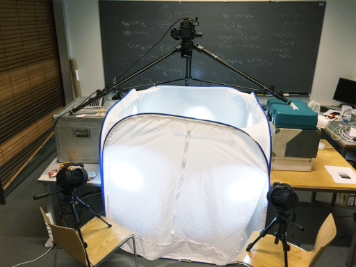 Figure 1
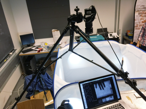 Figure 2
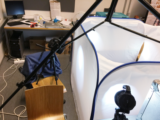 Figure 3
 Figure 4
 Figure 5
 Figure 6
 Figure 7
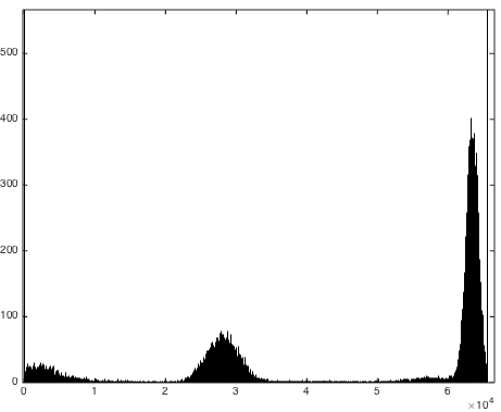 Figure 8
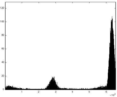 Figure 9
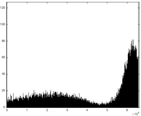 Figure 10
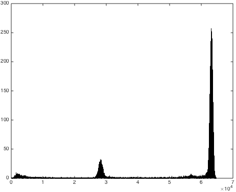 Figure 11
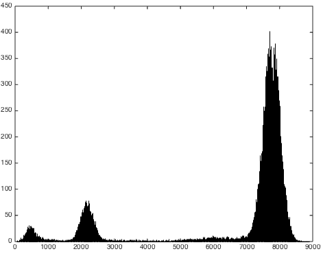 Figure 12
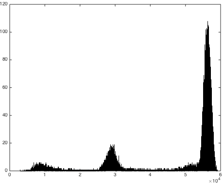 Figure 13
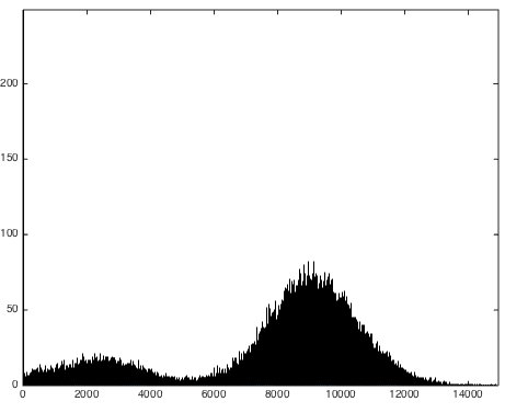 Figure 14
 Figure 15
 Figure 16
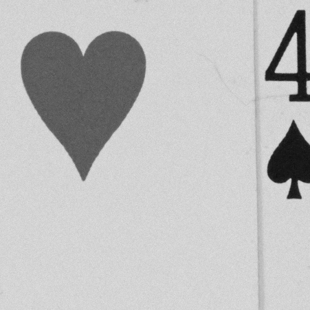 Figure 17
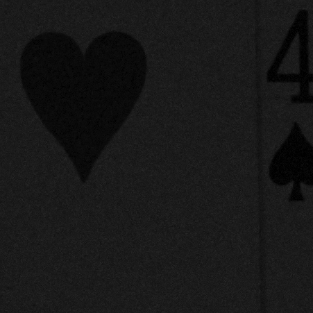 Figure 18
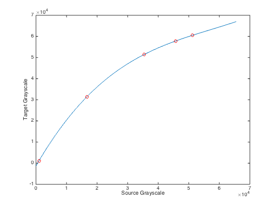 Figure 19
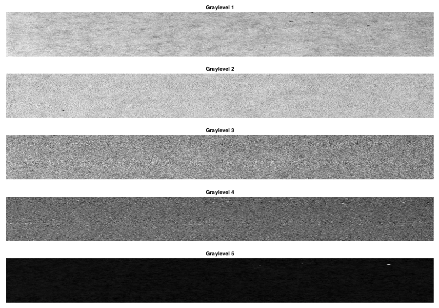 Figure 20
 Figure 21
 Figure 22
 Figure 23
 Figure 24
 Figure 25
 Figure 26
Peer Reviews
No public reviews on file for this paper yet. If you reviewed it on a platform where reviews are public (OpenReview, ICLR, NeurIPS, ICML), you can paste yours below so the community can read it here.
Videos
No videos yet. Explain this paper in a talk, walkthrough, or lecture? Add one.
Taxonomy
TopicsAdvanced Image and Video Retrieval Techniques · Image Retrieval and Classification Techniques
Photographic dataset: playing cards
Teemu Helenius, Santeri Kaupinmäki, Samuli Siltanen and David Villacis
Abstract.
A photographic dataset is collected for testing image processing algorithms.
Contents
1. Introduction
This document reports the acquisition, structure and properties of a digital photographic dataset collected at the Industrial Mathematics Laboratory of the Department of Mathematics and Statistics of University of Helsinki, Finland.
This dataset is designed to test and benchmark several image processing tasks, including: image denoising, image inpainting, etc., under the presence of real noise. This dataset is built with the goal of helping researchers in image processing and related areas to avoid the use of synthetic generated noise and blur to provide benchmarks and objective results.
2. Materials and Methods
2.1. Camera equipment
We use a PhaseOne XF medium-format camera equipped with an achromatic IQ260 digital back. The lens is Phase One Digital AF 120mm F4. The pixel size in the resulting 16bit TIFF image file is .
2.2. Lighting
The targets were lit with five Olight X6 Marauder LED flashlights with luminous flux of 5000 lm (nominal value, 4825 lm was measured in the laboratory of the vendor www.valostore.fi). The lights were positioned at roughly equiangular arrangement. The distance of each light from the target was roughly 850 mm. The lights were heating up quickly as they were used at maximum power. Cooling was enhanced with three regular household fans.
A diffuser was placed between the lights and the target to make the lighting more uniform and to reduce sharp shadows.
See Figure 1 for the imaging setup.
2.3. Details of the target
We placed playing cards on a horizontal surface. The camera was aimed directly down, so the optical axis was roughly vertical.
In every picture there is a five-step grayscale target for calibration.
2.4. Varying the noise level in the data
For each arrangement of cards, four different images were taken:
- (1)
Best-quality photo (im_clean.tif). Minimum ISO setting 200 and histogram approximately spanning the full dynamic range. The noise level is very small. 2. (2)
Medium-quality photo, first type (im_noise1.tif). Minimum ISO setting 200 and histogram approximately spanning a quarter the full dynamic range. This will introduce round-off errors from the AD converter. 3. (3)
Medium-quality photo, second type (im_noise2.tif). Maximum ISO setting 3200 and histogram approximately spanning the full dynamic range. This will introduce photon-counting noise as well as some electronic noise. 4. (4)
Low-quality photo (im_noise3.tif). Maximum ISO setting 3200 and histogram approximately spanning a quarter of the full dynamic range. The noise will be increased by added round-off errors.
3. Calibration
Due to the fact that the camera used in the acquisition process was using different parameters for different images, these images will have a different contrast and intensity values. In this section we will explain the techniques used to make the images have a common dynamic range and a similar histogram to the best-quality photo.
3.1. Intensity Adjustment
In this process we are interested in transforming the original image in such a way it maintains its structure while spreading the dynamic range of the image across a defined domain.
In order to define the grayscale levels we will make use of a grayscale calibration patch (phantom) that will be included in every image. The first step taken by the code is to extract the five graylevel areas as shown in Figure 2 and average the intensity values of the pixels inside it. This information is later used to build a non linear map by using a cubic spline interpolation of these graylevel calibration points, we can see an example of this mapping in Figure 3.
3.2. Histogram Matching
This procedure transforms the histogram of a givem image and a reference image and produces a modified image such that the histograms of the images and are similar. If we consider the graylevels in an interval , and let and denote the intensity levels for the input and output image respectively. The input levels have a probability density function and the output levels have the specified probability density function . A summary of the changes in the histogram of the dataset images cane be found in Figure 4
4. Results
The lens-target distance was approximately 120 cm. The image sensor was roughly parallel with the surface of the object layer. The aperture f-stop was f/11 in all of the shots.
Using this non linear map described in Section 3, we can adjust the intensity values and histogram of the images acquired using different setup configurations, and they all will present a similar dynamic range and histogram, as an example we can see a set of raw images and it corresponding adjustment in Figure 5 and a set of corrected images in Figure 6.
5. Discussion
This dataset enables us to analyze the denoising task given a real world kind of noise. We can test this work with the most popular denoising models like ROF [4] and TV-l1 [3], and see its performance under real world noise conditions. Let’s remember that these models make assumptions of the noise distribution, gaussian and poisson distribution for ROF and TV-l1 respectively.
In Figure 7, Figure 8 and Figure 9 we can see the output from applying a ROF denoising model to type 1, 2 and 3 noise type respectively. In this experiment we used FISTA [1] algorithm to find its numerical solution. Let’s recall that the ROF problem is given by:
[TABLE]
where is the given noisy image and is a finite difference operator used to obtain the Total Variation norm.
In Figure 10, Figure 11 and Figure 12 we can see the output from applying a TV-l1 denoising model to type 1, 2 and 3 noise type respectively. In this experiment we used a Primal-Dual algorithm described in [2] algorithm to find its numerical solution. Let’s recall that the TV-l1 model is given by:
[TABLE]
where is the given noisy image and is a finite difference operator used to obtain the Total Variation norm.
The reference list from the paper itself. Each links out to its DOI / PubMed record.
- 1[1] A. Beck and M. Teboulle , A Fast Iterative Shrinkage-Thresholding Algorithm for Linear Inverse Problems , SIAM Journal on Imaging Sciences, 2 (2009), pp. 183–202.
- 2[2] A. Chambolle, V. Caselles, D. Cremers, M. Novaga, and T. Pock , An introduction to total variation for image analysis , Theoretical foundations and numerical methods for sparse recovery, 9 (2010), pp. 263–340.
- 3[3] M. Nikolova , A Variational Approach to Remove Outliers and Impulse Noise , in Journal of Mathematical Imaging and Vision, vol. 20, 2004, pp. 99–120.
- 4[4] L. I. Rudin, S. Osher, and E. Fatemi , Nonlinear total variation based noise removal algorithms , Physica D: Nonlinear Phenomena, 60 (1992), pp. 259 – 268.