This paper introduces multi-colour partition algebras and bubble algebras, providing techniques to analyze their structure at roots of unity, especially in non-semisimple cases, advancing algebraic understanding.
Contribution
The paper defines new multi-colour partition and bubble algebras and develops methods to determine their structure over complex numbers at roots of unity.
Findings
01
Defined multi-colour partition algebras and bubble algebras.
02
Developed techniques for structural analysis in non-semisimple cases.
03
Extended understanding of algebraic properties at roots of unity.
Abstract
We introduce multi-colour partition algebras Pn,m(δ0,...,δm−1), which are generalization of both bubble algebras and partition algebras, then define the bubble algebra Tn,m(δ0,...,δm−1) as a sub-algebra of the algebra Pn,m(δ0,...,δm−1). We present general techniques to determine the structure of the bubble algebra over the complex field in the non-semisimple case.
\displaystyle\left.\begin{array}[]{r@{\mskip\thickmuskip}l}\mathfrak{S}_{n,m}\mskip 5.0mu plus 5.0mu&=\{d\in\mathcal{P}_{n,m}\mid\#(d)=n\},\\
\mathcal{A}_{n,m}\mskip 5.0mu plus 5.0mu&=\{d\in\mathcal{P}_{n,m}\mid d\text{ is planar}\},\\
\mathcal{B}_{n,m}\mskip 5.0mu plus 5.0mu&=\{d\in\mathcal{P}_{n,m}\mid\,\text{all blocks of }d\text{ have size }2\},\\
\mathcal{T}_{n,m}\mskip 5.0mu plus 5.0mu&=\mathcal{A}_{n,m}\cap\mathcal{B}_{n,m},\\
\widehat{\mathfrak{S}}_{n,m}\mskip 5.0mu plus 5.0mu&=\mathfrak{S}_{n,m}\cap\mathcal{A}_{n,m}.\end{array}\;\;\;\right\}
No public reviews on file for this paper yet. If you reviewed it on a platform where reviews are public (OpenReview, ICLR, NeurIPS, ICML), you can paste yours below so the community can read it here.
Videos
No videos yet. Explain this paper in a talk, walkthrough, or lecture? Add one.
Taxonomy
TopicsAlgebraic structures and combinatorial models · Advanced Combinatorial Mathematics · Advanced Topics in Algebra
Full text
The bubble algebras at roots of unity
Mufida M. Hmaida
Abstract. We introduce multi-colour partition algebras Pn,m(δ0,…,δm−1), which are generalization of both bubble algebras and partition algebras, then define the bubble algebra Tn,m(δ0,…,δm−1) as a sub-algebra of the algebra Pn,m(δ0,…,δm−1). We present general techniques to determine the structure of the bubble algebra over the complex field in the non-semisimple case.
1 Introduction
In 2003, Grimm and Martin[3] introduced a new construction, called the bubble algebra, this algebra defined entirely diagrammatically. They investigated its generic representations and proved that it is semi-simple when none of the parameters δi is a root of unity. Later, Jegan[4] showed that the bubble algebra is a cellular algebra in the sense of Graham and Lehrer[2], and that it is a tower of recollement when all of the δi are non-zero, as it is defined in [1] or [6]. The notion of a cellular algebra was first introduced by Graham and Lehrer [2]. Also Jegan[4] showed how certain idempotent sub-algebra of the bubble algebra corresponded to tensor products of the Temperley-Lieb algebras and investigated the homomorphisms between the cell modules of the algebra Tn,m(δ0,…,δm−1).
In this paper, we use a technique consist of reducing problems in the bubble algebra to problems in the Temperley-Lieb algebra. The representation theory of the Temperley-Lieb algebra is well known, see Martin [5], Ridout and Saint [7] and Westbury [8]. All the algebras in this paper are over the complex field and all the modules are left modules.
The main results of the paper are Theorems 8.2 and 8.3, which determine radical series of cell modules for the algebra Tn,m(δ0,…,δm−1) over the complex field and for all the tuples (δ0,…,δm−1) in case m=2 and m>2 respectively.
2 Preliminaries
For n∈N, the symbol Pn denotes the set of all partitions of the set n∪n′, where n={1,…,n} and n′={1′,…,n′}.
Each individual set partition can be represented by a graph, the graph is drawn in a rectangle with n nodes on the top row represent the elements in the set n and with n nodes on the bottom row of the rectangular represent the elements in the set n′, and the elements that in the same part at a partition, are represented as lines drawn connected their nodes inside the rectangular. Any diagrams are regarded as the same diagram if they representing the same partition.
Now the composition β∘α in Pn, where α,β∈Pn, is the partition obtained by placing α above β, identifying the bottom vertices of α with the top vertices of β, and ignoring any connected components that are isolated from boundaries. This product on Pn is associative and well-defined up to equivalence.
A (n1,n2)-partition diagram for any n1,n2∈N+ is a diagram representing a set partition of the set n1∪n2′ in the obvious way.
We can generalize the product on Pn to define a product of (n,m)-partition diagrams when it is defined: let α be (n1,n2)-diagram and β be (m1,m2)-diagram, β∘α is defined if and only if n2=m1 and it is (n1,m2)-diagram. For example, see the following figure.
∘= =
The diagrams representing partitions that spanning the Temperley-Lieb algebra TLn(δ) over (say) the complex field are planar (non-crossing) and their parts all have size two. Thus the following diagrams
are representing basis elements of the algebra TL4(δ).
We next briefly describe the cell modules of the algebra TLn(δ), which will be used in this paper.
A diagram representing a partition in the algebra TLn(δ) can be cut to construct a half-diagram such that all arcs on the top edge are above the cut, all arcs on the bottom edge are below the cut and each propagating line is only cut once. A half-diagram has p arcs called an (n,p)-link state. For example, the half-diagram
is a (7,3)-link state.
As the number of propagating lines can not increase by the multiplication, we can define left TLn-modules Mn,p which are spanned by (n,p′)-link states with p′≥p with action defined by putting the TLn(δ)-diagram above the half-diagram then proceeds as with TLn(δ) multiplication, and finally omit any new bottom arcs. Note that
[TABLE]
The Temperley-Lieb algebra is a cellular algebra, with the involution sending each diagram to its reflection in the horizontal plane, indexing set {0,1,…,[n/2]} and cell modules Vn,p:=Mn,p/Mn,p+1, see [2]. The dimension of Vn,p is (pn)−(p−1n):=dn,p. Note that (−1n)=0.
On each module Vn,p, there is a bilinear form ⟨,⟩n,p,δ defined as follows: if x and y are two (n,p)-link states, the scalar ⟨x,y⟩n,p,δ is computed by reflecting x in a horizontal axis and identifying its vertical border with that of y. The value ⟨x,y⟩n,p,δ is then non-zero only if every defect (an unconnected node) of x ends up being connected to one of y, and in this case ⟨x,y⟩n,p,δ=δl where l is the number of closed loops which is obtained from connecting x and y. For more details see section 9.5.2 in [5].
The matrix Gn,p,δ is defined to be the Gram matrix for the module Vn,p that represent the form ⟨,⟩n,p,δ with respect to a basis that contains all (n,p)-link states.
Let M be a module whose a bilinear form ⟨,⟩. The radical of this form on M is the set {x∈M∣⟨x,y⟩=0for all y∈M}. Define Rn,p,δ to be the radical of the previous bilinear form on the module Vn,p.
As we work over a field, the radical Rn,p is a sub-module of Vn,p. If δ=0, then Vn,p is cyclic and indecomposable. Moreover, Ln,p:=Vn,p/Rn,p is irreducible. The cell modules Vn,p of the algebra TLn(δ) are irreducible except for particular values of the scalar δ. Throughout this paper, let δ=q+q−1 with q∈C.
Proposition 2.1**.**
[5, Section 6.4, Theorem 1].
If q is not a root of unity, then the algebra TLn(δ) is semi-simple, and the modules Vn,p, where 0≤p≤[n/2], form a complete set of non-isomorphic irreducible modules of the algebra TLn(δ).
Let q be a root of unity and let l be the minimal positive integer satisfying q2l=1. The module Vn,p (or the pair (n,p)) is called critical if q2(n−2p+1)=1.
Theorem 2.2**.**
[5, Section 7.3, Theorem 2].
If 0≤p1−p2<l and n−p1−p2+1=0(modl), then there is a non-trivial homomorphism θ:Vn,p2→Vn,p1. Furthermore, the kernels and co-kernels of the homomorphism θ are irreducible. Otherwise, there is no non-trivial homomorphism from Vn,p2 to Vn,p1.
Define r(n,p) be the integer satisfying the equation n−2p+1=kl+r(n,p), where k∈N and r(n,p)∈{1,…,l}. The critically of (n,p) is equivalent to r(n,p)=l.
Proposition 2.3**.**
[5, Section 7.3, Theorem 2].
Let q be a root of unity and (n,p) be non-critical. Then
[TABLE]
3 The bubble algebra Tn,m(δ0,…,δm−1)
Throughout the paper, let n,m be positive integers, C0,…,Cm−1 be different colours where none of them is white, and δ0,…,δm−1 be scalars corresponding to these colours.
The aim of this section is introducing the multi-colour partition algebra and then defining the bubble algebra as a sub-algebra.
Define the set Φn,m to be
[TABLE]
We construct basis elements of the multi-colour partition algebra in similar way of the algebra Pn(δ). Let (A0,…,Am−1)∈Φn,m (note that some of these subsets can be an empty set). Define PA0,…,Am−1 to be the set ∏i=0m−1PAi, where PAi is the set of all partitions of Ai, and
[TABLE]
The element d=(d0,…,dm−1)∈∏i=0m−1PAi can be represented by the same diagram of the partition ∪i=0m−1di∈Pn after colouring it as follows: we use the colour Ci to draw all the edges and the nodes in the partition di.
A diagram represents an element in Pn,m is not unique. We say two diagrams are equivalent if they represent the same tuple of partitions. The term multi-colour partition diagram will be used to mean an equivalence class of a given diagram. For example, the following diagrams
are equivalent.
We define the following sets for each element d∈∏PAi:
[TABLE]
Definition 3.1**.**
Let Pn,m(δ0,…,δm−1) be C-vector space with the basis Pn,m and with the composition:
[TABLE]
where δi∈C, α,β∈Pn,m, ci is the number of removed connected components from the middle row when computing the product βi∘αi for each i=0,…,m−1 and ∘ is the normal composition of partition diagrams.
Proposition 3.2**.**
The product on Pn,m(δ0,…,δm−1) that defined in the previous definition, is associative.
Proof.
Let α=(αi),β=(βi) and ρ=(ρi) be multi-colour partitions in Pn,m.
Note that top(αi∘βi)=top(βi) and bot(αi∘βi)=bot(αi) as long as α∘β is defined. From the multiplication on Pn,m, the composition α∘(β∘ρ) is defined if and only if top(αi)=bot(βi∘ρi) for each i, and β∘ρ is defined if and only if top(βi)=bot(ρi) for each i. But if β∘ρ is defined then bot(βi∘ρi)=bot(βi) for each i. Then α∘(β∘ρ) is defined if and only if top(αi)=bot(βi) and top(βi)=bot(ρi) for each i. Similarly, (α∘β)∘ρ is defined if and only if top(αi)=bot(βi) and top(βi)=bot(ρi) for each i. So the composition α∘(β∘ρ) is defined if and only if (α∘β)∘ρ is defined, then the product in Pn,m(δ0,…,δm−1) is an associative when vanishes.
Furthermore, if it does not vanish, we have
[TABLE]
as the composition of partition diagrams is associative.
∎
From the previous proposition, we have Pn,m(δ0,…,δm−1) is an associative algebra with identity:
[TABLE]
where Ξn,m:={(A0,…,Am−1)∣∪i=0m−1Ai=n,Ai∩Aj=∅∀i=j}, 1Ai is the partition of the set Ai∪Ai′ where any node j is only connected with the node j′ for all j∈Ai and Ai′={j′∣j∈Ai}, for all 0≤i≤m−1. This means the identity is the summation of all the different multi-colour partitions that their diagrams connect i only to i′ with any colour for each 1≤i≤n. The algebra Pn,m(δ0,…,δm−1) is called the multi-colour partition algebra.
Definition 3.3**.**
[3, Section 2].
The propagating number of α∈Pn,m, #(α), is the number of parts which contain nodes from both the top and the bottom rows in any colour, i.e. #(α)=∑i=0m−1#(αi) or simply \#(\alpha)=\#\big{(}\cup_{i=0}^{m-1}\alpha_{i}\big{)}.
Definition 3.4**.**
[3, Section 2].
The Cj- propagating number of α∈Pn,m, #j(α), is the propagating number of αj.
The propagating number of diagrams in the algebra Pn,m has similar property of propagating number of diagrams in Pn(δ): if α,β∈Pn,m with αβ=0, then
[TABLE]
A planar multi-colour partition in the set Pn,m is a multi-colour partition whose a diagram that does not have edge crossings in the same colour. This is the same definition that Grimm and Martin use in [3]. In other words, there can be crossed edges but they don’t have the same colour. This definition of planar diagram is consistent with the definition of planar diagram in the algebra Pn(δ) provided that considering all the diagrams in Pn(δ) have been coloured by using only one colour.
We define subsets of Pn,m corresponding to those subsets of Pn, as following:
[TABLE]
The diagrams in the bubble algebra, as Grimm and Martin[3] defined them, in the case of two colours can be constructed by drawing two Kauffman diagrams (or just one) with no internal loops, using different colours in the same frame with n nodes on the northern face and n nodes on the southern face, such that if a node is contained in first Kauffman diagram, it will not be contained in the second. This means that at these diagrams the nodes are connected in pairs with different colours where an intersection is just allowed between different colour edges.
The bubble algebra Tn,m(δ0,…,δm−1) (it is denoted by Tn2(δr,δb) in [3] in the case of two colours), or simply Tn,m and Tn,m(δ˘) for simplicity where δ˘=(δ0,…,δm−1), is the C-linear extension of the set of isotopy classes of previous diagrams and composition defined as the one on Pn,m(δ0,…,δm−1), with internal closed loop replacement. The loop replacement scalar here depends on the colour.
Theorem 3.5**.**
The bubble algebra Tn,m(δ0,…,δm−1) is the sub-algebra of the algebra Pn,m(δ0,…,δm−1) spanned by the set Tn,m, which is defined in equation (9).
Proof.
From the description of diagrams in the bubble algebra Tn,m(δ0,…,δm−1), we can identify bubble diagrams with multi-colour partitions and hence define it as sub-algebra of the algebra Pn,m(δ0,…,δm−1). We are going to show that Tn,m is closed under the composition on Pn,m and then the rest follows immediately from the algebra Pn,m and from bubble diagrams realisation and from the fact 1(A0,…,Am−1)∈Tn,m for each (A0,…,Am−1)∈Ξn,m. Let D=(D0,…,Dm−1) and B=(B0,…,Bm−1) be multi-colour partitions in Tn,m such that BD=0, so we have Di∘Bi is defined as partition diagrams. Now from the definition of Tn,m, all the partitions Di and Bi are representing by Kauffman diagrams, but then Di∘Bi is also representing by Kauffman’s diagram for each i, and we are done.
∎
4 Cell modules
Making an arc, an edge connects two nodes in the same row (top or bottom) of a diagram, needs two vertices on this row, so the propagating number of any diagram d∈Tn,m has the form #(d)=n−2v for some integer v, where 0≤v≤[n/2].
Define the set Γ(l,m) to be
[TABLE]
and the set
[TABLE]
We follow Grimm and Martin [3] and define the subset Tn,m[λ0,…,λm−1], or simply Tn,m[λ], to be {d∈Tn,m∣#j(d)=λj for allj∈Zm}, where λ∈Λ.
A half-multi-colour diagram, or simply half-diagram, is a diagram obtained by cutting horizontally a diagram in the set Tn,m in the middle such that each propagating line is cut once, thus this is well defined on classes. As for the Temperley-Lieb algebra, we can form a unique bubble algebra diagram from two half-diagrams providing that they have the same number of propagating lines of each colour. Let Tn,m∣⟩[λ] be the set of top pieces obtained by cutting elements of the set Tn,m[λ], where λ∈Λ. Similarly Tn,m⟨∣[λ] is the set of bottom pieces obtained by cutting elements of Tn,m[λ].
A half-diagram is called a ((n0,p0),…,(nm−1,pm−1))-link state, if it contains both nj nodes and pj arcs of the colour Cj for each j. This means that there are nj−2pj unconnected nodes of the colour Cj for each j.
Denote by CMn(λ0,…,λm−1), or simply CMn(λ) where λ∈Λ, the vector space with a basis Mn(λ) which contains all link states that have number of defects of the colour Cj on the form λj−2tj for each j∈Zm where 0≤tj≤[λj/2]. Note that there is no condition on the colours of arcs.
Lemma 4.1**.**
Let λ∈Λ. The vector space CMn(λ) is a left Tn,m- module with the action defined by the concatenation of diagram with a half-diagram then proceeding as we would with two diagrams in Tn,m (remove each loop and replace it by parameter corresponding to the loop’s colour and it will be zero if they have different distribution of colours), and finally omit any new bottom arcs.
Proof.
Let x∈Tn,m and d be a half-diagram in Mn(λ). Without loss of generality, we can assume xd=0, multiplying x with d can not create any additional propagating lines of any colour. Thus the number of Cj-defects in xd is of the form λj−2tj where 0≤tj≤[λj/2], because making an extra Cj-arc needs two Cj-nodes.
∎
Define a subset Mn<(λ) to be ⋃j=0m−1Mn(λ0,…,λj−2,…,λm−1). Note that Mn(λ0,…,λj−2,…,λm−1) is taken to be the empty-set when λj<2. Let CMn<(λ) be the module that generated by Mn<(λ), thus CMn<(λ) is a sub-module of CMn(λ).
Lemma 4.2**.**
Let Δn(λ) be the module CMn(λ)/CMn<(λ) of Tn,m, where λ∈Λ. Then the module Δn(λ) has the set Tn,m∣⟩[λ] as a basis.
Proof.
The quotient CMn(λ)/CMn<(λ) sends any link state with less than λj defects of the colour Cj for each j to be zero. Thus the left multiplication by any diagram in the set Tn,m will be either zero or a half-diagram in Tn,m∣⟩[λ].
∎
5 Cellularity of the bubble algebra
Theorem 5.1**.**
[4, Proposition 1.3.2].
The algebra Tn,m(δ˘) is cellular over any field, with the involution sending each diagram to its reflection in the horizontal plane, and the indexing set Λ=⋃v=0[n/2]Γ(n−2v,m). The order on the set Λ is defined by
λ≥λ′* f and only if λj≤λj′ for each j.*
The modules Δn(λ) where λ∈Λ are cell modules of the algebra Tn,m.
Each cell module Δn(λ) comes with a contravariant inner product via its basis of top half-diagrams, defined as follows: let d,d′∈Tn,m[λ], x=⟨d∣ and y=∣d′⟩, so
[TABLE]
so \langle x,y\rangle=\left\{\begin{array}[]{ll}\langle d||d^{\prime}\rangle&\text{ if}\;d^{\prime\prime}\in\mathcal{T}_{n,m}[\lambda],\\
0&\text{otherwise}.\end{array}\right.
Let Gn(λ) to be the Gram matrix of the previous inner product on the cell module Δn(λ) with respect to half-diagrams basis. Since we work over a field, we can check when the module Δn(λ) is simple by computing detGn(λ) as long as ⟨,⟩=0. Grimm and Martin [3] showed that the cell modules Δn(λ0,λ1) are generically simple.
Let Λ0 be subset of Λ that contains all λ∈Λ such that ⟨,⟩=0. Note that when δj=0 for some j, then Λ0=Λ, since we can take a half diagram with all the arcs of the colours corresponding to non-zero scalars. Even if δj=0 for all j, then for each cell module Δn(λ) with ∑j=0m−1λj=0, the inner product ⟨,⟩=0 because we can still find diagrams such their product is equal to one. Thus Λ0=Λ unless n is an even integer and δi=0 for each i∈Zm. In the case n is an even integer and δi=0 for each i∈Zm, then Λ0=Λ∖{(0,…,0)}. Then the bubble algebra Tn,m(δ˘) is a quasi-hereditary if and only if δj=0 for some 0≤j<m or n is an odd integer.
Let Tn,2+(δ˘) be the subspace of Tn,2(δ˘) that spanned by all the diagrams in Tn,2 which have an even number of blue-nodes on the top face. Since making an arc needs two nodes on the same face, thus the number of blue-nodes on the bottom face of the diagrams in Tn,2+(δ˘) will be also an even number. The composition of two diagrams in Tn,2(δ˘) does not change the number of blue-nodes on top face of the first diagram, thus Tn,2+(δ˘) is an algebra with an identity equals to the sum of all coloured images of id∈Sn that have an even number of blue-propagating lines. Similarly, define Tn,2−(δ˘) to be the subspace of Tn,2(δ˘) that spanned by all the diagrams in Tn,2 which have an odd number of blue-nodes on the top face. Also, Tn,2−(δ˘) is an algebra with identity equals to the sum of all coloured image of id∈Sn that have an odd number of blue-propagating lines.
Lemma 5.2**.**
For any n>0, we have Tn,2(δ˘)=Tn,2+(δ˘)⊕Tn,2−(δ˘), as algebra.
Proof.
This come from the fact any diagram in Tn,2 will have even number or odd number of blue-nodes on the top face, so Tn,2(δ˘)=Tn,2+(δ˘)+Tn,2−(δ˘). Furthermore, it is clear that Tn,2+(δ˘)∩Tn,2−(δ˘) is zero and the product of any two elements from Tn,2+(δ˘) and Tn,2−(δ˘) will be zero.
∎
As consequence of last lemma, to study the representations of the algebra Tn,2(δ˘), it is enough to study the representations of the algebras Tn,2+(δ˘) and Tn,2−(δ˘).
6 Idempotent Localisations
Let μ∈Γ(n,m), we define μ to be
[TABLE]
Proposition 6.1**.**
Let (Ai)∈Ξn,m and #j(1(Ai))=μj for each j, then the elements 1(Ai) and 1μ are conjugate in the algebras Tn,m and Pn,m.
Proof.
To show that we need to define an invertible element D∈Tn,m such that D−11(Ai)D=1μ. Claim that the element
[TABLE]
satisfies the previous equation, where θ(Ai) is the multi-colour partition obtained from colouring a permutation θ with top equals (Ai), and θ is specific permutation changes the order of coloured lines without crossing lines that have the same colour.
Lets define the map θ∈Sn as follows: assume that i∈n and i∈Aj, and define θ(i) to be νi,j+k<j∑μk, where νi,j be the number of integers l∈n that smaller than i and l∈Aj.
We are going to show that θ∈Sn, by proving that θ is an injective map. It is obvious that θ is well-defined. Assume that i1,i2∈n without loss of generality we can say that i1<i2. Now there are two probabilities, i1,i2∈Aj or i1∈Aj1=Aj2∋i2. If i1,i2∈Aj for some j, then νi1,j<νi2,j so θ(i1)<θ(i2). On the other side when j1=j2, if j1<j2, so θ(i1)=νi1,j1+k<j1∑μk≤k<j1+1∑μk<θ(i2). Similarly, if j2<j1, thus θ(i2)<θ(i1). Therefore θ is an injective.
From the way that we define θ, it is evidential that θ(Ai)∈Tn,m since if i,j∈Ah for some h where i<j, so θ(i)<θ(j) this implies that there is no crossing lines with same colour. Similarly, the diagram \big{(}\theta^{-1}\big{)}_{(A_{i})}, the coloured image of θ−1 with bottom equals (Ai), is contained in Tn,m because by flipping the diagram \big{(}\theta^{-1}\big{)}_{(A_{i})} we obtain θ(Ai). Also note that bot(θ(Ai))=μ.
Finally, take D=θ(Ai)+B∈Ξn,m∖{(Ai)}∑1B and D^{\prime}=\big{(}\theta^{-1}\big{)}_{(A_{i})}+\sum\limits_{B\in\Xi^{n,m}\setminus\{\underline{\mu}\}}1_{B}. Note that D,D′∈Tn,m, DD′=1Tn,m=D′D and D1(Ai)D′=1μ.
∎
Jegan[4] proved in Theorem 3.1.4, for any μ∈Γ(n,m) the algebras ⨂i=0m−1TLμi(δi) and 1μTn,m(δ˘)1μ are isomorphic with a map sending any tuple of diagrams in the algebra ⨂i=0m−1TLμi(δi) to the diagram in 1μTn,m(δ˘)1μ formed by drawing these diagrams in one frame one by one using different colours such that the diagram from TLμi(δi) is drawn in the colour Ci. Similarly, if Vμ0,p0,…,Vμm−1,pm−1 are cell modules for the algebras TLμ0(δ0),…,TLμm−1(δm−1) respectively, then elements of the module ⨂i=0m−1Vμi,pi can be represented by \big{(}(\mu_{i},p_{i})\big{)}_{i\in\mathbb{Z}_{m}}- link states, see Figure 1, by using the same map which it is the same isomorphism that Jegan used in the proof of the fact: let λ∈Λ and μ∈Γ(n,m), then
[TABLE]
as 1μTn,m1μ-module.
Important convention : whenever i=0⨂m−1Vμi,pi or i=0⨂m−1Mi are mentioned, where Mi is a sub-module or quotient module of Vμi,pi, we mean their image in 1μΔn(λ) under the previous isomorphism.
A basis of Δn(λ) is the set that contains all \big{(}(\lambda_{j}+2p_{j},p_{j})\big{)}_{j\in\mathbb{Z}_{m}}-link states where p0,…,pm−1 are non-negative integers such that ∑j∈Zm(λj+2pj)=n, which is the same as the basis Tn,m∣⟩[λ]. Each \big{(}(n_{j},p_{j})\big{)}_{j\in\mathbb{Z}_{m}}-link state determines a collection of (nj,pj)-link states as they are defined in Section 2, where each j represents the colour Cj, by omitting all the parts that have colour not Cj, thus
[TABLE]
where λ∈Γ(n−2v,m). For example, take α to be the ((3,1),(2,0),(4,1))-link state , so α can be consider as a collection of the next link states:
Let a=∣D⟩∈Δn(λ) for some D∈Tn,m[λ]. The distribution of the colours of a is the set top(D). This set will be denoted by top(a).
Let a be a \big{(}(\lambda_{j}+2p_{j},p_{j})\big{)}_{j\in\mathbb{Z}_{m}}-link state and b be a \big{(}(\lambda_{j}+2p^{\prime}_{j},p^{\prime}_{j})\big{)}_{j\in\mathbb{Z}_{m}}-link state where ∑j∈Zmpj=∑j∈Zmpj′. It is evident that ⟨a,b⟩=0 unless pj=pj′ for each j and the distributions of the colours of a and b are same. When pj=pj′ for each j and top(a)=top(b), and aj be the (nj,pj)-link state which is obtained from a by omitting all the parts that have colour not Cj. Similarly, we define bj. From the graphical visualization of the product on the algebra Tn,m, we obtain
[TABLE]
where ⟨aj,bj⟩nj,pj,δj denotes the standard bilinear form on Vnj,pj as TLnj(δj)-module. Note that distribution of colours, if it matches up, does not play any rule. In other words, if a,b,c and d be \big{(}(n_{j},p_{j})\big{)}_{j\in\mathbb{Z}_{m}}-link states such that aj=cj and bj=dj, then ⟨a,b⟩=⟨c,d⟩ if top(a)=top(b) and top(c)=top(d). Note that a and c may have different distributions of colours. As consequence of this, we have the following theorem.
Theorem 6.2**.**
[4, lemma 3.2.10].
If ∑j∈Zmλj=n−2v for some v, then the Gram matrix of the cell module Δn(λ) of the previous inner product with respect to half-diagrams basis can be written in the form
[TABLE]
where Gλj+2uj,uj,δj is the Gram matrix of the cell TLλj+2uj(δj)-module Vλj+2uj,uj with a specific bilinear form and half-diagrams basis. Therefore, the determinant of Gram matrix is
[TABLE]
where dλj+2uj,uj=dimVλj+2uj,uj and nμ:=(μ0,…,μm−1n) for each μ∈Γ(n,m).
∎
If ∑jλj=n, from the last theorem we have Gn(λ)=⨁nλ(1)=Inλ×nλ, where Inλ×nλ is the identity matrix, so the module Δn(λ) is simple whenever ∑jλj=n. Also, if δj=qj+qj−1=0 for all j∈Zm and qj is not a root of unity for any j, then the algebra Tn,m(δ˘) is semi-simple.
Proposition 6.3**.**
Let λ∈Λ0. The head of the module Δn(λ) where λ∈Γ(n−2v,m) for some v, denoted by Ln(λ), satisfy the relation
[TABLE]
where Lλi+2ui,ui,δi is the head of the TLλi+2ui(δi)-module Vλi+2ui,ui.
Proof.
This follows from the fact that dimLn(λ)=rank(Gn(λ)) since our algebra is over a field and by using Theorem 6.2 and properties of the rank of matrices.
∎
Corollary 6.4**.**
Let λ∈Λ0. The module Ln(λ) decomposes as
[TABLE]
as a vector space, where λ∈Γ(n−2v,m) for some v.
Proof.
It comes directly from the fact that any two vector spaces have the same dimension they are isomorphic.
∎
Lemma 6.5**.**
The dimensions of Rad(Δn(λ0,λ1)), the radical of Δn(λ0,λ1), is
[TABLE]
where λ∈Γ(n−2v,2) and Rλi+2ui,ui,δi is the radical of the TLλi+2ui(δi)-module Vλi+2ui,ui.
Proof.
Since dimRad(Δn(λ))=dimΔn(λ)−dimLn(λ), so dimRad(Δn(λ)) equals
[TABLE]
But dimLn,p,δ=dimVn,p−dimRn,p,δ, so dimRad(Δn(λ)) is
[TABLE]
Theorem 6.6**.**
Let λ∈Γ(n−2v,2) for some v. Then Rad(Δn(λ0,λ1)) decomposes as
[TABLE]
as a vector space, and it is equal to
[TABLE]
Remember by Rλ0+2u0,u0,δ0⊗Vλ1+2u1,u1 and Vλ0+2u0,u0⊗Rλ1+2u1,u1,δ1 we mean their images in the module 1λ+2uΔn(λ).
Proof.
First part comes directly from last lemma, since they have the same dimension, note that
[TABLE]
Now we are going to prove the second part. As we mentioned before we have
[TABLE]
Let y be a ((λ0+2u0′,u0′),(λ1+2u1′,u1′))-link state for some u′∈Γ(v,2), so from the last equation we can assume that y=π(y0⊗y1) for some π∈Sn,2 and yi is a (λi+2ui′,ui′)-link state for each i, and let x be an element in \sigma\big{(}\,\mathsf{R}_{\lambda_{0}+2u_{0},u_{0},\delta_{0}}\otimes\mathsf{V}_{\lambda_{1}+2u_{1},u_{1}}\,\big{)} or in \sigma\big{(}\,\mathsf{V}_{\lambda_{0}+2u_{0},u_{0}}\otimes\mathsf{R}_{\lambda_{1}+2u_{1},u_{1},\delta_{1}}\,\big{)} for some u∈Γ(v,2) and some σ∈Sn,2, so we can assume that x=σ(x0⊗x1) where x0∈Rλ0+2u0,u0,δ0 or x1∈Rλ1+2u1,u1,δ1. If u=u′ or σ=π, this means the colour distributions of x and y are different, so from the definition of the multiplication on the algebra Tn,m we have ⟨y,x⟩=0. On the other hand, if u=u′ and σ=π, from equation (10) we have ⟨y,x⟩=⟨y0,x0⟩λ0+2u0,u0,δ0⟨y1,x1⟩λ1+2u1,u1,δ1. But xi∈Rλi+2ui,ui,δi for some i, so ⟨yi,xi⟩λi+2ui,ui,δi=0 for some i. Hence ⟨y,x⟩=0 for each y∈Δn(λ), which means x∈Rad(Δn(λ)). Thus
[TABLE]
but both of them have the same dimension thus they are identical.
∎
Theorem 6.7**.**
Let λ∈Γ(n−2v,m) for some v. Then the radical Rad(Δn(λ)) equals
[TABLE]
Remember by the tensor product of the modules in the last equation we mean their images in the module 1λ+2uΔn(λ).
Proof.
We can show that by using induction on m and Theorem 6.6.
∎
Corollary 6.8**.**
Let λ∈Γ(n−2v,m), then
[TABLE]
By ⊗i=0m−1Lλi+2ui,ui,δi we mean its images in the module 1λ+2uΔn(λ).
Proof.
From the definition of the head of cell module over a field and from the last theorem, we have Ln(λ) equals
[TABLE]
where we put Ri:=Rλi+2ui,ui,δi and Vi:=Vλi+2ui,ui for simplicity. Let xi∈Lλi+2ui,ui,δi:=Li for each i, so xi=ai+Ri for some ai∈Vi and from that we have
[TABLE]
it follows that
[TABLE]
for each u∈Γ(v,m). We are done
∎
7 Homomorphisms between cell Tn,m-modules
As we said, the algebra Tn,m(δ˘) is semi-simple algebra when qj is not root of unity where δj=qj+qj−1=0 for each j∈Zm. Therefore in what follows, it will be assumed that qj is a root of unity for some j, and let lj be the minimal positive integer satisfying qj2lj=1.
The first part of next proposition is Lemma 4.1.1 in [4].
Proposition 7.1**.**
Let λ,μ∈ΛTn,m and θ:Δn(λ)→Δn(μ) be a homomorphism defined by θ(a)=∑iαibi, where αi∈C, a∈Tn,m∣⟩[λ] and bi∈Tn,m∣⟩[μ] for each i. Then the following are true:
top(a)=top(bi)* for each i.*
2. 2.
μj=λj−2tj, for some tj∈{0,…,[λj/2]}.
3. 3.
If δj is invertible and a contains an Cj-arc, then bi contains an Cj-arc in the same position. This means that θ preserves arcs when δj=0 for each j∈Zm.
Proof.
We are going to show only the last part. Assume that a contains h arcs of the colour Cj and δj=0. Take x∈Tn,m to be the diagram defined as follows: top(x)=bot(x)=top(a) and if any two nodes k,l∈n are connected in a by a Cj-arc, then these nodes will be also connected in x by a Cj-arc and k′,l′ will be connected by the same colour, other that all the nodes will be connected to their projection in the bottom row. Note that xa=δjha, so
[TABLE]
The Cj-arcs on the top row will not be affected by the product, so they will be in xbi in the same positions of a for each i.
∎
Let λ∈Γ(n−2v,m) for some v, and θ:Δn(λ)→Δn(λ−2t) be a homomorphism, where λ−2t=(λ0−2t0,…,λm−1−2tm−1). The homomorphism θ will be non-zero if and only if there is μ∈Γ(n,m) of the form μ=λ+2p for some p∈Γ(v,m) such that θ(1μΔn(λ))={0}. Thus we can restrict θ to define a non-trivial homomorphism
[TABLE]
Note that if δi=0 for each i, so p does not have any important role since it is corresponding to number of arcs which are actually preserved, see Proposition 7.1. Furthermore, if we have a homomorphism from ⊗i=0m−1Vλi+2pi,pi to ⊗i=0m−1Vλi+2pi,pi+ti, we can extend it to get a homomorphism from Δn(λ) to Δn(λ−2t). Thus
[TABLE]
if and only if
[TABLE]
for each p∈Γ(v,m).
Now, if there is a non-zero homomorphism fi∈HomTLμi(δi)(Vμi,pi,Vμi,pi+ti) for each i, then ⊗fi∈Hom⊗i=0m−1TLμi(δi)(⊗i=0m−1Vμi,pi,⊗i=0m−1Vμi,pi+ti) is also non-zero. From the previous details we have the following propositions.
Proposition 7.2**.**
[4, Theorem 6.2.2].
Let δj is invertible for each j, λ′=λ−2t where ∑j=0m−1λj=n−2v for some v. Suppose there exist non-zero homomorphisms from Vλi,0 to Vλi,ti as TLλi(δi)-modules for each i. Then there exists a non-trivial homomorphism from Δn(λ) to Δn(λ′).
8 The Cartan matrix of the bubble algebra
Throughout this section we assume that δi=qi+qi−1∈C for each i and at least one of the parameters is a root of unity other than ±1. We aim to compute the decomposition matrix of the algebra Tn,m over complex field, then the Cartan matrix for Tn,m can be found, since the bubble algebra is cellular.
Proposition 8.1**.**
Let λ∈Γ(n−2v,m) for some v. The module Δn(λ) is simple if and only if λi+1=0(modli) whenever qi is a root of unity where i∈Zm.
Proof.
If qi is not a root of unity for some i∈Zm, Proposition 2.1 implies to Lλi+2ui,ui,δi=Vλi+2ui,ui for any u∈Γ(v,m). On the other hand, if qi is a root of unity for some, recall that dimLni,ui,δi=dimVni,ui whenever ni−2ui+1=0(modli). Since (λi+2ui)−2ui+1=0(modli), so Lλi+2ui,ui,δi=Vλi+2ui,ui. Now, by substituting in equation (11), we obtain dimLn(λ)=dimΔn(λ), we are done.
∎
Next we are going to compute the Loewy length and Loewy layers for each cell module of the bubble algebra.
Theorem 8.2**.**
Let Tn,2(δ0,δ1) be the bubble algebra over the complex field and λ0+λ1=n−2v, λi+ti+1=0(modli) where i=0,1 and 0<ti<li, then
[TABLE]
is an exact sequence, where t=(t0,t1). Whenever x0+x1>n, we put Ln(x0,x1)={0} for any x0,x1∈N.
Proof.
Let Rui,i:=Rλi+2ui,ui,δi and Vui:=Vλi+2ui,ui. Define W1,W2 and W1,2 to be
[TABLE]
[TABLE]
Note that Rad(Δn(λ))=W1+W2, see Theorem 6.6, and W1,2=W1∩W2. To prove our theorem we are going to show that Ln(λ+2t)≅W1,2 and (W1+W2)/W1,2≅Ln(λ0+2t0,λ1)⊕Ln(λ0,λ1+2t1).
First, we need to show that W1 and W2 are sub-modules of the module Rad(Δn(λ)). This implies to W1,2 is also sub-module. Let x=σ(a0⊗a1)∈W1 where σ∈Sn,2, a0∈Ru0,0 and a1 is a link state in Vu1 for some u, and let D=(D0,D1)∈Tn,2. Since Rad(Δn(λ))=W1+W2, so x and Dx is also contained in Rad(Δn(λ)). Without losing the generality, we can assume Dx=0, then from the graphical visualization we have Dx=\zeta\big{(}(D^{\prime}_{0}a_{0})\otimes(D^{\prime}_{1}a_{1})\big{)} for some ζ∈Sn,2 and Di′ is the diagram Di after ignoring the colour, see next example. Note that there exists D1 such that D1′a1 will be not contained Ru1′,1 for some u1′ since δ1=0(as Vu1′=Ru1′,1), thus D0′a0∈Ru0′,0 for some u′∈Γ(v,2), from this we have Dx∈W1, this implies to W1 is a sub-module. Similarly, W2 is a sub-module of Rad(Δn(λ)).
From Theorem 2.2, there is an TLλi+2ui(δi)-isomorphism fui,i:Lui,i→Rui,i, where Lui,i:=Lλi+2ui,ui,δi, since λi+ti+1=0(modli) and 0<ti<li for each u∈Γ(v,2). By using one of these isomorphisms we can define a non-zero homomorphism from Ln(λ+2t) to W1,2 as follows: Fix u∈Γ(v,2) and fu0,0 and fu1,1. By using fu0,0 and fu1,1 we obtain an TLλ0+2u0(δ0)⊗TLλ1+2u1(δ1)-module isomorphism fu0,0⊗fu1,1 from Lu0,0⊗Lu1,1 to Ru0,0⊗Ru1,1. Hence we can define the map Ψ:Ln(λ+2t)→W1,2 to be the extension of fu0,0⊗fu1,1 as Ln(λ+2t)=∑w∈Γ(v,2)∑σ∈Sn,2σ(Lw0,0⊗Lw1,1). To prove that Ψ is a non-zero Tn,2-homomorphism, it is enough to show that Ψ is well-defined, i.e. if D(a0⊗a1)=0 where D∈Tn,2 and ai∈Lui,i for each i, then D(fu0,0(a0)⊗fu1,1(a1))=0. From the way we define Ru0,0⊗Ru1,1 and Lu0,0⊗Lu1,1, we have a0⊗a1 and fu0,0(a0)⊗fu1,1(a1) have the same top λ+2u, and since the set top(D) and the arcs in top half of D don’t have any effect on the product, so without losing the generality we can assume that D=D0⊗D1 where Di∈TLλi+2ui, but then every thing comes directly from the fact fu0,0⊗fu1,1 is an TLλ0+2u0(δ0)⊗TLλ1+2u1(δ1)- module isomorphism, hence Ψ is a non-zero homomorphism. Now as Ln(λ+2t) is simple module and the fact that they have the same dimension, finally by using the first isomorphism theorem we obtain that they are isomorphic.
Now since W1,2=W1∩W2, so (W1+W2)/W1,2≅W1/W1,2⊕W2/W1,2 . Also
[TABLE]
Now as we did to prove the isomorphism between W1,2 and Ln(λ+2t), we can show that u∈Γ(v,2)∑σ∈Sn,2∑σRu0,0⊗Lui,i≅Ln(λ0+2t0,λ1). Similarly, W2/W1,2≅Ln(λ0,λ1+2t1).
∎
Example 8.2.1**.**
*Let δ0=δ1=1. It is easy to show that −
is an element in R3,1,δ0, so the element −
is contained in Rad(Δ6(1,1)), since it is an element in \sigma\big{(}\mathsf{R}_{3,1,\delta_{0}}\otimes\mathsf{V}_{3,1}\big{)} for some σ∈S6,2. Also*
\Big{(}$$-
\Big{)}=
\Big{(}$$-
\Big{)},
*note that the element −
is an element in R5,2,δ0.*
Example 8.2.2**.**
Let δ˘=(0,2), then l0=2 and l1=4 and the critical lines are λ0=1,3,5,… and λ1=3,7,… which are represented by coloured lines in figure 2. Also the arrows in the figure represent non-zero homomorphisms between the cell modules that are indexed by the nodes in the figure. Two nodes will be in the same block if and only if there is an arrow between them. Then decomposition matrix of the algebra T6,2(0,2) is
[TABLE]
we order the basis as following {(0,0),(2,0),(0,6),(4,0),(6,0),(1,1),(1,5),(0,2),(2,2),(0,4),(4,2),(2,4),(3,1),(1,3),(5,1),(3,3)}. Then the Cartan matrix of T6,2(δ˘) is
[TABLE]
Next theorem is a generalization of last theorem in the case m>2 with several parameters are roots of unity.
Theorem 8.3**.**
Let Tn,m(δ˘) be the bubble algebra over the complex field and λ∈Γ(n−2v,m), 0≤s<m. For each i>s, suppose either qi is not a root of unity or λi+1=0(modli) when qi is a root of unity, and for each j≤s we have λj+tj+1=0(modlj) and 0<tj<lj. Then the length of the radical series of Δn(λ) is less than or equal to s+1, and the radical layers are
[TABLE]
where Ξk={λ′∣ there are exactly kvalues of j where 0≤j≤s such that λj′=λj+2tj and for the other values we have λi′=λi} and 0≤k≤s+1. We put Ln(λ′)={0} whenever ∑λi′>n.
where Ri:=Rλi+2ui,ui,δi and Vi:=Vλi+2ui,ui, since Ri={0} for each i>s. Define Wi to be
[TABLE]
where 0≤i≤s. Note that Wi is a sub-module of Rad(Δn(λ)) for each i, the proof is similar to the one in Theorem 8.2. Also define the modules Wi1,…,ik and Wk, where 0≤ih≤s for each h and ih=ih′ for each h=h′ where k=1,…,s+1, to be
[TABLE]
From their definitions, it is clear that ik∑Wi1,…,ik⊆Wi1,…,ik−1, thus Wk⊆Wk−1.
We are going to prove that Radk(Δn(λ))=Wk, by using induction where it is clear that Rad(Δn(λ))=W1 and Wk+1⊆Wk, we only need to show Wk/Wk+1≅λ′∈Ξk⨁Ln(λ′):
[TABLE]
Without loss generality, we will just compute W0,…,k−1/(i=k∑sW0,…,k−1,i) which equals
[TABLE]
this module is isomorphic to
[TABLE]
where Li:=Lλi+2ui,ui,δi. Since Vl≅Ll for each l>s, and from Theorem 2.2 there is a non-zero homomorphism from Lλi+2ti+2ui,ui,δi to Rλi+2ui,ui,δi for each i>k. Hence we can define a non-zero homomorphism from Ln(λ′) to Z, also we can show that they have the same dimension, so they are isomorphic by using the first isomorphism theorem, where λ′=(λ0+2t0,…,λk−1+2tk−1,λk,…,λm−1). It is clear that λ′∈Ξk and by taking all the possibilities of the tuple (i1,…,ik) we will obtain all the elements in the set Ξk, we are done.
∎
Bibliography8
The reference list from the paper itself. Each links out to its DOI / PubMed record.
1[1] A. Cox, P. Martin, A. Parker and C. Xi, Representation theory of towers of recollement: theory, notes, and examples , J. of Algebra, 320 ( 1 ) : 340 − 360 : 320 1 340 360 320(1):340\--360 , 2006.
2[2] J. Graham and G. Lehrer, Cellular algebras . Inventiones Mathematicae, 123 ( 1 ) : 1 − 34 : 123 1 1 34 123(1):1\--34 , 1996.
3[3] U. Grimm and P. Martin, The bubble algebra: structure of a two-colour Temperley- Lieb Algebra ,J. of Physics, 36 ( 42 ) : 10551 − 10571 : 36 42 10551 10571 36(42):10551\--10571 , 2003.
4[4] M. Jegan, Homomorphisms between bubble algebra modules , Ph D thesis, City university London, 2013.
5[5] P. Martin, Potts models and related problems in statistical mechanics ,volume 5. World Scientific, 1991.
6[6] P. Martin, R. Green and A. Parker, Towers of recollement and bases for diagram algebras: planar diagrams and a little beyond , J. of Algebra, 316 ( 1 ) : 392 − 452 : 316 1 392 452 316(1):392\--452 , 2007.
7[7] D. Ridout and Y. Saint, Standard modules, induction and the structure of the Temperley-Lieb algebra , Advances in Theoretical and Mathematical Physics, 18 ( 5 ) : 957 − 1041 : 18 5 957 1041 18(5):957\--1041 , 2014.
8[8] B. Westbury, The representation theory of the Temperley - Lieb algebras , Mathematische Zeitschrift, 219 ( 1 ) : 539 − 5654 : 219 1 539 5654 219(1):539\--5654 , 1995.

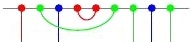 Figure 1
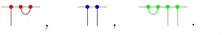 Figure 2
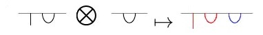 Figure 3
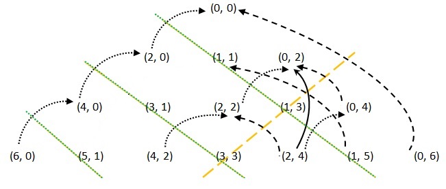 Figure 4