Structural Parameters for Scheduling with Assignment Restrictions
Klaus Jansen, Marten Maack, Roberto Solis-Oba

TL;DR
This paper investigates scheduling problems with assignment restrictions, analyzing how structural graph parameters like tree- and rankwidth influence computational complexity and approximation algorithms.
Contribution
It introduces three graphs based on assignment restrictions and studies their properties to identify cases with efficient algorithms, extending prior results.
Findings
Certain graph structures allow polynomial-time approximation schemes.
Tree- and rankwidth parameters are key to understanding problem complexity.
New algorithms are developed for specific graph classes.
Abstract
We consider scheduling on identical and unrelated parallel machines with job assignment restrictions. These problems are NP-hard and they do not admit polynomial time approximation algorithms with approximation ratios smaller than unless PNP. However, if we impose limitations on the set of machines that can process a job, the problem sometimes becomes easier in the sense that algorithms with approximation ratios better than exist. We introduce three graphs, based on the assignment restrictions and study the computational complexity of the scheduling problem with respect to structural properties of these graphs, in particular their tree- and rankwidth. We identify cases that admit polynomial time approximation schemes or FPT algorithms, generalizing and extending previous results in this area.
Click any figure to enlarge with its caption.
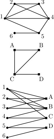 Figure 1
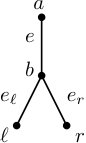 Figure 2
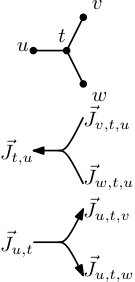 Figure 3
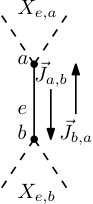 Figure 4
Peer Reviews
No public reviews on file for this paper yet. If you reviewed it on a platform where reviews are public (OpenReview, ICLR, NeurIPS, ICML), you can paste yours below so the community can read it here.
Videos
No videos yet. Explain this paper in a talk, walkthrough, or lecture? Add one.
Taxonomy
TopicsScheduling and Optimization Algorithms · Optimization and Search Problems · Distributed and Parallel Computing Systems
Structural Parameters for Scheduling with Assignment Restrictions111This work was partially supported by the DAAD (Deutscher Akademischer Austauschdienst) and by the German Research Foundation (DFG) project JA 612/15-1.
Klaus Jansen
University of Kiel, Kiel, Germany, {kj,mmaa}@informatik.uni-kiel.de
Marten Maack
University of Kiel, Kiel, Germany, {kj,mmaa}@informatik.uni-kiel.de
Roberto Solis-Oba
Western University, London, Canada, [email protected]
Abstract
We consider scheduling on identical and unrelated parallel machines with job assignment restrictions. These problems are NP-hard and they do not admit polynomial time approximation algorithms with approximation ratios smaller than unless P=NP. However, if we impose limitations on the set of machines that can process a job, the problem sometimes becomes easier in the sense that algorithms with approximation ratios better than exist. We introduce three graphs, based on the assignment restrictions and study the computational complexity of the scheduling problem with respect to structural properties of these graphs, in particular their tree- and rankwidth. We identify cases that admit polynomial time approximation schemes or FPT algorithms, generalizing and extending previous results in this area.
1 Introduction
We consider the problem of makespan minimization for scheduling on unrelated parallel machines. In this problem a set of jobs has to be assigned to a set of machines via a schedule . A job has a processing time for every machine and the goal is to minimize the makespan . In the three-field notation this problem is denoted by . On some machines a job might have a very high, or even infinite processing time, so it should never be processed on these machines. This amounts to assignment restrictions in which for every job there is a subset of machines on which it may be processed. An important special case of is given if the machines are identical in the sense that each job has the same processing time on all the machines on which it may be processed, i.e., . This problem is sometimes called restricted assignment and is denoted as in the three-field notation.
We study versions of and where the restrictions are in some sense well structured. In particular we consider three different graphs that are defined based on the job assignment restrictions and study how structural properties of these graphs affect the computational complexity of the corresponding scheduling problems. We briefly describe the graphs. In the primal graph the vertices are the jobs and two vertices are connected by an edge, iff there is a machine on which both of the jobs can be processed. In the dual graph, on the other hand, the machines are vertices and two of them are adjacent, iff there is a job that can be processed by both machines. Lastly we consider the incidence graph. This is a bipartite graph and both the jobs and machines are vertices. A job is adjacent to a machine , if . In Figure 1 an example of each graph is given. These graphs have also been studied in the context of constraint satisfaction (see e.g. [22] or [20]) and we adapted them for machine scheduling.
We consider the above scheduling problems in the contexts of parameterized and approximation algorithms. For an -approximation for a minimization problem computes a solution of value , where is the optimal value for a given instance . A family of algorithms consisting of -approximations for each with running times polynomial in the input length (and ) is called a (fully) polynomial time approximation scheme (F)PTAS. Let be some parameter defined for a given problem, and let be its value for instance . The problem is said to be fixed-parameter tractable (FPT) for , if there is an algorithm that given and solves in time , where is a constant, any computable function and the input length. This definition can easily be extended to multiple parameters.
Related work.
In 1990 Lenstra, Shmoys and Tardos [15] showed, in a seminal work, that there is a -approximation for and that the problem cannot be approximated with a ratio better than unless PNP. Both bounds also hold for and have not been substantially improved since that time. The case where the number of machines is constant is weakly NP-hard and there is an FPTAS for this case [11]. In 2012 Svensson [21] presented an interesting result for : A special case of the restricted assignment problem called graph balancing was studied by Ebenlendr et al. [6]. In this variant each job can be processed by at most machines and therefore an instance can be seen as a (multi-)graph where the machines are vertices and the jobs edges. They presented a approximation for this problem and also showed that the inapproximability result remains true. Lee et al. [14] studied the version of graph balancing where (in our notation) the dual graph is a tree and showed that there is an FPTAS for it. Moreover, the special case of graph balancing where the graph is simple has been considered. For this problem Asahiro et al. [2] presented among other things a pseudo-polynomial time algorithm for the case of graphs with bounded treewidth. For certain cases of with job assignment restrictions that are in some sense well-structured PTAS results are known. In particular for the path- and tree-hierarchical cases ([18] and [7]) in which the machines can be arranged in a path or tree and the jobs can only be processed on subpaths starting at the leftmost machine or at the root machine respectively, and the nested case ([17]), where , or holds for each pair of jobs .
The study of from the FPT perspective has started only recently. Mnich and Wiese [16] showed that is FPT for the pair of parameters and the number of distinct processing times. The problem is also FPT for the parameter pair and the number of machine types [12]. Two machines have the same type, if each job has the same processing time on them. Furthermore Szeider [23] showed that graph balancing on simple graphs with unary encoding of the processing times is not FPT for the parameter treewidth under usual complexity assumptions.
Results.
In this paper we present a graph theoretical viewpoint for the study of scheduling problems with job assignment restrictions that we believe to be of independent interest. Using this approach we identify structural properties for which the problems admit approximation schemes or FPT algorithms, generalizing and extending previous results in this area. The results are based on dynamic programming utilizing tree and branch decompositions of the respective graphs. For the approximation schemes the dynamic programs are combined with suitable rounding approaches.
Tree and branch decompositions are associated with certain structural width parameters. We consider two of them: treewidth and rankwidth. In the following we denote the treewidth of the primal, dual and incidence graph with , and , respectively. For the definitions of these concepts we refer to Section 2.
We now describe our results in more detail. Let be the set of jobs the machine can process. In the context of parameterized algorithms we show the following.
Theorem 1**.**
* is FPT for the parameter .*
Theorem 2**.**
* is FPT for the pair of parameters with and .*
Note that with constant remains NP-hard [6]. In the context of approximation we get:
Theorem 3**.**
* is weakly NP-hard, if or is constant and there is an FPTAS for both of these cases.*
The hardness is due to the hardness of scheduling on two identical parallel machines . The result for the dual graph is a generalization of the result in [14] and resolves cases that were marked as open in that paper. All results mentioned so far are discussed in Section 3. In the following section we consider the rankwidth:
Theorem 4**.**
There is a PTAS for instances of where the rankwidth of the incidence graph is bounded by a constant.
It can be shown that instances of with path- or tree-hierarchical or nested restrictions are special cases of the case when the incidence graph is a bicograph. Bicographs are known to have a rankwidth of at most (see [9]) and a suitable branch decomposition can be found very easily. Therefore we generalize and unify the known PTAS results for with structured job assignment restrictions.
2 Preliminaries
In the following will always denote an instance of or and most of the time we will assume that it is feasible. We call an instance feasible if for every job . A schedule is feasible if . For a subset of jobs and a subset of machines we denote the subinstance of induced by and with . Furthermore, for a set of schedules for we let , and if is the set of all schedules for . We will sometimes use . Note that there are no schedules for instances without machines. On the other hand, if is an instance without jobs, we consider the empty function a feasible schedule (with makespan [math]), and have therefore in that case.
Dynamic programs for .
We sketch two basic dynamic programs that will be needed as subprocedures in the following. The first one is based on iterating through the machines. Let for and , assuming . Then it is easy to see that . Using this recurrence relation a simple dynamic program can be formulated that computes the values . It holds that and as usual for dynamic programs an optimal schedule can be recovered via backtracking. The running time of such a program can be bounded by , yielding the following trivial result:
Remark 5**.**
* is FPT for the parameter .*
The second dynamic program is based on iterating through the jobs. Let . We call a load vector and say that a schedule fulfils , if . For let be the set of load vectors that are fulfilled by some schedule for the subinstance , assuming . Then can also be defined recursively as the set of vectors with and for , where and . Using this, a simple dynamic program can be formulated that computes for all . can be recovered from and a corresponding schedule can be found via backtracking. Let there be a bound for the number of distinct loads that can occur on each machine, i.e., for each . Then the running time can be bounded by , yielding:
Remark 6**.**
* is FPT for the pair of parameters and with .*
For this note that both and are bounds for the number of distinct loads that can occur on any machine. This dynamic program can also be used to get a simple FPTAS for for the case when the number of machines is constant. For this let be an upper bound of with . Such a bound can be found with the -approximation by Lenstra et al. [15]. Moreover let and . By rounding the processing time of every job up to the next integer multiple of we get an instance whose optimum makespan is at most bigger than . The dynamic program can easily be modified to only consider load vectors for , where all loads are bounded by . Therefore there can be at most distinct load values for any machine and an optimal schedule for can be found in time . The schedule can trivially be transformed into a schedule for the original instance without an increase in the makespan.
Tree decompostion and treewidth.
A tree decomposition of a graph is a pair , where is a tree, for each is a set of vertices of , called a bag, and the following three conditions hold:
- (i)
2. (ii)
3. (iii)
For every the set induces a connected subtree of .
The width of the decomposition is , and the treewidth of is the minimum width of all tree decompositions of . It is well known that forests are exactly the graphs with treewidth one, and that the treewidth of is at least as big as the biggest clique in minus . More precisely, for each set of vertices inducing a clique in , there is a node with (see e.g. [4]). For a given graph and a value it can be decided in FPT time (and linear in ) whether the treewidth of is at most and in the affirmative case a corresponding tree decomposition with nodes can be computed [3]. However, deciding whether a graph has a treewidth of at most , is NP-hard [1].
Branch decomposition and rankwidth.
It is easy to see that graphs with a small treewidth are sparse. Probably the most studied parameter for dense graphs is the cliquewidth . In this paper however we are going to consider a related parameter called the rankwidth . These two parameters are equivalent in the sense that [19]. Furthermore it is known that [5]. On the other hand cannot be bounded by any function in or , which can easily be seen by considering complete graphs.
A cut of is a partition of into two subsets. For let be the adjacency submatrix induced by and , i.e., if and otherwise for and . The cut rank of is the rank of over the field with two elements GF() and denoted by . A branch decomposition of is a pair , where is a tree with leaves whose internal nodes have all degree , and is a bijection from to the leafs of . For each there is an induced cut of : For the set contains exactly the nodes , where is a leaf that is in the same connected component of as , if is removed. Now the width of (with respect to ) is and the rankwidth of the decomposition is the maximum width over all edges of . The rankwidth of is the minimum rankwidth of all branch decompositions of . It is well known that the cliquewidth of a complete graph is equal to and this is also true for the rankwidth. For a given graph and fixed there is an algorithm that finds a branch decomposition of width in FPT-time (cubic in ), or reports correctly that none exists [10].
3 Treewidth Results
We start with some basic relationships between different restriction parameters for , especially the treewidths of the different graphs for a given instance. Similar relationships have been determined for the three graphs in the context of constraint satisfaction.
Remark 7**.**
* and .*
To see this note that the sets and are cliques in the primal and dual graphs, respectively.
Remark 8**.**
* and . On the other hand and .*
These properties were pointed out by Kalaitis and Vardi [13] in a different context. Note that this Remark together with Theorem 1 implies the results of Theorem 2 concerning the parameter . Furthermore, in the case of with only job and machines, or jobs and only machine the primal graph has treewidth [math] or and the dual or [math], respectively, while the incidence graph in both cases has treewidth .
Dynamic Programs
We show how a tree decomposition of width for any one of the three graphs can be used to design a dynamic program for the corresponding instance of . Selecting a node as the root of the decompostion, the dynamic program works in a bottom-up manner from the leaves to the root. We assume that the decomposition has the following simple form: For each leaf node the bag is empty and we fix one of these nodes as the root of . Furthermore each internal node has exactly two children and (left and right), and each node has one parent . We denote the descendants of with . A decomposition of this form can be generated from any other one without increasing the width and growing only linearly in size through the introduction of dummy nodes. The bag of a dummy node is either empty or identical to the one of its parent.
For each of the graphs and each node we define sets and of inactive jobs and machines along with sets and of active jobs and machines. The active jobs and machines in each case are defined based on the respective bag , and the inactive ones have the property that they were active for a descendant of but are not at . In addition there are nearly inactive jobs and machines , which are the jobs and machines that are deactivated when going from to its parent (for we assume them to be empty). The sets are defined so that certain conditions hold. The first two are that the (nearly) inactive jobs may only be processed on active or inactive machines, and the (nearly) inactive machines can only process active or inactive jobs:
[TABLE]
Where and for any sets and . Furthermore the (nearly) inactive jobs and machines of the children of an internal form a disjoint union of the inactive jobs and machines of , respectively:
[TABLE]
Where for any two sets emphasizes that the union is disjoint, i.e., . Now at each node of the decomposition the basic idea is to perform three steps:
- (i)
Combine the information from the children (for internal nodes). 2. (ii)
Consider the nearly inactive jobs and machines:
- •
Primal and incidence graph: Try all possible ways of scheduling active jobs on nearly inactive machines.
- •
Dual and incidence graph: Try all possible ways of scheduling nearly inactive jobs on active machines. 3. (iii)
Combine the information from the last two steps.
For the second step the dynamic programs described in Section 2 are used as subprocedures. We now consider each of the three graphs.
The primal graph.
In the primal graph all the vertices are jobs, and we define the active jobs of a tree node to be exactly the jobs that are included in the respective bag, i.e., . The inactive jobs are those that are not included in but are in a bag of some descendant of and the nearly inactive one are those that are active at but inactive at , i.e., and . Moreover the inactive machines are the ones on which some inactive job may be processed, and the (nearly in-)active machines are those that can process (nearly in-)active jobs and are not inactive, i.e., , and . For these definitions we get:
Lemma 9**.**
The conditions (1)-(4) hold, as well as:
[TABLE]
Proof.
[TABLE]
This yields (6) and (6) implies (1).
(2) and (5): Let and . We first consider the case that . Then there is a job with . If , we have and otherwise . Because of (T2) there is a node with . Since , we have . This together with (T3) gives . Now implies . Therefore we have . Next we consider he case that . In this case there is a job with and for each job we have . If we have and otherwise . Because of (T2) there is again a node with . Since , and we get using (T3). This also implies (5).
(3): All but follows directly from the definitions. Assuming there is a job we get because of (T3), yielding a contradiction.
(4): Because of (3) and the definitions we get , and for is clear by definition. Therefore it remains to show . We assume that there is a machine in this cut. Then there are jobs for with . We have and because of (T2) there is a node with . Because of and (T3) we have a contradiction. ∎
For and let . Let , and . We set and to be the sets of feasible schedules for the instances and respectively. We will consider and .
First note that , where is the root of . Moreover, for a leaf node there are neither jobs nor machines and holds. Hence let be a non-leaf node. We first consider how can be computed from the children of (Step (i)). Due to Property (iii) of the tree decomposition and (1) the jobs from are already active on at least one of the direct descendants of . Because of this and (4), may be split in two parts , where for . Let be the set of such pairs . From (3), (4) and (6) we get:
Lemma 10**.**
.
Proof.
Let be optimal. Since , we have for . Let . Because of (4) we have and obviously holds. Let . Because of (6) we have and (3) implies . This yields:
[TABLE]
Now let minimizing the righthand side of the equation and optimal. Then (3) and (4) imply that is in . Therefore we have . Since also equals the right hand side of the equation the claim follows. ∎
Consider the computation of (Step (iii)). We may split and into a set going to the nearly inactive and a set going to the inactive machines. We set to be the set of pairs with , and . Because of (3)-(5) we have:
Lemma 11**.**
.
Proof.
Let be optimal. Because of (5) we have . We set and . Then . Let and . Then and is a feasible schedule for . Because of (3) and (4), we have and:
[TABLE]
Now let minimizing the right hand side of the equation, and a feasible schedule for . Then (3) and (4) yield , and therefore . Since also equals the right hand side of the equation, the claim follows. ∎
Determining the values corresponds to Step (ii). Note that these values can be computed using the first dynamic program from Section 2 in time .
The dual graph.
For the dual graph the (in-)active jobs and machines are defined dually: The active machines for a tree node are the ones in the respective bag, the inactive machines are those that were active for some descendant but are not active for , and the nearly inactive machines are those that are active at but inactive at its parent, i.e., , and . Furthermore the inactive jobs are those that may be processed on some inactive machine and the (nearly in-)active ones are those that can be processed on some (nearly in-)active machine and are not inactive, i.e., , and . With these definitions we get analogously to Lemma 9:
Lemma 12**.**
The conditions (1)-(4) hold, as well as:
[TABLE]
∎
We will need some extra notation. Like we did in Section 2 we will consider load vectors , where is a set of machines. We say that a schedule fulfils , if for each . For any set of schedules for we denote the set of load vectors for that are fulfilled by at least one schedule from with . Furthermore we denote the set of all schedules for with , and for a subset of jobs , we write as a shortcut for . Let . We set and . Moreover, for and we set and to be those schedules that fulfil and respectively. We now consider and .
First note . Moreover, for a leaf node we have neither jobs nor machines and . Therefore . Hence let be a non-leaf node. Again, we first consider how can be computed from the children of . Because of (3) may be split into a left and a right part. For two machine sets let be a trasformation function for load vectors, where the -th entry of equals for and [math] otherwise. We set to be the set of pairs with , and for . Because of (1), (3) and (4), we have:
Lemma 13**.**
.
Proof.
Let be optimal. Because of (1) we have for . Let and the load vector that fulfils on . Then we have and . Because of (3) and (4) we have . Because of the objective function we have:
[TABLE]
Now let minimizing the right hand side of the equation and optimal. Then is in and equals the right hand side of the equation. Since furthermore the claim follows. ∎
Now we consider . We may split into the load due to inactive and that due to nearly inactive jobs. Note that the nearly inactive jobs can only be processed by active machines (7). We set to be the set of pairs with , and . Now (3), (4) and (7) yield:
Lemma 14**.**
.
Proof.
Let be optimal. Then (7) implies . We set and . Furthermore let be the load vector fulfilled by and the one fulfilled by on . Then is a feasible schedule for fulfilling , and . Furthermore (3) yields . We get:
[TABLE]
Now let minimizing the right hand side of the equation, and a feasible schedule for fulfilling . Then and therefore . Since also equals the right hand side of the equation, the claim follows. ∎
The set can be computed using the second dynamic program described in Section 2 in time if is again a bound on the number of distinct loads that can occur on each machine.
The incidence graph.
For the incidence graph we combine the ideas that we used for the two other graphs. The situation is slightly more complicated because we have to handle the jobs and machines simultaneously. All the job sets are defined like in the primal, and all the machine sets like in the dual graph case. With these definitions the conditions (1)-(4) follow almost directly from the definitions together with (T2) and (T3). The proofs for the recurrence relations in this paragraph have the same structure as the proofs for the other recurrence relations and no new ideas are needed. Therefore they are omitted.
Let , and . We set to be the set of feasible schedules for that schedule the jobs from on inactive machines, i.e., for each . Moreover, is the set of schedules for that schedule the jobs from on (nearly) inactive machines . The sets of schedules that in addition fulfil a load vector or are denoted by and . We consider and .
First note . For a leaf note there are neither jobs nor machines and therefore . Hence let be a non-leaf node. Like before, we first consider . Both and may be split into a left and a right part and we set like before. Moreover, for we define to be the set of pairs with for . Due to (1)-(4) we have:
Lemma 15**.**
. ∎
Next we consider . The set again may be split into a part going to the inactive and a part going to the nearly inactive machines, while the nearly inactive jobs have to be split into a part going to the inactive and a part going to the active machines (note that in this case (7) does not hold). Therefore, we set to be the set of pairs with , , and . The splitting of is more complicated as well, because in this case all of the active machines may receive load from the nearly inactive jobs, and the nearly inactive machines may additionally receive load from the active but not nearly inactive jobs ((5) does not hold). Therefore we set to be the set of triplets with , , and . Due to (3) and (4) we have:
Lemma 16**.**
. ∎
Note that the sets and can be computed in time using the second dynamic program described in Section 2, if is again a bound on the number of distinct loads that can occur on each machine.
Results.
Using above arguments, we can design dynamic programs with running time in the primal case and in the dual and incidence graph cases. Optimal schedules can be found via backtracking proving the Theorems 1 and 2. Theorem 3 follows by the combination of the dynamic programs and a rounding scheme similar to that in Section 2.
4 Rankwidth Results
First we want to argue that there is not much to be gained when considering primal or dual graphs with bounded rankwidth. For this consider any instance of . By adding a job with processing time that can be processed on every machine, and a machine that can only process this new job, we get a modified instance . Any schedule for one of the instances can trivially be transformed into a schedule for the other without an increase in the makespan. However, while the rankwidth of the primal or dual graph of could have been arbitrarily high, the rankwidth of the primal and dual graph of are both equal to one, because these graphs are complete.
We study the case when the rankwidth of the incidence graph is bounded by a constant . Moreover we assume that also the number of distinct job sizes is bounded by a constant, which we can do because of the following result. Let be some class of instances of , which is invariant with respect to changing the processing times of jobs and the introduction of copies of jobs.
Lemma 17** (Rounding Lemma).**
If there is a PTAS for instances from , for which the number of distinct processing times is bounded by a constant, then there is also a PTAS for any instance from .
Proof.
Let , and an upper bound of with . Such a bound can be found in polynomial time for example with the -approximation by Lenstra et al. [15]. Moreover let . We call jobs big, if and otherwise small. Next, we construct a modified instance . This instance has the same machine set and for each big job a job with the same restrictions and processing time is included in the job set. This yields . For each small job in we introduce many jobs with the same restrictions as , and with processing time .
Note that has a has at most many distinct processing times and that . Moreover the size of is polynomial in the size of .
Given an optimal solution of , consider the solution of we get by scheduling both the big and the small jobs in the same way as there analogues in . The big jobs on a machine can cause an increase of the processing time of at most factor , while for each small job of there may be an increase of at most . Therefore we get:
[TABLE]
Now given a PTAS for instances of for which the number of distinct processing times is bounded by a constant, we can compute a schedule for with in polynomial time. We use to construct a schedule for for . In this schedule the big jobs are assigned in the same way as there analogous in . For the small jobs we need some additional consideration. Let and be the set of small jobs in and respectively. Moreover, for let be the set of small jobs that were inserted in due to . The assignment of in can be seen as a fractional assignment of . We find a rounding for this fractional assignment of the small jobs. For each machine and small job let . Furthermore let be the summed up processing time that machine receives in the schedule from small jobs, i.e., . Then is a solution of the following linear program:
[TABLE]
Using the rounding approach by Lenstra et al. [15], we can transform this in polynomial time into an integral solution fulfilling the constraint (9) and instead of (10) the modified constraint:
[TABLE]
We set to assign the small jobs according to . Since we get and together with the above considerations:
[TABLE]
∎
While all of the used techniques are well known they have—to the best of our knowledge—not been used in the indicated way up to now.
It can be easily seen that the class of instances of , for which the rankwidth of the incidence graph is bounded by a constant , is invariant with respect to changing the processing time of jobs and the introduction of copies of jobs.
Dynamic Program
We present a dynamic program to solve using a branch decomposition with rankwidth for the incidence graph. First we give some intuition on why a bounded rankwidth is useful.
For any Graph and , we say that have the same connection type with respect to if . If is clear from the context we say that and have the same connection type. Now, let be some edge of the branch decomposition and the respective cut of , i.e., for is the set of vertices of that are in the same connected component as when the edge is removed. Then induces a partition of both the jobs and machines by and for .
Remark 18**.**
Let with . The number of distinct connection types of with respect to is bounded by .
We actually use that the number of distinct connection types of the jobs is bounded.
In the rest of this section we first show how the branch decomposition can be used in a straightforward way to solve (with exponential running time). The basic idea for this is that each edge of the decomposition corresponds to a partition of the job and machine sets and an optimal solution may be found by trying all possible ways of moving jobs between partitions. At the machine-leafs all arriving jobs have to be processed, with no jobs going out, and at the job-leafs all jobs have to be send away, with no jobs coming in. From this the procedure can work up to some root edge. Next we argue that it is sufficient to consider only certain locally defined classes of job sets. The crucial part here is that the number of these classes can be polynomially bounded, because the number of distinct sizes and connection types of jobs are constant.
Job sets.
Let again be some edge of the tree and the corresponding cut of . We fix a schedule and make some basic observations. There is a set of jobs that assigns to machines from . We will use the intuition that is sent through from to (see also Figure 2). The node may be an inner node or a leaf. Moreover, if is a leaf, may be a job or a machine . In the first case sends no jobs to , and to . In the second case no jobs are sent to and the jobs send to should be feasible on . Now any set that is sent through an edge and arrives at an internal node, will be split into two parts: one going forth through the second and one through the third edge. And looking at it the other way around: Any set that is sent by a schedule through an edge coming from an inner node, is put together from two parts, one coming from the second and one coming from the third edge.
We formalize this notion. Let be an internal node of , with neighbours . Then for each pair of neighbours of there are job sets , such that:
[TABLE]
See also Figure 3. It is rather easy to see that sets that are feasible at the leafs and fulfil the conditions (11) uniquely define a feasible schedule.
Using these observations, we now discuss how (the value of) an optimal schedule can be found by considering different job sets that may be sent through the edges. For this we use an intuition of up and down, with above and below. Let and be some candidate sets to be sent up and down respectively through . We set for with , i.e., the subinstances of induced by , if and are send up or down respectively. Note that the instance is split into the two subinstances. Moreover let be the set of pairs . Then:
[TABLE]
We now consider the computation of for the two cases when is an internal node or a leaf. If is a leaf, it may correspond to a job or a machine, i.e., or . In the first case we get if or , and otherwise. In the second case is empty since there are no jobs at . We get if and otherwise.
Now let be an internal node that is connected to two lower nodes and via edges and (Figure 4). We say that and are on the left, while and are on the right. Recursively we assume that for any and we know and respectively. We want to identify the set of tuples that for fixed may occur in a schedule, i.e., fulfil condition (11) for all edges from . For it is clear which part is coming from the left and which from the right and we set and accordingly, such that . The other four sets in which the job sets going up and down could be split can all be tried. More precisely, for each with , and the tuple is in and the set is defined by such tuples. We get:
[TABLE]
Using these considerations can be solved by choosing a root edge that is incident to a leaf corresponding to a job and designing a dynamic program working from leaf edges to the root edge using (13). Now (12) for together with the considerations for leaf nodes yield . The running time of such an algorithm is exponential in the input length.
Classes of Jobs.
Let . There are some cases in which and are in some sense similar and it holds that . This is the case if there is a bijection such that and have the same connection type with respect to and for each . By this, an equivalence relation can be defined, and analogously a relation . Now the observation (12) can be reformulated in terms of equivalence classes:
Lemma 19**.**
.∎
Note that in this equation equivalence classes and are considered belonging to the relations and respectively. and are arbitrary representatives of these classes. We will now develop a sensible representation for the equivalence classes.
We drop the notion of up and down for the following considerations, i.e., is just one of two nodes of some edge . We assume some ordering of the different processing times, with denoting the -th processing time for . Any set of jobs induces a vector where is the number of jobs in that have the -th processing time, i.e., . We set . Let be the number of connection types of jobs from with respect to . Note that due to Remark 18 we get . Again assuming some ordering, for let be the size vector induced by the -th connection type of with respect to and the machines from the respective jobs may be processed on. Moreover let . Now the equivalence classes of can naturally be represented and characterized by vectors .
Remark 20**.**
For each and there are at most different vectors .
We now study the splitting behaviour of job classes at inner nodes. Consider a set that is sent through an edge and then forth through an incident edge . Then there are vectors and representing in the context of and respectively. However, some other set represented by will also be represented by , that is translates uniquely into . We formalize this notion by the definition of a translation function . For each there is a unique with , i.e., the -th connection type of translates into the -th connection type of . Let be given by . Now for each we set , with and more precisely . With this we can formulate an analogue of (11). For a fix schedule let be the representative of the set of jobs that sends from to . Now let be an inner node with neighbours . For neighbours of , the set considered in the last paragraph now has a representative in the contexts of and . Fixing the first one , the second one can be obtained via a transformation function, yielding:
[TABLE]
From now on we will use the up and down notion like before ( with above and below). Let and be candidate job classes to be send up and down . Considering Lemma 19 we set to be the minimum value where is represented by and by .
For the case when is a leaf not much changes. If is a job , the class of has only one element and is represented by . Therefore we get that for and , and otherwise. If is a machine , we have and there are only two possible connection types for jobs from , because jobs can be processed on or not, i.e., . In any case we get .
Now let be an inner node again with lower neighbours and to which it is connected via edges and . We may assume that we know the values and for candidate job classes to go up or down the left or right edge respectively. We want to identify the set of quadruples that are compatible with and , i.e., that fulfil (14). For this let with , with , and with , such that . By setting , , and we get such a tuple and the set is defined by such tuples.
Lemma 21**.**
.
Proof.
If the righthand side equals , it is easy to see that the equation holds, and we will therefore assume . For given and let be any set represented by and an optimal one represented by , i.e., minimizing . Let be an optimal schedule for . Furthermore let , , and be the sets that sends up or down through or respectively, and let , , and their classes. Than induces schedules and for and . We get:
[TABLE]
Now let minimizing the right hand side of of the considered equation with corresponding splitting vectors . Moreover let and be optimal sets represented by and respectively. Splitting , and corresponding to the splitting of their job classes we can obtain sets , and that are represented by , and respectively and fulfil (11). We have now and . Let and be respective optimal schedules. Than is a schedule for and equals the right hand side of the considered equation. Since was chosen optimal with an optimal class representative we have furthermore . This yields:
[TABLE]
Moreover we get that is optimal as well. ∎
Results.
With these considerations a dynamic program for can be defined. This can be done in a way such that its running time is in , proving Theorem 4 together with the Rounding Lemma and the considerations of Section 2.
Bi-cographs
We show that the path- and tree-hierarchical and nested cases are all special cases of the case that the incidence graph is a bi-cograph. Bi-cographs were introduced as a bipartite analogue of cographs [8].
Definition 22**.**
For a bipartite graph the bi-complement of is the graph . A graph is called bi-cograph, iff it is bipartite and can be reduced to isolated vertices by recursively bi-complementing its connected bipartite subgraphs.
It is known [9] that their cliquewidth and therefore also their rankwidth is bounded by . Furthermore by recursively bi-complementing the connected bipartite subgraphs, a certain decomposition of a given bi-cograph can be found in linear time that is similar to cotrees of cographs [8]. This decomposition can easily be turned into a branch decomposition, for which in the application studied here the number of connection types of jobs for every edge of the decomposition and is bounded by .
Lemma 23**.**
Let be an instance of with path- or tree-hierarchical or nested restrictions. Then the incidence graph of is a bi-cograph.
Proof.
We first consider the case that has tree hierarchical restrictions. Let be a corresponding rooted tree with . Then there is at least one machine (the root of ) that can process all jobs. After bi-complementing the connected bipartite subgraphs of the incidence graph this machine is isolated. This can be repeated: After bi-complementing two more times the nearest descendants of the root in that cannot process all jobs will be isolated. Iterating this, at some point all machines and therefore also all jobs will be isolated.
Now let be an instance with nested restrictions. Note that the jobs with maximal (with respect to ) are all in different connected components of the incidence graph and connected to all machines in their component. Hence they are isolated after bi-complementing the first time. If we bi-complement a second time and remove these jobs we get a new instance with nested restrictions and less jobs. By iterating this argument the claim follows. ∎
Acknowledgements.
The Rounding Lemma in the presented form was formulated by Lars Rohwedder and Kevin Prohn as part of a student project.
The reference list from the paper itself. Each links out to its DOI / PubMed record.
- 1[1] Stefan Arnborg, Derek G Corneil, and Andrzej Proskurowski. Complexity of finding embeddings in ak-tree. SIAM Journal on Algebraic Discrete Methods , 8(2):277–284, 1987.
- 2[2] Yuichi Asahiro, Eiji Miyano, and Hirotaka Ono. Graph classes and the complexity of the graph orientation minimizing the maximum weighted outdegree. Discrete Applied Mathematics , 159(7):498–508, 2011.
- 3[3] Hans L Bodlaender. A linear-time algorithm for finding tree-decompositions of small treewidth. SIAM Journal on computing , 25(6):1305–1317, 1996.
- 4[4] Hans L Bodlaender. A partial k-arboretum of graphs with bounded treewidth. Theoretical computer science , 209(1):1–45, 1998.
- 5[5] Derek G Corneil and Udi Rotics. On the relationship between clique-width and treewidth. SIAM Journal on Computing , 34(4):825–847, 2005.
- 6[6] Tomáš Ebenlendr, Marek Krčál, and Jiří Sgall. Graph balancing: A special case of scheduling unrelated parallel machines. Algorithmica , 68(1):62–80, 2014.
- 7[7] Leah Epstein and Asaf Levin. Scheduling with processing set restrictions: Ptas results for several variants. International Journal of Production Economics , 133(2):586–595, 2011.
- 8[8] Vassilis Giakoumakis and Jean-Marie Vanherpe. Bi-complement reducible graphs. Advances in Applied Mathematics , 18(4):389–402, 1997.