This paper investigates a higher-degree generalization of the S-lemma related to Hilbert's theorem on ternary quartics, demonstrating its limitations through geometric and algebraic analysis within quadratic modules.
Contribution
It introduces new tools to analyze the non-existence of a higher-degree S-lemma generalization, linking geometric and algebraic perspectives.
Findings
01
Higher-degree S-lemma generalization is not possible without extra conditions.
02
Established a connection between geometric and algebraic reasons in quadratic modules.
03
Extended tools by Netzer to analyze positivity and stability in polynomial modules.
Abstract
In this work we will investigate a certain generalization of the so called S-lemma in higher degrees. The importance of this generalization is, that it is closely related to Hilbert's 1888 theorem about tenary quartics. In fact, if such a generalization exits, then one can state a Hilbert-like theorem, where positivity is only demanded on some semi-algebraic set. We will show that such a generalization is not possible, at least not without additional conditions. To prove this, we will use and generalize certain tools developed by Netzer ([Ne]). These new tools will allow us to conclude that this generalization of the S-lemma is not possible because of geometric reasons. Furthermore, we are able to establish a link between geometric reasons and algebraic reasons. This will be accomplished within the framework of quadratic modules.
No public reviews on file for this paper yet. If you reviewed it on a platform where reviews are public (OpenReview, ICLR, NeurIPS, ICML), you can paste yours below so the community can read it here.
Videos
No videos yet. Explain this paper in a talk, walkthrough, or lecture? Add one.
Taxonomy
TopicsAdvanced Optimization Algorithms Research · Polynomial and algebraic computation · Commutative Algebra and Its Applications
Full text
Higher degree S-lemma and the stability of quadratic modules
Philipp Jukic
Abstract
In this work we will investigate a certain generalization of the so called S-lemma in higher degrees.
The importance of this generalization is, that it is closely related to Hilbert’s 1888 theorem about tenary quartics. In fact, if such a generalization exits, then one can state a Hilbert-like theorem, where positivity is only demanded on some semi-algebraic set.
We will show that such a generalization is not possible, at least not without additional conditions. To prove this, we will use and generalize certain tools developed in [Ne]. In fact, these new tools will allow us to conclude that this generalization of the S-lemma is not possible because of geometric reasons. Furthermore, we are able to establish a link between geometric reasons and algebraic reasons. This will be accomplished within the framework of quadratic modules.
First of all, let us talk about the motivation of this article. In 1888 Hilbert showed in his work [Hi] that a ternary quartic f, that is a 4-form in three variables, can be written as a sum of three squares of quadratic forms if and only if f is non-negative on R3. The question is: Can we find a Hilbert-like theorem in a more general setting? What does a more general setting mean in this context? Instead of considering non-negative ternary quartics, we consider a ternary quartic that needs to be non-negative on a semi-algebraic set S⊆R3. Furthermore, the semi-algebraic set S should also satisfy the following two conditions: First, there exists a quadratic form g in three variables such that S=S(g):={x∈R3:g(x)≥0}. Second, the set S has a non-empty interior.
Of course, if S=R3 then f can, in general, not be written as a sum of three squares of quadratic forms. In this case we need a sort of a correcting term. This correcting term should also satisfy some conditions. First, we demand that this term is of the form −tg, where t is a non-negative quadratic form. Second, f−tg should be a non-negative ternary quartic.
Thus a generalization of Hilbert’s theorem could look like the following:
Let g be a quadratic form such that there exists a point x′∈R3 with g(x′)>0.
A ternary quartic f is non-negative on the set S(g) if and only if there exists a non-negative quadratic form t such that f−tg can be written as a sum of three squares of quadratic forms.
The interpretation of this statement is simple. If g is non-negative, then this statement is equal to Hilbert’s statement. If g is not non-negative, then −tg measures ’how far away’ f is from being a sum of three squares of quadratic forms.
Let us illustrate this statement by considering the two polynomials g=x12−x22 and f=x14−x24. It is easy to see that S(g) has a non-empty interior and that f is non-negative on S(g). Furthermore, we have f−2x22g=x14−2x12x22+x24=(x12−x22)2. Thus f−2x22g is a sum of three squares of quadratic forms: One quadratic form is given by x12−x22, the other two are [math].
We are looking to clarify the following question: Can such a generalization of Hilbert’s theorem be made? It turns out that this question is closely related to the so called S-lemma resp. to a certain generalization of the S-lemma.
Hence the first Chapter is all about the introduction and the proof of the S-lemma. The machinery presented in this chapter relies heavily on the work of [PT] and [Bar].
The results in the first chapter are all well known. Therefore there is nothing new in this part of the article.
In this chapter and throughout the whole article no fancy knowledge will be required. One should be familiar with basic linear algebra, convex geometry, and real algebraic geometry.
In the second Chapter we will formulate a generalization of the S-lemma. For the sake of simplicity we will refer to the generalization as the S4-conjecture.
The importance of this S4-conjecture is the following: If the conjecture is true, then the generalization of Hilbert’s theorem is possible. If it is not true, then such a generalization is impossible. However, it turns out that it is impossible because we can find a counterexample for the S4-conjecture.
Although we can find a counterexample, we will still refer to this mentioned generalization as the S4-conjecture.
Next, we do some geometric investigations and finally generalize the counterexample to higher degrees. In the third and last chapter we use and generalize the machinery developed in [Ne] to further investigate the counterexample.
It turns out that the tools presented in [Ne] are quite suitable in analyzing the S4-conjecture.
In fact, by using these new methods we will see that the conjecture fails because of geometric reasons.
Since [Ne] connects geometric properties and algebraic properties, we will see that there is an interesting link between the S4-conjecture and the stability of quadratic modules.
Finally, this article will be concluded by presenting some new questions that should serve as a motivation for further studies.
We will use the following notation throughout this article:
•
R, C, Z, N,N0: The real, complex, integer, natural numbers and the natural numbers with [math].
•
Rn, Cn, Zn: The 0≤n dimensional vector spaces Rn resp. Cn and the free Z-module Zn.
•
⟨⋅,⋅⟩: The standard scalar product in Rn.
•
K[x1,…,xn]: The polynomial ring over a field K in n≥1 variables. Polynomial variables will always be denoted by upright letters x,y,\upbeta,\uplambda etc.
•
K[x1,…,xn]d: The set of all polynomials f∈K[x1,…,xn] with deg(f)≤d.
•
A polynomial f∈R[x1,…,xn] is called non-negative if ∀x∈Rn:f(x)≥0. Negative, positive and non-positive polynomials are defined in the same manner.
•
The homogenization of a polynomial f∈K[x1,…,xn] will be denoted by f. The dehomogenization of a homogeneous polynomial g with g~.
•
An, Pn: The n-dimensional affine space and the n-dimensional projective space.
•
V(f1,…,fs): For polynomials f1,…,fs∈K[x1,…,xn] the set V(f1,…,fs) is defined to be the set of all solutions x∈Kn (K denotes the algebraic closure of K) of the polynomial equalities f1(x)=0,…,fs(x)=0. If K=R then we will fix C as the algebraic closure of R. If f1,…,fs are homogeneous, then we can interpret V(f1,…,fs) as the set of all solutions in the projective space Pn.
•
Let V be a variety defined over a field K and L∣K an algebraic extension of K. The L-rational points of V are denoted by V(L).
•
S(f1,…,fs): The basic closed semi-algebraic set
[TABLE]
defined by the polynomials f1,…,fs∈R[x1,…,xn].
•
GLn, On: The general linear group over R and its orthogonal subgroup over R.
•
Let X be a topological space and A a subset. The interior of A is denoted with int(A) and the closure with A.
Chapter 1 The S-lemma
In this chapter we will formulate and prove the so called S-lemma. Before doing this, however, it shall be noted that the S-lemma has many variations in the literature. While all versions are in fact equivalent, we will use a version that is closer to real algebraic geometry. Thus the original statement of the S-lemma made by Yakubovich, that can be found in the work of Polik and Terlaky [PT], will not be used. In the sense of real algebraic geometry the S-lemma is formulated in the following way:
Theorem 0.1**.**
S-lemma:
Let f,g be polynomials in R[x1,…,xn]2. If there exists a point x′∈Rn with g(x′)>0, then the following statements are equivalent:
(a)
The inclusion S(g)⊆S(f) holds.
2. (b)
There exists a non-negative real number t such that f(x)−tg(x)≥0 for all x∈Rn
The aim of this chapter is to provide a proof for Theorem 0.1. Simultaneously, it should serve as an introduction in what is to come later. Before we are ready to prove Theorem 0.1, we need some preparatory results, which will be bundled together in the following section.
1 Preliminaries
First of all, it is worth mentioning that one could prove Theorem 0.1 directly, without any notable machinery. One such proof can be found in [PT, pp. 376-378]. The disadvantage is, however, that it needs quite a lot of computations. As already pointed out, we will use a different approach. For the proof of theorem 0.1 we will need the following definitions, lemmas, and propositions:
Definition 1.1**.**
Let f=∑i=1n∑j=1naijxixj be a quadratic form in R[x1,…,xn], where all coefficients aij of f lie in R.
The matrix that corresponds to f is defined to be
the symmetric matrix Af=(21(aij+aji))1≤i≤n,1≤j≤n.
If f is an arbitrary form of degree d≥0 in R[x1,…,xn], then f is said to be positive semi-definite resp. positive definite if ∀x∈Rn:f(x)≥0 resp. ∀x∈Rn\{0}:f(x)>0.
Remark 1.2**.**
A quadratic form f is positive (semi-) definite if and only if the corresponding matrix Af is positive (semi-) definite.
In the following we will assume that the coefficients of a quadratic form in R[x1,…,xn] lie in R.
Definition 1.3**.**
Let Pd,n be the set of all forms of even degree d>0 in R[x1,…,xn]. With Pd,n+ we denote the subset of Pd,n that consist of all positive semi-definite forms in Pd,n.
Definition 1.4**.**
Let V be finite dimensional R-vector space. A (convex) cone C⊆V is a subset of V that satisfies the following two conditions:
•
The set C is not empty.
•
For any real number λ≥0 and any element g∈C we have λg∈C.
We say that a cone C⊆V is pointed, if the identity C∩−C={0} holds.
Remark 1.5**.**
One can easily see that P2,n is a finite dimensional R-vector space. To be more precise, there is a vector-space isomorphism P_{2,n}\xrightarrow{\,\smash{\raisebox{-2.15277pt}{\scriptstyle\sim}}\,}\mathbb{R}^{\frac{n(n+1)}{2}}. For f,g∈P2,n the dot product on P2,n is defined by ⟨f,g⟩=tr(AfAg), which is just the pullback of the dot product in R2n(n+1). Thus P2,n is an euclidean space. The same is also true for Pd,n, where d≥0.
Finally, it should be noted that this vector space P2,n has a more or less surprising upcoming in algebraic geometry: See [Sha I, Example 3, p. 44] about determinantal varieties.
Definition 1.6**.**
Let V be a finite dimensional real vector space and C⊆V a convex subset. A convex subset F of C is called a face of C if the following statement holds:
Suppose u and v are two points in C. If there exists a λ∈(0,1) such that λu+(1−λ)v∈F, then u and v lie already in F.
A face F of C is called proper if ∅⫋F⫋C holds. If there is a point u∈C such that {u} is a face of C, then the point u is called an extremal point. With ex(C) we will denote the set of all extremal points of C.
Definition 1.7**.**
Let V be a finite dimensional real vector space and C⊆V a convex subset. Let H be a hyper plane given by H={x∈V:ℓ(x)=0}, where ℓ:V→R is a linear form. Set H+={x∈V:ℓ(x)≥0} and H−={x∈V:ℓ(x)≤0}. A face F of C is called exposed if there exists a linear form ℓ:V→R such that C is contained in H+ or H− and F=C∩H.
Definition 1.8**.**
Let V be a finite dimensional real vector space and S an arbitrary subset of V. The affine hull aff(S) of S is defined by
[TABLE]
Definition 1.9**.**
Let V be a finite dimensional real vector space. The dimension of a convex set C⊆V is defined to be the dimension of its affine hull. In short dim(C)=dim(aff(C)).
Definition 1.10**.**
Let V be a finite dimensional real vector space and C a convex subset of V. Let Bε(x) denote the open ball in x with radius ε>0. The relative interior relint(C) of C in V is defined by
[TABLE]
Lemma 1.11**.**
(a): For every x∈Rn\{0} the symmetric n×n-matrix xxT matrix is positive semi-definite of rank 1.
(b): Let A be a positive semi-definite matrix. The rank of A is the smallest natural number r such that A can be written as A=∑i=1rxixiT for some x1,…,xr∈Rn.
Proof: (a): Trivial.
(b): First of all, note that statement (b) is independent with respect to transformations STAS, where S∈On. Indeed, set D=STAS and assume that A=∑i=1rxixiT, where r is minimal. Then we have D=ST∑i=1rxixiTS=∑i=1rSTxixiTS=∑i=1rSTxi(STxi)T.
It is clear that r is also the minimal length of the sum for D: Otherwise, A could be written as a sum of smaller length, which would be a contradiction. Choose S∈On such that D is a diagonal matrix. The diagonal of D consists of the eigenvalues of A, which are all non-negative. Thus it is easy to see that D can be written as a sum ∑i=1rxixiT for some x1,…,xn∈Rn and r=rk(A). It remains to verify that r is minimal. But this follows from rk(∑i=1rxixiT)≤rrk(xixiT)=r. \boxempty
Proposition 1.12**.**
Let d≥0 be an even number.
(a)
The set Pd,n+ is a closed cone in Pd,n.
2. (b)
The cone Pd,n+ is pointed.
3. (c)
Let L⊆Rn be a subspace and FL:={f∈P2,n+:∀x∈L:f(x)=0}. The set FL is an exposed face with dim(FL)=2r(r+1) and r=n−dim(L). If f∈P2,n+ and L=ker(Af), then f is in relint(FL).
Proof: (a): We will show that P:=Pd,n\Pd,n+ is open. Take an element f∈P.
Since f∈P, there exists a point x∈Rn such that f(x)<0. Consider the evaluation homomorphism evx:Pd,n→R,p↦p(x). Furthermore, Pd,n is, as already stated in Remark 1.5, an euclidean space. Thus evx is continuous. Let U⊆R be an open neighborhood of f(x) such that all elements of U are negative real numbers.
The set U′=evx−1(U) is an open neighborhood of f that satisfies U′⊆P. Thus we proved that P is open resp. that Pd,n+ is closed. The second assertion that Pd,n+ is a cone is trivial.
(b): Trivial.
(c):
In the following we will just omit the trivial parts of the proof.111Pay attention to statements that begin with ’It is easy to see’.
Let us begin with the easiest part, verifying that dim(FL)=2r(r+1), where r=n−dim(L). This can be done by proving aff(FL)≅R2r(r+1).
Let L⊥ be the orthogonal complement of L in Rn. Without loss of generality we can identify L with Rn−r and L⊥ with Rr.
Consider the cone P2,r+. It is easy to see that FL can be identified with P2,r+. Furthermore, P2,r+ has a non-empty interior. A well known result in convex geometry states that a cone with non-empty interior is full. This means that aff(P2,r+)=P2,r. Thus aff(P2,r+)≅R2r(r+1). Identifying aff(FL) with aff(P2,r+) proves the assertion.
Next, we show that FL is an exposed face. A quadratic form h1∈P2,n−r+ and a quadratic form h2∈P2,r+ give rise to a quadratic form h∈P2,n+ in an obvious manner. In fact, the corresponding matrix Ah of h is given by A_{h}=\left(\begin{array}[]{cc}A_{h_{1}}&0\\
0&A_{h_{2}}\end{array}\right). Fix h1=x12+⋯+xn−r2 and define \tilde{A}_{h_{1}}=\left(\begin{array}[]{cc}A_{h_{1}}&0\\
0&0\end{array}\right), \tilde{A}_{h_{2}}=\left(\begin{array}[]{cc}0&0\\
0&A_{h_{2}}\end{array}\right). Then we can identify FL with {h∈P2,n+:∃h2∈P2,r+:Ah=A~h2}. It is easy to see that FL consists of all quadratic forms h∈P2,n+ that satisfy tr(AhA~h1)=0. Thus it is convenient to consider the linear form ℓ:P2,n→R,p↦tr(ApA~h1) and the hyper plane H={p∈P2,n:ℓ(p)=0}. So far, we know that FL=P2,n+∩H.
Finally, we just have to deal with the inclusion P2,n+⊆H+. Let h=∑i,jaijxixj be a quadratic form in P2,n+. Since h is non-negative, the coefficients aii must be non-negative for all i=1,…,n. Thus the diagonal of Ah consists of non-negative real numbers. This implies ℓ(h)≥0. Altogether we proved that FL is an exposed face.
Let us deal with the last statement in (c). Suppose f∈P2,n+ and L=ker(Af). As before set r=n−dim(L). Again we identify FL with P2,r+ and interpret f as a quadratic form in P2,r+.
Then f does only vanish at the origin in Rr.
Hence f lies in the interior of the cone P2,r+ resp. in relint(FL), which proves the assertion. \boxempty
Lemma 1.13**.**
Let C⊂Rn be a non-empty closed convex set which does not contain any straight line. Then ex(C) is a non-empty set.
Because the next result is very important, it will be proven, although there exists a suitable reference.
Proposition 1.14**.**
Let L be an affine subspace of P2,n such that S=L∩P2,n+ is not empty. Suppose the inequality codimP2,n(L)<2(r+2)(r+1) holds for some r∈N0. Then there exists a quadratic form f∈S such that the rank of Af is bounded by r.
Proof[Bar, Proposition 13.1, p. 83]: According to Proposition 1.12 the cone P2,n+ is pointed and closed. This means that there is no way that the cone P2,n+ contains a straight line. If P2,n+ does not contain such a line so does not the subset S of P2,n+. By using Lemma 1.13 we get ex(S)=∅. Choose an arbitrary f∈S and let Af be its corresponding matrix of rank m. Consider W=ker(Af) and the exposed face FW (Proposition 1.12). We want to show that f is an element of the set relint(L∩FW). Since f is an element of relint(FW) and relint(L), it is enough to verify the inclusion relint(FW)∩relint(L)⊂relint(L∩FW).
Take a point g∈relint(FW)∩relint(L). There exist ε1,ε2>0 such that Bε1(g)∩aff(FW)⊂FW and Bε2(g)∩aff(L)⊂L. By setting ε=min{ε1,ε2} we get Bε(g)∩aff(L)∩aff(FW)⊂L∩FW. Since aff(L∩FW)⊂aff(L)∩aff(FW), we have Bε(g)∩aff(L∩FW)⊂L∩FW which implies the assertion.
We know that f lies in both sets, relint(L∩FW) and ex(L∩FW). This can only work if dim(L∩FW)=0 holds: Suppose dim(L∩FW)>0. For every ε>0 we can find two different points δ1,δ2∈Bε(f) such that δ1,δ2=f and δ1,δ2,f∈aff(L∩FW). Choose ε>0 such that Bε(f)∩aff(L∩FW)⊂L∩FW holds. Now, f is some point on the line segment that connects the two points δ1 and δ2. But both points lie in L∩FW. This contradicts the fact that f is an extremal point of L∩FW.
Since dim(L∩FW)=0, we get dim(L)+dim(FW)=dim(L+FW)≤dim(P2,n). This and Proposition 1.12 imply 2m(m+1)=dim(FW)≤dim(P2,n)−dim(L)=codimP2,n(L)<2(r+1)(r+2) and thus m<r+1. \boxempty
Corollary 1.15**.**
Let f1,f2∈P2,n be two quadratic forms. The two equations f1(x)=α1 and f2(x)=α2 have a simultaneous solution x∈Rn if and only if there exists a quadratic form q∈P2,n+ such that tr(Af1Aq)=α1 and tr(Af2Aq)=α2.
Proof[Bar, Corollary 13.2, p. 84]: ⇒: Choose x∈Rn such that f1(x)=α1 and f2(x)=α2. Define X=xxT. Then tr(AfiX)=tr(AfixxT)=xTAfix=fi(x)=αi holds for i=1,2.
⇐: The map ℓi:P2,n→R,p↦tr(AfiAp) is obviously a vector space homomorphism for i=1,2.
It is easy to see that ℓi−1(αi)=ker(ℓi)+q holds for i=1,2. Hence dim(ℓi−1(αi))=dim(P2,n)−1 for i=1,2.
This implies codimP2,n(L)<3=2(1+1)(2+1), where L=ℓ1−1(α1)∩ℓ2−1(α2). According to Proposition 1.14 we can find a quadratic form h in L∩P2,n+ such that tr(AfiAh)=αi and rk(Ah)≤1 for i=1,2. Now, Lemma 1.11 tells us that there exists a point x∈Rn with Ah=xxT. Substituting Ah through xxT in tr(AfiAh) results in fi(x)=αi for i=1,2. \boxempty
Corollary 1.16**.**
Consider the quadratic forms f1,f2∈P2,n and the map φ:Rn→R2,x↦(f1(x),f2(x))T. Then the set M=φ(Rn) is a convex subset of R2.
Proof[Bar, Corollary 13.3, p. 84]: Consider the map
[TABLE]
Since ψ is linear and P2,n+ is a cone (Proposition 1.12), the image of P2,n+ under ψ is a cone. Finally, Corollary 1.15 implies the equality ψ(P2,n+)=M. \boxempty
Proposition 1.17**.**
Let A and B be two non-empty convex subsets of Rn such that A∩B=∅. Then there exists a linear form ℓ:Rn→R such that ℓ(x)≤ℓ(y) for all x∈A and y∈B.
Proof: See [Bar, Proposition 1.2, p. 106]. \boxempty
2 Proof of the S-lemma
Before actually proving theorem 0.1 we will consider a special case, from which the Theorem 0.1 will easily follow.
Proposition 2.1**.**
Homogeneous S-lemma:
Let f,g be quadratic forms in
R[x1,…,xn]. If there exists a point x′∈Rn with g(x′)>0, then following statements are equivalent:
(a)
The inclusion S(g)⊆S(f) holds.
2. (b)
There exists a non-negative real number t≥0 such that f(x)−tg(x)≥0 for all x∈Rn
Proof[PT, Proposition 2.3, p. 377]: (b)⇒(a): This implication is quite trivial: Suppose we could find a non-negative real number t such that f(x)−tg(x)≥0 holds for all x∈Rn and a point y∈Rn with g(y)≥0 and f(y)<0. It is clear that f(y)−tg(y) would be negative, contradicting f(x)−tg(x)≥0 for all x∈Rn.
(a)⇒(b): According to Corollary 1.16 the set M={(f(x),g(x)):x∈Rn} is a convex subset of R2. Define C={(u1,u2):u1<0,u2≥0}. Because S(g)⊆S(f) holds, the intersection between M and the convex set C is empty. According to Proposition 1.17 there exists a linear form ℓ:R2→R such that ℓ(x)≤ℓ(y) for all x∈M and y∈C. Since 0∈M and 0∈C, we have ℓ(x)≤0≤ℓ(y) for all x∈M and y∈C.
Choose α1,α2∈R such that ℓ=α1x1+α2x2.
Consider the two statements
[TABLE]
If we take the point (−1,0)∈C and evaluate ℓ at (−1,0), we get ℓ(−1,0)=−α1≥0. Thus α1 must be a non-positive real number.
For an arbitrary ε>0 the point (−ε,1) lies in C. Evaluating ℓ at the point (−ε,1) leads to ℓ(−ε,−1)=−α1ε+α2≥0. If α2=0 then α2 must be positive. Otherwise, we could choose ε>0 so small that the inequality −α1ε+α2<0 would hold.
We know that there exists a point x′∈Rn such that g(x′)>0. From the inequality α1f(x′)+α2g(x′)≤0 we conclude that α1 cannot vanish. Set α=α1α2.
Without loss generality we can assume that α=0. Otherwise, f would be non-negative and therefore we could set t=0.
Since α<0, we have the inequality αα1f(x)+αα2g(x)=α2(f(x)+αg(x))≥0 for all x∈Rn. Hence f+αg is a non-negative polynomial. Set t=−α and the assertion follows. \boxempty
Proof of theorem 0.1: (b)⇒(a): This implication is trivial.
(a)⇒(b): Without loss of generality we can assume that x′=0.
Set x=(x1,…,xn).
Let
[TABLE]
be the decompositions of f and g with respect to the standard grading in R[x],
where f1 resp. g1 denotes the component of f resp. g that has degree 2, f2 resp. g2 denotes the component of f resp. g that has degree 1 and finally, cf resp. cg denotes the constant component. Let f,g∈R[x,y] be given by:
[TABLE]
In fact, we just need to prove that f and g satisfy the condition (a) in Proposition 2.1: Since then, there would exist a non-negative real number t such that f(x,y)−tg(x,y)≥0 for all (x,y)∈Rn+1 and the assertion would follow from the dehomogenization of f(x,y)−tg(x,y).
Suppose we could find a point (x,y)∈Rn+1 with y=0 such that
[TABLE]
Then we would get a contradiction, since the two identities
[TABLE]
hold.
Suppose we could find a point (x,0)∈Rn+1 with
[TABLE]
This two inequalities imply that f1(x)<0 and g1(x)≥0. Consider f(\uplambdax)=\uplambda2f1(x)+\uplambdaf2(x)+cf as a polynomial in the new variable \uplambda. Since f1(x)<0, we get that λ2f1(x)+λf2(x)+cf converges to −∞ as ∣λ∣ converges to ∞.
Acknowledging that cg>0, g1(x)≥0 and treating g(\uplambdax)=\uplambda2g1(x)+\uplambdag2(x)+cg as a polynomial in \uplambda, leads us to the following distinctions
•
g(λx)→∞ for λ→∞ if g1(x)>0
•
g(λx)→∞ for λ→sign(g2(x))∞ if g1(x)=0 and g2(x)=0.
This proves that no matter what, we can always find a suitable λ∈R such that f(λx)<0 and g(λx)≥0 are satisfied, which clearly contradicts our assumption. \boxempty
Chapter 2 Higher degree S-lemma
1 Counterexample
Let us revisit Proposition 2.1. The question here is, if there is a generalization of the mentioned proposition in higher degrees. To be more precise, can we give up the restriction that the degree of the two homogeneous polynomials in Proposition 2.1 is bounded by 2? The answer is no, as the following simple example illustrates it.
Example 1.1**.**
Consider g=x12−x22 and f=x12(x12−x22). Then there is no non-negative real number t such that f(x)−tg(x)≥0 holds for all x∈R2. It is easy to check that g and f satisfy the prerequisites and the condition (a) of Proposition 2.1. Suppose we could find a non-negative real number t such that f(x)−tg(x)≥0 holds for all x∈R2. Let (kn)n⊂R be a sequence such that kn→0 for n→∞. The inequality f(kn,0)−tg(kn,0)≥0 implies f(kn,0)≥tg(kn,0) for all n∈N. But this is not true. Choose a natural number N∈N such that kN2<t. Then tg(kN,0) would be greater than f(kN,0), which would contradict
our assumption.
{window}
[3, r, ,]
Remark 1.2**.**
Since we cannot generalize Proposition 2.1 to higher degrees (Example 1.1), the method we used to prove Proposition 2.1 should also fail in higher degrees. The interesting question is, where does it fail? In case of Lemma 1.1 it turns out that the set M={(f(x),g(x)):x∈R2} is not a convex subset of R2 anymore. We reprise that g=x12−x22 and f=x12(x12−x22).
Consider the half-line H={λ(−1,1):λ∈R≥0}.
Since S(g)⊆S(f) holds, the intersection M∩H can only consist of one point and this point is the origin (0,0).
On the other hand, we can find two points (x1,x2),(y1,y2)∈M such that x1>0, x2>0, y1<0, y2<0 and the line segment L connecting the points (x1,x2), (y1,y2) does not go through the origin. This means L intersects H in some other point than the origin.
But this intersection point cannot be in M. Thus M is not convex.
{window}
[3, r, ,]
Example 1.3**.**
Consider the two homogeneous polynomials q=x13x2−x12x22 and p=x14−x1x23.
We want to show that M={(p(x),q(x)):x∈R2} is not convex, giving an example where M fails to be convex even if both homogeneous polynomials have the same degree. Set H={(0,x2):x2<0}.
There are points (x1,x2),(y1,y2)∈M with x1<0,x2<0,y1>0,y2<0 such that the segment line L, connecting both points, doesn’t go through the origin. So the intersection point of L and H is not in M. Thus M is not convex.
2 Formulating a higher degree S-lemma
In the past section we have seen that there is no way to increase the degree in the homogeneous S-lemma (Proposition 2.1) and keep all other statement as they are.
There are two ways one can proceed. One way would be to left the conditions (a) and (b) in the homogeneous S-lemma unchanged, and find some additional statements that might be plugged in into the homogeneous S-lemma such that the S-lemma remains true. Results in this sense can be found in [ZS].
But there is another way. Instead of keeping the statements (a) and (b) as they are, we could simply modify the condition (b) by giving up that t should be a non-negative real number. We demand that t should be a non-negative homogeneous polynomial. The advantage is that we do not need to make up some new statements. The disadvantage, however, is that we have less information about t. This philosophy motivates to formulate
Conjecture 2.1**.**
S4-Conjecture: Let f be a tenary quartic, that is a 4-form in R[x1,x2,x3], and let g be a quadratic form in R[x1,x2,x3]. Suppose there exists a point x′∈R3 such that g(x′)>0. Then the following statements are equivalent:
(a)
The inclusion S(g)⊆S(f) holds.
2. (b)
There exists a non-negative homogeneous polynomial t∈R[x1,x2,x3]2 such that f(x)−t(x)g(x)≥0 for all x∈R3.
The statement 2.1 is originally a question posted in Mathoverflow and was answered by the author. See [MathOver].
Remark 2.2**.**
The homogeneous polynomial t in the S4-conjecture is either a quadratic form or the zero-polynomial, which can be interpreted as a homogeneous polynomial of negative-infinite degree. The case t=0 can only occur if f is a non-negative form. If f is not a non-negative form, then t must be of degree 2. This becomes clear if we take a point x∈/S(f).
Then we get f(λx)−t(λx)g(λx)=λ4f(x)−λ2t(x)g(x)≥0 for all λ≥0 (). Note that if t is not of degree 2, then it must be a constant.
But no matter what sign the constant t has, we will always get λ4f(x)−λ2t(x)g(x)→−∞ for λ→∞, which contradicts ().
Since g is a quadratic form, we can take a look at the signature of g. If the S4-conjecture fails, then the next obvious question is: Is there a counterexample for all non-trivial signatures −1,0 and 1. Note that if the signature of g is −2 resp. 2, then g is non-positive resp. non-negative. But it is obvious how to deal with the S4-conjecture if g is non-positive or non-negative.
3 S4-conjecture in two variables
In this section we are going to prove the S4-conjecture in just two variables aka.
Theorem 3.1**.**
S4-conjecture in 2-variables: Let f be a 4-form in R[x1,x2] and let g be a quadratic form in R[x1,x2]. Suppose there exists a point x′∈R2 such that g(x′)>0. Then the following statements are equivalent:
(a)
The inclusion S(g)⊆S(f) holds.
2. (b)
There exists a non-negative homogeneous polynomial t∈R[x1,x2]2 such that f(x)−t(x)g(x)≥0 for all x∈R2.
Remark 3.2**.**
Theorem 3.1 is not true, without the condition that there exists a point x′∈R2 such that g(x′)>0! Consider for example the polynomials g=−x12 and f=x14+x13x2+x1x23. Obviously g is a non-positive quadratic form and the equation g(x1,x2)=0 holds if and only if x1=0. But for x1=0 we have f(0,x2)=0, which implies S(g)⊆S(f). Take a homogeneous polynomial t=a1x12+a2x22+a3x1x2, where a1,a2,a3∈R. Then f(x1,1)−t(x1,1)g(x1,1)=x14+x13+x1+a1x14+a2x12+a3x13. But no matter what the coefficients a1,a2,a3 are, the polynomial f(x1,1)−t(x1,1)g(x1,1) has a sign change at the origin. Thus the implication (a)⇒(b) in Theorem 3.1 would be false.
Lemma 3.3**.**
Let p and q be polynomials in R[x] such that deg(p)=4, deg(q)=2 and S(q)⊆S(p). Suppose that there exists a point x′∈R with q(x′)>0. Then there exists a non-negative polynomial t∈R[x] of degree at most 2 such that p(x)−t(x)q(x)≥0 for all x∈R.
Proof: Without loss of generality we can assume that neither p nor q are non-negative polynomials. Otherwise we could just take t=0.
For the sake of simplicity and oversight we will devide the proof in several meaningful cases:
Case I: The polynomial p has a real double root y∈R: In this situation p is divided by s=(x−y)2∈R[x]. Set h=sp∈R[x]. It is clear that h is a polynomial of degree 2 and that the inclusion S(q)⊆S(h) holds:
The only situation in which S(q)⊆S(h) might fail is the one, where y is an isolated point of S(q). But this would imply that s∣q, which means that q is either a non-negative or a non-positive polynomial. Obviously non of these two cases can occur.
According to the S-lemma (Theorem 0.1) there is a non-negative real number t′≥0 such that h(x)−t′q(x)≥0 for all x∈R. This implies that the inequality 0≤s(x)(h(x)−t′q(x))=p(x)−t′s(x)q(x) holds for all x∈R. Set t=t′s and the assertion follows.
Case II: The polynomial p has a complex root c∈C\R: If c is a complex root of p, then p is divided by the polynomial s=(x−c)(x−c)∈R[x]. Since s has only complex roots, we conclude that s is nowhere changing its sign. It is easy to see that limx→∞s(x)=∞. Thus s is non-negative. By defining h=sp and repeating the procedure in case I, we get the desired result.
Case III: The polynomial p has four distinct real roots x1<x2<x3<x4: Here we
have two possibilities how q may actually look like. If there exists a point c∈[x1,x2] such that p(c)<0, then q=α(x−x~1)(x−x~4) for α>0 and x~1≤x1, x~4≥x4. If there exists a point c∈[x1,x2] such that p(c)>0, then q=α(x−x~1)(x−x~4) for α<0 and x~1≥x1, x~4≤x4.
Consider the first possibility. Define h=α(x−x1)(x−x4) and s1=h′(x1)p′(x1), s4=h′(x4)p′(x4). Note that h′ does not vanish at x1 resp. x4. Thus s1 and s4 are well defined positive real numbers.
Let v∈R[x] be a positive polynomial of degree 2 such that v(x1)=s1 and v(x4)=s4. For example, consider the polynomial v=a(x−x1)2+s1 with a=(x4−x1)2s4−s1 if s1≤s4 resp. the polynomial v=a(x−x4)2+s4 with a=(x1−x4)2s1−s4 if s1>s4.
The polynomial w=p−vh has two double roots, namely one double root at x1 and the other at x4. This proves that w is either non-negative or non-positive. Since w(x3)>0, the polynomial w is indeed non-negative.
It is easy to see that the inclusion S(q)⊆S(h) holds. According to the S-lemma there exists a real non-negative number t′ such that h(x)−t′q(x)≥0 holds for all x∈R. This implies −h(x)≤−t′q(x) for all x∈R and therefore w(x)≤p(x)−t′v(x)q(x). Since w is non-negative, we are done. The second possibility is considered nearly analogous:
Without loss of generality we can assume that x1≤x~1, x2≥x~4 and h=α(x−x1)(x−x2).
As before we define s1=h′(x1)p′(x1) resp. s2=h′(x2)p′(x2). Let v be a positive polynomial of degree 2 such that v(x1)=s1 and v(x2)=s2 are satisfied. The polynomial w=p−vh has two double roots at x1 and x2. Since w(x4)>0, we see that w is non-negative. As before we can deduce from S(q)⊆S(h) that there exists a positive real number t′ with h(x)−t′q(x)≥0 for all x∈R, implying that w(x)≤p(x)−t′v(x)q(x) for all x∈R. Set t=t′v and we are done. It is clear that there are no cases left that can occur. Thus the lemma is proven. \boxempty
Lemma 3.4**.**
Let q∈R[x1,…,xn] be a quadratic form such that there exists a point x′∈Rn with q(x′)>0. For every point x∈S(q) and for every ε>0 the intersection between Bε(x) and int(S(q)) is non-empty.
Proof: By using an appropriate change of coordinates we can rewrite q as q=a1x12+⋯+anxn2, where a1,…,an∈R.
Define I={i∈{1,…,n}:ai>0}. Note that I=∅ because of q(x′)>0. Take a point x∈Rn with q(x)≥0.
Choose an index j∈I, a real positive number ε>0 and consider q(x1,…,xj+ε,…,xn) if xj≥0 resp. q(x1,…,xj−ε,…,xn) if xj<0. It is clear that q(x1,…,xj+ε,…,xn) resp. q(x1,…,xj−ε,…,xn) is positive.
This means that the point y={(x1,…,xj+ε,…,xn),ifxj≥0(x1,…,xj−ε,…,xn),ifxj<0 is lying in both, the interior of S(q) and the ball Bε(x). In other words, the assertion is proven. \boxempty
Lemma 3.5**.**
Let p∈R[x1,…,xn] be a polynomial of even degree m∈N0 and q∈R[x1,…,xn] a polynomial of degree 2. Suppose further that there is a point x′∈Rn such that q(x′)>0. Let p,q∈R[x1,…,xn+1] denote their homogenizations. If S(q)⊆S(p) then S(q)⊆S(p).
Proof:
We have to show that S(q(x,0))⊆S(p(x,0)) holds. Without loss of generality we can assume that S(q(x,0))=∅.
Note that q(x′)>0 implies q(x′,1)>0. Thus we can use Lemma 3.4.
Let c be an arbitrary point in S(q(x,0)). The task is to verify c∈S(p(x,0)). Lemma 3.4 tells us that Bε(c)∩int(S(q))=∅ for ε>0. For every ε>0 we can find a point yε∈Bε(c)∩int(S(q)) such that the n+1-th component of yε does not vanish. We have q(yε,1,…,yε,n+1)=yε,n+121q(yε,n+1yε,1,…,yε,n+1yε,n,1), where q(yε,n+1yε,1,…,yε,n+1yε,n,1)>0. Therefore p(yε,n+1yε,1,…,yε,n+1yε,n,1)≥0. Since m is even, we get p(yε,1,…,yε,n+1)=yε,n+1m1p(yε,n+1yε,1,…,yε,n+1yε,n,1)≥0.
This implies that dist(c,S(p))<ε. By making ε>0 arbitrary small and using the fact that S(p) is a closed set, we conclude that c∈S(p). \boxempty
Proof of Theorem 3.1 aka. S4-conjecture in 2 variables: Without loss of generality we can restrict ourselves to the case where f and g are both not non-negative.
(b)⇒(a): Trivial.
(a)⇒(b): Since we are talking about quadratic forms, and g is a quadratic form, it helps to take a look at its diagonal-form. Let us take a matrix A∈O2 and consider the induced map ψ:R[x1,x2]→R[x1,x2],p↦p∘A. We can choose A in such a way that ψ(g) is in diagonal form. Applying ψ on f and g does not mess up the prerequisites of Theorem 3.1. Thus we can assume that g is already in diagonal from. Since g is neither non-negative nor non-positive, two real numbers a11,a22=0 with sgn(a11)=sgn(a22) can be found such that g=a11x12+a22x22. Furthermore, we can demand that a11>0 and a22<0 because otherwise we could apply the coordinate transformation R2→R2,(x1,x2)↦(x2,x1). The proof is devided into two cases:
Case I: degx1(f) and degx2(f)<4: First of all, we show that the monomial x13x2 cannot appear in f, while the monomials x12x22 and x1x23 must appear in f. Suppose the monomial x13x2 would appear in f. Consider the polynomial f(x1,1)∈R[x1]. Since S(g)⊆S(f), we get the conditions limx1→∞f(x1,1)=∞ and limx1→−∞f(x1,1)=∞. But the leading term of f(x1,1) is of the form αx13 for α=0.
Thus f1(x1,1) cannot fulfill the two conditions and therefore we get a contradiction. On the other side, we cannot exclude the monomial x1x23. In case of the monomial x2x13 we exploited that the set S(g(x1,1)) is symmetric and unbounded. This is not the case when we consider S(g(1,x2)). Instead we can state that since f is non-negative on the set S(g), the polynomial f cannot consist of just one monomial x1x23 or x12x22 alone. So, we can rewrite f as f=γx12x22+βx1x23 with γ>0 and β∈R\{0}.
Define s=−21ba22x24+21ba11x12x22+βx1x23 and t=21bx22 where a11b=γ>0. A simple computation shows f=tg+s. We are done, if we can show that s is a non-negative polynomial. Since s is divided by x22, it is sufficient to prove that s′=x22s=−21ba22x22+βx1x2+21ba11x12 is non-negative. The discriminant of s′ is given by disc(s′)=(β2+a22a11b2)x12. Then we have the equivalence disc(s′)≤0 for all x1∈R⇔β2+a22a11b2≤0.
It is sufficient to show that β2+a22a11b2≤0.
To prove this, take a point y∈∂S(g) such that y1,y2>0. Furthermore we assume that β<0. Now y∈∂S(g) implies y1=y2a11a22 and thus f(y)=(γa11a22+βa11a22)y24≥0. This is only possible if γa11a22+βa11a22≥0. The inequality γa11a22+βa11a22≥0 is equivalent to γa11a22≥∣β∣. By substituting γ through a11b, we get ∣a11a22∣b≥∣β∣ and finally β2+a11a22b2≤0, because a11a22<0.
If β>0 then we simply consider another point y∈∂S(q) with y1>0, y2<0, and repeat the arguments above.
Case II: degx1(f)=4 or degx2(f)=4: We are only considering the case degx1(f)=4. Let f~∈R[x1] be the dehomogenization of the polynomial f in the variable x2.
In the same manner, let g~∈R[x1] be the dehomogenization of g. It is easy to see that f~ and g~ fulfill the prerequisites of Lemma 3.3. Thus there exists a non-negative polynomial t~∈R[x1] with deg(t~)≤2 such that f~(x1)−t~(x1)g~(x1)≥0 for all x1∈R.
If f~(x1)−t~(x1)g~(x1)=0 holds for all x1∈R, then the assertion follows immediately.
Otherwise, Lemma 3.5 tells us that S(f~−t~g~)=R and S(t~)=R imply S(f~−t~g~)=R2 and S(t)=R2, where t={t~ifdeg(t~)=2x22t~ifdeg(t~)=0.
If deg(t~)=2 then we get that f−tg=x24(f~−t~g~), f−tg=x22(f~−t~g~) or
f−tg=f~−t~g~. This follows directly from the fact that f~−t~g~ is of even degree and that deg(f)=deg(tg).
If deg(t~)=0 then it is easy to see that f−tg=f~−t~g~. Thus f−tg is non-negative. \boxempty
4 The S4-conjecture: A counterexample
It turns out that the S4-conjecture stated in 2.1 is wrong. First of all, we are going to give a ’lucky’ counterexample and afterwards, that means in the next chapter, we will investigate why the S4-conjecture cannot work.
Example 4.1**.**
A counterexample for 2.1: Consider the polynomials f=x13x3+x13x2+x22x32 and g=x1x3+x2x3+x1x2. One can show that the inclusion S(g)⊆S(f) holds: For example, type in
But there is no non-negative homogeneous polynomial t∈R[x1,x2,x3] of degree at most 2 such that f(y)−t(y)g(y)≥0 for all y∈R3: Suppose we could find such a polynomial t=a1x12+a2x22+a3x1x2+a4x1x3+a5x2x3+a6x32, where a1,…,a6∈R. A simple computation shows that f−tg=x13x2−a1x13x2−a3x12x22−a2x1x23+x13x3−a1x13x3−a1x12x2x3−a3x12x2x3−a4x12x2x3−a2x1x22x3−a3x1x22x3−a5x1x22x3−a2x23x3−a4x12x32−a4x1x2x32−a5x1x2x32−a6x1x2x32+x22x32−a5x22x32−a6x1x33−a6x2x33.
Thus f(x1,0,1)−t(x1,0,1)g(x1,0,1)=x13−a1x13−a4x12−a6x1. We know that f−tg is a non-negative polynomial. This is only possible if a1=1, a6=0, and a4≤0. Since t is non-negative and a6=0, the two coefficients a4, a5 must also vanish. The leading term of f(0,x2,1)−t(0,x2,1)g(0,x2,1) is −a2x23, and therefore a2=0. Now only a3 is not determined. But it is easy to see that a3 must also vanish. Thus f−tg reduces to f−tg=−x12x2x3+x22x32, which is obviously not non-negative.
Remark 4.2**.**
Under an appropriate linear change of coordinates, we can rewrite g as g=x12−21x22−21x32. Thus under this new coordinates S(g) is a double cone and every slice with a plane, parallel to the x2,x3-plane, is compact. Fix c>0 and consider S:=S(c2−21x22−21x32), which is a compact subset of R2. A simple computation shows that f(c,x2,x3)>0 for all x2,x3∈S. Using the Positivstellensatz of Schmüdgen, we see that f(c,x2,x3)∈T(g(c,x2,x3)), where T(g(c,x2,x3)) denotes the preordering generated by g(c,x2,x3). This, however, is not true for f and g, i.e f∈/T(g). See Lemma 5.1 and Remark 5.2.
5 Geometric analysis
In this section we are going to take a closer look at the counterexample. In particular we are interested in the geometric properties of V1=V(f) and V2=V(g) and what they have to do with the counterexample. In this section we will fix f=x13x3+x13x2+x22x32 and g=x1x3+x2x3+x1x2.
Lemma 5.1**.**
Let f and g be as in Example 6. Then there is no non-negative homogeneous polynomial t∈R[x1,x2,x3] of even degree n such that f(y)−t(y)g(y)≥0 for all y∈R3.
Proof:
Without loss of generality we can assume that n>2.
Let t be a non-negative homogeneous polynomial in R[x1,x2,x3] of even degree n>2. We are going to show that f(x1,x2,1)−t(x1,x2,1)g(x1,x2,1) is not a non-negative polynomial in R[x1,x2], which is a stronger statement than that in the lemma. Because f(x1,x2,0)=x13x2 is not non-negative, we can assume that t(x1,x2,0)=0. Thus we have deg(t(x1,x2,0))=n.
Write t(x1,x2,1)=∑α∈N2,∣α∣≤ncαxα and define I={α∈N2:∣α∣=n,cα=0}. Note that I is not empty, since deg(t(x1,x2,0))=n.
Without loss of generality we can assume that there is an element α∈I such that α2>0. Otherwise, we could simply interchange the variables x1 and x2.
Let α′ be the uniquely determined element of I that satisfies α2′>α2 for all α∈I\{α′}. There exists a real number β>0 such that cα′βα2′+∑α∈I\{α′}cαβα2=0: Indeed, ∑α∈Icα\upbetaα2 is a polynomial in R[\upbeta] of degree α2′>0 and therefore does not vanish.
In fact, ∑α∈Icαβα2 is the leading coefficient and ∑α∈Icαβα2x1α1+α2=∑α∈Icαβα2x1n the leading term of the polynomial t(x1,βx1,1).
So, the real positive number β is needed to make sure that this leading term does not vanish.
Because t(x1,βx2,1) is non-negative, the coefficient ∑α∈Icαβα2 is positive. The leading term of tg is (∑α∈Icαβα2+1)x1n+2 with a positive coefficient ∑α∈Icαβα2+1. This implies that the leading term of f−tg is −(∑α∈Icαβα2+1)x1n+2. Therefore we get
[TABLE]
which proves the lemma. \boxempty
Remark 5.2**.**
Lemma 5.1 combined with the Counterexample 4.1 proves that f∈/T(g). Suppose we could find sums of squares σ1 and σ2 in R[x1,x2,x3] such that f=σ1+σ2g. Then we have f~=σ~1+σ~2g~, where we dehomogenize with respect to x3. Without loss of generality we can assume that deg(σ~2)≥2. We distinguish between two cases:
•
We have deg(σ~2g~)=deg(f~)=4: Under this condition, we have f−σ~2g=x3n(f~−σ~2g~), where n≤4 is a even number.
By using Lemma 3.5 we see that f~−σ~2g~ is non-negative.
Thus f−σ~2g is non-negative. Since σ~2 is a non-negative polynomial of degree 2, we get a contradiction.
•
We have deg(σ~2g~)>deg(f~)=4: In this case we proceed as in Lemma 5.1: Choose a real positive number β such that the leading monomial of f(x1,βx1,1)−σ2(x1,βx1,1)g(x1,βx1,1) is −Lβx12, where L denotes the leading monomial of σ2(x1,βx1,1). Since σ2(x1,βx1,1) is a sum of squares in R[x1], the polynomial L is a sum of squares and therefore Lβx12 is non-negative.
Thus
[TABLE]
which contradicts our assumption.
Lemma 5.3**.**
The two R-varieties V(g) and V(f) are both geometrically irreducible. Furthermore, the set H={(0,x2,0):x2∈R} is the set of all R-rational singularities of V(g) and V(f).
Proof: First, V(f) resp. V(g) is irreducible if and only if V(f~) resp. V(g~) is irreducible, where f~=x13+x13x2+x22 and g~=x1+x2+x1x2. This statement is a well known fact.
Consider the polynomial g~ as an element of the ring C[x1][x2]. Furthermore, g~ is a primitive polynomial. According to [Bo, Satz 2, p. 68] we know that g~ is irreducible in C[x1][x2] if the image of g~ in (C[x1]/x1C[x1])[x2] is irreducible, which is easy to verify.
Hence V(g~) is an irreducible C-variety.
Let us consider f~ as an element of the polynomial ring C[x1][x2].
The polynomial f~ cannot be divided by any irreducible polynomial in C[x1]: Indeed, C[x1][x2]/x1C[x1][x2]≅(C[x1]/x1C[x1])[x2] and the image of f~ in (C[x1]/x1C[x1])[x2] is not a unit.
Suppose an irreducible factor h of f~ has the same degree in x2 as f~. Then h must coincide with f~: If there would exist another irreducible factor v, then v must lie in C[x1]. But this would be a contradiction, since v∤f~. It is impossible that f~ factors into more than one component in C[x1][x2]:
Suppose we could write f~=h1h2, where h1,h2∈C[x1][x2] are polynomials of degree 1 in x2. The polynomials h1 and h2 can be written as h1=x2−v1 and h2=x2−v2, where v1,v2∈C[x1]. Then f~=x22−x2v2−x2v1+v1v2. Therefore v1v2=x13 and −x2(v1+v2)=x2x13, which is utterly impossible.
Hence V(f~) is an irreducible C-variety.
It remains to verify the statement about the singularities. Consider a point x∈V(f~) such that ∇f~(x)=0. Then we have ∇f(x′)=0 for x′=(x,1). On the other hand, suppose there is a point x′∈V1 with x3′=0 such that ∇f(x′)=0. Then the point x=(x3′x1′,x3′x2′) will satisfy ∇f~(x)=0.
This shows that the singular points x′∈V1 with x3′=0 ’come from’ the singular points of V(f~). Thus it suffices to show that V(f~) has only one R-rational singularity at the origin and that all other R-rational singularities of V1 are in H.
The equation \nabla\tilde{f}(x)=\left(\begin{array}[]{c}3x_{1}^{2}+3x_{1}^{2}x_{2}\\
x_{1}^{3}+2x_{2}\end{array}\right)=0 has only one real solution x=(0,0) in V(f~), proving the first assertion of the last statement.
Finally, consider the equation \nabla f(x_{1},x_{2},0)=\left(\begin{array}[]{c}3x_{1}^{2}x_{2}\\
x_{1}^{3}\\
x_{1}^{3}\end{array}\right)=0, where the set of all solutions in R3 is exactly H. Note that H is a subset of V(f)(R) and V(g)(R). The same argumentation applied to g gives the same result. Thus the lemma is proven. \boxempty
Remark 5.4**.**
A standard theorem in algebraic geometry states that a irreducible variety V over C is connected with respect to the norm topology. For a proof see [Sha II, Theorem 1, p. 126]. In 5.3 we proved that V2=V(g) is irreducible. Thus V2⊆C2 is a connected set. But it is easy to see that V2(R) is not connected. This implies that [Sha II, Theorem 1, p. 126] is not true if we just consider the R-rational points.
Lemma 5.5**.**
Let (qn)n be a convergent sequence of quadratic forms in R[x1,…,xn] and (pn)n a convergent sequence of forms in R[x1,…,xn] of degree d such that S(qn)⊆S(pn) for every n∈N. If q and p are the limits of the sequences (qn)n and (pn)n, then S(q) is a subset of S(p) if q=0.
Proof:
First of all we are going to prove the assertion under the assumption that int(S(q))=∅.
Under an appropriate change of coordinates we can assume that q=a1x12+⋯+anxn2, where a1,…,an∈R.
For every point y∈S(q) there exists a sequence (yn)n⊂int(S(q)) such that limn→∞yn=y.
Since int(S(q)) is not empty, we can handle this statement with Lemma 3.4.
Consider a point x lying in the interior of S(q). Then there exists a number N∈N such that qn(x)>0 for all n≥N, implying that limn→∞qn(x)≥0. Since S(qn) is a subset of S(pn), we get limn→∞pn(x)≥0 resp. x∈S(p).
If x lies in ∂S(q), then there exists a sequence (xn)⊂int(S(q)) such that limn→∞xn=x. But we showed above that this sequence also lies in S(p). Thus x lies in S(p), since S(p) is closed.
Finally, the case int(S(q))=∅ must be considered. This is only possible if the coefficients of q=a1x12+⋯+anxn2 are all non-positive and at least one of them is negative. If all coefficients are negative, then we are done, since any form in R[x1,…,xn] is non-negative at the origin. Therefore we can assume that not all coefficients are negative. Thus the set I′={i∈{1,…,n}:ai=0} is not empty. Set H=∏i∈/I′R×∏i∈I′{0}, H′=∏i∈I′R×∏i∈/I′{0} and consider q′=q∣H, p′=p∣H. Then we have S(q′)={0} by assumption and therefore S(q′)⊆S(p′). Since S(q)=S(q′)∪H′, we have to make sure that p′′=p∣H′ is non-negative. Consider qn′′=qn∣H′, q′′=q∣H′ and pn′′=pn∣H′ as polynomials in R[xi:i∈I′]. By using the facts that S(q′′) has a non-empty interior and S(qn′′)⊆S(pn′′) for all n∈N, we can apply the result made in the first part to deduce that S(p′′)⊇S(q′′). Thus the lemma is proven. \boxempty
Proposition 5.6**.**
Let
Set S={(q,p)∈R[x1,x2,x3]2×R[x1,x2,x3]4,qquadratic form,p4-form} and let S4 be the set of all (q,p)∈S that satisfy the following condition:
•
There exists a non-negative homogeneous polynomial t∈R[x1,x2,x3]2 such that p(y)−t(y)q(y)≥0 for all y∈R3.
Then the set S4 is a closed subset of S.
Proof: Let P4,3⊂R[x1,x2,x3]4 be the set of all non-negative 4-forms and P2,3⊂R[x1,x2,x3]2 the set of all non-negative quadratic forms. It is well known that P4,3 and P2,3 are closed cones (see Proposition 1.12).
Let (qn,pn)n⊂S4 be a convergent sequence in S. For every n∈N there is a tn∈P2,3 such that pn−tnqn∈P4,3. Or in other words, there exists a sequence (tn)n⊂P2,3 such that (pn−tnqn)n⊂P4,3. Since P2,3 and P4,3 are closed, we get t=limn→∞tn∈P2,3 and limn→∞(pn−tnqn)=p−tq∈P4,3, where p=limn→∞pn∈P4,3 and q=limn→∞qn∈P2,3.
Lemma 5.5 tells us that S(q) is a subset of S(p) if q=0.
If q=0 then f−tq∈P4,3 implies that f∈P4,3, which leads straight to S(q)=S(f)=R3.
Altogether we have that (q,p)∈S4 and therefore S4 is a closed subset of S. \boxempty
Let us consider the following statement:
Conjecture 5.7**.**
Dehomogenized S4-Conjecture: Let f be a polynomial fo degree 4 in R[x1,x2] and let g be a polynomial of degree 2 in R[x1,x2]. Suppose there exists a point x′∈R2 such that g(x′)>0. Then the following statements are equivalent:
(a)
The inclusion S(g)⊆S(f) holds.
2. (b)
There exists a non-negative polynomial t∈R[x1,x2]2 such that f(x)−t(x)g(x)≥0 for all x∈R2.
Note that Lemma 3.5 makes sure that if we find a counterexample for 5.7 we have a counterexample for the original S4-conjecture by homogenization:
If p,q∈R[x1,x2,x3] satisfy the S4-conjecture, then p~∈R[x1,x2] and q~∈R[x1,x2] will satisfy the dehomogenized S4-conjecture. Suppose p~,q~∈R[x1,x2] satisfy the dehomogenized S4-conjecture. Then p~−t~q~ is non-negative. Lemma 3.5 tells us that p~−t~q~ and t:={t~,ifdeg(t~)=2x32t~,ifdeg(t~)=0 are non-negative. Let p and q be the homogenizations of p~ and q~. Then we have f−tg=x34(p~−t~q~), f−tg=x32(p~−t~q~) or f−tg=p~−t~q~, which implies the non-negativity of p−tq.
It is easy to see that the polynomials f~=x13+x13x2+x22 and g~=x1+x2+x1x2 form a counterexample for 5.7. What is the point with the dehomogenized S4-conjecture?
We want to use Proposition 5.6 to prove that for a small ε>0 the two homogeneous polynomials fε=f+εx34 and gε=g+εx32 form still a counterexample to the S4-conjecture. First of all, we must make sure that S(gε)⊆S(fε). But it is easy to see that S(g~ε)⊆S(f~ε) holds for small ε>0. Using Lemma 3.5 we can deduce that S(gε)⊆S(fε).
By using Proposition 5.6 and shrinking ε>0 further if necessary, we can achieve (gε,fε)∈/S4. Thus we are getting a counterexample for the S4-conjecture.
But if we consider the geometry of V(gε) and V(fε), then not much has changed. A simple computation shows that these two varieties have the same R-rational singularities as V(g) and V(f). But V(g~ε) and V(f~ε) have not just no R-rational singularities, they are indeed non-singular varieties. While the geometric situation has not change in the homogeneous situation, the situation concerning the dehomogenized S4-conjecture is obviously different. But as we mentioned at the beginning of this investigation, f~ and g~ resp. f~ε and g~ε will fail the dehomogenized S4-conjecture. The point with dehomogenized S4-conjecture is, that it reflects the geometric differences between f~,g~ and f~ε,g~ε in a better way than its homogeneous counterpart.
In fact this result tells us, that the reason f,g and fε,gε are failing the S4-conjecture must lie in some other geometric properties.
6 A generalization of the counterexample
Before continuing our investigation, it is worth to prove a generalization of the counterexample . We can extend this result by using some simple results in algebraic geometry.
Let us consider the polynomials f=x13+x13x2+x22 and g=x1+x2+x1x2 which are the dehomogenizations of the polynomials in Example 6. Instead of introducing new symbols for the dehomogenization of the polynomials in Example 6, we will refer to them with the same symbols in this section.
Definition 6.1**.**
(Blow-up ofA2): Let Y be the variety that is defined by the equation x1z2=x2z1, (x1,x2;z1:z2)∈A2×P1. The restriction σ:Y→A2 of the projection A2×P1→A2 onto A2 is called the blow-up of A2 centered at the origin.
Remark 6.2**.**
Definition 6.1 might suggest that a blow-up centered at a regular point x of a variety is unique in nature. But this is not the fact. In case of Definition 6.1 it is true. But in case of an arbitrary quasi-projective variety X, where X is not projective, we have just uniqueness up to ’isomorphism’ [Sha I, Lemma, p. 117].
Proposition 6.3**.**
Let V be a irreducible curve in A2 and σ:Y→A2 the blow-up of A2 centered at the origin. Consider the curve V′=σ−1(V\{0}), where the bar denotes the Zariski-closure of σ−1(V\{0}). Then we have the following statements about V and V′:
(a)
If 0∈/V then there is an isomorphism V\xrightarrow{\,\smash{\raisebox{-2.15277pt}{\scriptstyle\sim}}\,}V^{\prime}.
2. (b)
If 0∈V then σ−1(V) decomposes into two irreducible components E={0}×P1 (exceptional curve) and V′ (birational transform).
Proof: See [Sha I, Theorem 1, p.118], though the statement is much more general. \boxempty
Let us return to our polynomials f and g. Set V1=V(f) and V2=V(g). If we want to know more about the behaviour of V1 resp. V2 under the blow-up of A2 centered at the origin, we have to make sure that f and g are irreducible polynomials in R[x1,x2]. But this has been done in Lemma 5.3.
Consider the variety Y given by the equation x1z2=x2z1, (x1,x2;z1:z2)∈A2×P1. Suppose z1=0. Then we can choose z1=1 and therefore we are getting x2=x1z2. In other words, we are considering Y on the affine piece A2×A1. Substituting x2 through x1z2 leads to
[TABLE]
resp.
[TABLE]
We can make the following statement about f1 and g1:
Proposition 6.4**.**
There is no non-negative polynomial t∈R[x1,z2] such that f1(y)−t(y)g1(y)≥0 for all y∈R2.
Proof: Suppose there is such a polynomial t. Consider the homomorphism ϕ:R[x1,z2]→R[x1,x1x2],p(x1,z2)↦p(x1,x1x2). The next step is to verify that ϕ(t) is a polynomial in R[x1,x2]. Write ϕ(t)=∑i,jaijx1i(x1x2)j=∑i<jaijx1i(x1x2)j+∑j≤iaijx1i(x1x2)j. Suppose ϕ(t)∈/R[x1,x2], i.e ∑i<jaijx1i(x1x2)j=0.
Choose (i′,j′)∈N02 such that the following conditions are satisfied:
•
We have j′>i′ and ai′j′=0.
•
Define Δij=(j′−i′)−(j−i), where j,i∈N0.
The inequality Δij≥0 holds for all (i,j)∈N02 with aij=0 and j>i.
•
We have j′>j for all (i,j)∈N02 with j>i, aij=0 and Δij=0.
By using x1j′−i′ as a common denominator for ∑i<jaijx1i(x1x2)j we get
[TABLE]
Note that the polynomial
[TABLE]
has degree j′>0 in the variable x2.
Take a point x′=(0,c)∈R2 that satisfies (0,c)∈int(S(g)). All points on the x2-axis, but the origin, are inner points of S(g). This means that c is just a positive real number. Since degx2(h(0,x2))>0, we can choose c>0 such that h(x′)=0.
Consider the sequence (xn)n∈N=((n1,c))n∈N.
Then the limit limn→∞ϕ(t)(xn) is not finite. While the nominator tends to a finite value h(x′)=0, the denominator tends to zero. Thus the limit cannot be finite. Since t∈R[x1,z2] is non-negative, we see that limn→∞ϕ(t)(xn)=∞. But then
[TABLE]
This contradicts f1(y)−t(y)g1(y)≥0 for all y∈R2.
We just proved ϕ(t)∈R[x1,x2]. We can deduce that f(y)−ϕ(t)(y)g(y)≥0 for all y∈R2, since f1(y)−t(y)g1(y)≥0 for all y∈R2. But this contradicts Lemma 5.1. Thus the proposition is proven. \boxempty
Set f1′=z22+x1+z2x12 and g1′=1+z2+z2x1. Repeat the same procedure done to V1 and V2 with V(f1′) and V(g1′).
Therefore we get two new polynomials f2 and g2.
Substituting f1′ resp. g1′ in f1=x12f1′ resp. g1=x1g1′ by f2 and g2 gives us the polynomials x12f2 and x1g2.
So, what’s the point in doing that? The degree of f1 resp. g1 compared to the degree of f resp. g has increased by one. The same is also true for x12f2 and x1g2 with respect to f1 and g1.
Let fi′ and gi′ denote the equations of the birational transformations of V(fi−1′) and V(fi−1′) on the affine piece A2×A1 for i≥2.
By repeating this procedure we get the polynomials x12fi=x13fi′, where fi′=x12(i−2)+1zi2+1+zix12+i and zi=x1zi−1 for i≥2. By using Proposition 6.3 we can see immediately that the polynomial fi′ is irreducible for i≥2. On the other hand, we get x1gi=x1gi′, where gi′=1+zi+zix1i for i≥2. Hence deg(x12fi)=deg(x12fi−1)+2 and deg(x1gi)=deg(x1gi−1)+1 for i>2. The only specifics we used about the polynomials f1 and g1 in the proof of Proposition 6.4, was that f1 resp. g1 emerged from f resp. g by blowing up V1 resp. V2 and that there is no non-negative polynomial t∈R[x1,x2] such that f−tg is non-negative. Hence we can make the same statement with respect to the polynomials x12fi and x1gi, where i≥2. Thus we get a counterexample for the dehomogenized S4-conjecture in higher degrees.
Finally, we can state:
Proposition 6.5**.**
For any natural number d∈{2n:n≥4}∪{4,5,6} there are polynomials f and g in R[x1,x2] that satisfy the following statements:
•
The degree of f is d and the degree of g is ν(d), where
[TABLE]
•
There is a point x′∈R2 such that g(x′)>0.
•
The inclusion S(g)⊆S(f) holds.
•
There is no non-negative polynomial t∈R[x1,x2] such that f(y)−t(y)g(y)≥0 for all y∈R2.
Of course, by applying the blow-up procedure to other counterexamples the result in Proposition 6.5 can be refined. As a hint one could start with the polynomials x12x2−x12+1 and −x12+x2. But since a refinement of Proposition 6.5 is not our aim, we will not further pursue it.
Chapter 3 Quadratic modules and stability
The aim of this chapter is to clarify the reasons why Example 4.1 does form a counterexample for the S4-conjecture. In the first part of this chapter we will introduce the necessary tools to answer this question. This tools will be based on the article [Ne]. Finally, the second part is meant to deal with the question mentioned at the beginning, by answering it through a geometric criterion.
1 Preliminaries
The following definitions and theorems can be found in [Ne]. The aim is to provide a list of basic tools for later needs.
Definition 1.1**.**
A subset M⊆R[x1,…,xn]=:A is called a quadratic module, if
1∈M, M+M⊆M, and A2⋅M⊆M holds, where A2 denotes the set of squares in A and ΣA2 denotes the sum of squares in A. Furthermore, QM(f1,…,fs)={σ0+σ1f1+⋯+σsfs:σ0,…,σs∈ΣA2} is called the quadratic module generated by f1,…,fs∈A.
Throughout this chapter A will denote the polynomial ring R[x1,…,xn].
Definition 1.2**.**
Let A=⨁γ∈ΓAγ be a grading and let M⊆A be a finitely generated quadratic module. M is totally stable with respect to the grading if deg(f)≤deg(f+g) holds for all f,g∈M. This is equivalent to the fact that there are generators f1,…,fs of M such that
[TABLE]
holds for all σj∈ΣA2. Any finite set of generators of M fulfills this condition then.
Definition 1.3**.**
For z∈Z and d∈Zn we define
[TABLE]
Then
[TABLE]
is a grading that we will call the z-grading of A. For an element f∈A we define Lz(f) to be the degree component (component with the highest degree) of f with respect to the z-grading of A.
Remark 1.4**.**
In the literature the polynomials that lie in Ad(z) are called quasi-homogeneous polynomials of type z and degree d.
Definition 1.5**.**
For a compact set K⊆Rn with non-empty interior, we define the tentacle of K in direction of z∈Zn in the following way:
[TABLE]
Theorem 1.6**.**
Let f1,…,fs be polynomials in the graded polynomial algebra A=⨁d∈ZAd(z), where z∈Zn. If the set S(f1,…,fs)⊆Rn contains a tentacle TK,z, then the quadratic module M=QM(f1,…,fs) is totally stable with respect to the z-grading. If M is closed under multiplication, then S(f1,…,fs) must contain such a tentacle for M to be totally stable.
Let q=∑i,jaijxixj be a quadratic form in A. The diagonal part D(q) of q is defined by
[TABLE]
Definition 2.2**.**
Let f be a polynomial in A. The set T0(f) is defined to be the set of all z∈Zn, under which the quadratic module QM(f) is totally stable.
Proposition 2.3**.**
Let f=∑i=0naixi be a polynomial of degree n>0 in C[x] with distinct roots x1,…,xr∈C, where r≤n. Furthermore we define f(x,y)=∑i=0n(ai+yi)xi for a point y∈Cn+1. For every 0<ε there exists a δ>0 such that all distinct roots of f(x,y) lie in ⋃i=1rBε(xi) for all ∥y∥2<δ.
Proof: Define h(x,y)=f(x,y)f′(x,y) and d={21,ifr=121mini>j∣xi−xj∣,otherwise. Without loss of generality we can assume that 0<ε<d. It is therefore easy to see that we can find a simple closed, null-homologous path Γi,y in Bε(xi) such that xi is in the interior of Γi,y and f(x,y) does not vanish on Γi,y. For example, choose Γi,y to be a circle around xi such that f(x,y) does not vanish on this circle. Take an arbitrary i=1,…,r. According to a consequence of the residual theorem [RS][Proposition 13.2.3, p. 350] we have
[TABLE]
where Ni(y) denotes the number of roots with multiplicity of f(x,y) in Bε(xi).
It is easy to see that
[TABLE]
as ∥y∥2→0. Since both integrals are integer numbers, there exists a real positive number δi such that 2πi1∮Γi,yh(x,y)dx=2πi1∮Γi,yh(x,0)dx for all ∥y∥2<δi. This implies that Ni(y)=Ni(0), where Ni(0) is simply the multiplicity of the root xi of f. Setting δ=min{δi:i=1,…,r} concludes the proof. \boxempty
Corollary 2.4**.**
Suppose f and g are polynomials of degree n1>0 resp. n2>0 in C[x] with distinct roots x1,…,xr1∈C, where r1≤n1 resp. x1′,…,xr2′∈C, where r2≤n2. For every y∈Cn+1 let f(x,y) resp. g(x,y) be defined as in the preceding proposition. Then for every 0<ε there exists a δ>0 such that all roots and poles of g(x,y)f(x,y) lie in ⋃i=1r1Bε(xi)∪⋃i=1r2Bε(xi′) for all ∥δ∥2<δ.
Theorem 2.5**.**
For a quadratic form q∈A\{0} the following statements hold:
(a)
Suppose D(q) is negative-definite. Then T0(q)⫋Zn.
2. (b)
If D(q) is non-negative, then T0(q)=Zn.
Proof:
We will write q=∑i,jaijxixj in this proof.
(a): We have to show that T0(q)⫋Zn. But this is quiet easy: Because D(q) is negative-definite there is a coefficient aii for some i∈{1,…,n} such that aii<0. Take z∈Zn such that all components but the i-th vanish and let the i-th component be a large positive number. It is clear that z∈/T0(q).
(b): Suppose that D(q)=0. We have to show that T0(q)=Zn. Because T0(q) cannot be any bigger that Zn, it is enough to prove that the inclusion T0(q)⊇Zn holds.
For a given z∈Zn let I be the set of all (i1,j1)∈N2 with ai1j1+aj1i1=0 such that there is no (i2,j2)∈N2 with ai2j2+aj2i2=0 and zi2+zj2>zi1+zj1.
Take an arbitrary z∈Zn\{0} and take (i,j)∈I.
Without loss generality we can demand that aij+aji>0. Otherwise substitute the variable xi through −xi and define a~ij=−aij resp. a~ji=−aji as the new coefficient of xixj resp. xjxi. In the next step we prove that there exists a point x′∈Rn such that
Let us start with a point x∈R that satisfies x1,…,xn=0 and sign(xi)=sign(xj)=0. Without loss of generality we can assume that q(x)≤0. Let us modify the point x. Consider q(x1,…,\uplambdaxi,…,\uplambdaxj,…,xn)∈R[\uplambda]. The leading term of this polynomial in \uplambda is (aij+aji)xixj\uplambda2.
Since (aij+aji)xixj>0, we have q(x1,…,λxi,…,λxj,…,xn)→∞ for λ→∞. Choosing a large λ∈R and a new point x′∈R with xk′=xk for k=i,j and xi′=λxi, xj′=λxj leads to q(x′)>0. Finally, we can achieve (aij+aji)xi′xj′>2∑(i′,j′)∈I\{(i,j),(j,i)}ai′j′xi′′xj′′ by enlarging λ further if necessary.
Next, we want to find an appropriate point x′∈Rn and a neighborhood U of x′ such that TU,z⊆S(q). Take (i,j)∈I and a point x′∈Rn satisfying the four conditions mentioned above. Then we have ∑(r,s)∈Iarsxr′xs′>0.
Furthermore, ∑(r,s)∈Iarsxr′xs′ is the leading coefficient of
the polynomial q^(\uplambda,x′)=q(\uplambdaz1x1′,…,\uplambdaznxn′)∈R[\uplambda]. Consider q^(λ,x′) for λ≥1. So far, we have shown that the leading coefficient of q^(λ,x′) is positive. Therefore q^(λ,x′)→∞ for λ→∞. This implies the existence of a λ′≥1 such that q^(λ,x′′)=q(λz1x1′′,…,λznxn′′)>0 for all λ≥1, where x′′∈Rn is defined by xi′′=λ′zixi′ for i=1,…,n.
Let U be a ’small’ neighborhood of x′′ such that ∑α∈Iaαyα>0 for all y∈U. Interpreting q^(\uplambda,x′′) as a polynomial in C[\uplambda] and using Proposition 2.3, we see that no real root of q^(\uplambda,y) can be greater than 1, if U is small enough. This implies that q^(λ,y) is positive for all λ≥1 and all y∈U. Hence TU,z⊆S(q).
Let us assume that D(q) is positive definite.
We need to verify that T0(q)=Zn. Consider the quadratic form q~=q−D(q). Suppose that q~=0. Since q(x)≥q~(x) holds for all x∈Rn, we see that S(q~) is a subset of S(q). This implies S(q)=Rn and T0(q)=Zn. If q~=0 then we get T0(q~)=Zn, since D(q~)=0.
The inclusion S(q~)⊆S(q) leads straight to T0(q)=Zn. \boxempty
Definition 2.6**.**
Let φ=(φ1,…,φn)∈R(\uplambda)n be a tuple of rational fractions φ1,…,φn=0. Under a rational tentacle we understand the set
[TABLE]
where K⊆Rn is an compact set with non-empty interior. Furthermore, we denote by T0(S) resp. T(S) the set of all tentacles resp. rational tentacles that are contained in a semi-algebraic set S⊆Rn.
Remark 2.7**.**
We want to establish a link between rational tentacles and the z-gradings of A. Let f1,…,fs be polynomials in A and T the set of all rational tentacles T such that T⊆S(f1,…,fs). We say that a tentacle T∈T is of degree z∈Zn if there exists compact set K⊆Rn with non-empty interior and a tuple of rational fractions φ∈R(\uplambda)n such that T=TK,φ and (deg(φ1),…,deg(φn))=z, where deg is defined to be the negative degree valuation −v∞. Therefore we can assign each T a tuple in Zn by D(φ)=(deg(φ1),…,deg(φn)). However, this assignment is not unique. Thus a rational tentacle may have more degrees than merely just one.
We are now able to generalize Proposition [Ne, Proposition 5.1] and Theorem 1.6:
Proposition 2.8**.**
Let f1,…,fs be polynomials in the graded polynomial algebra A=⨁d∈ZAd(z), where z∈Zn. Then the set
[TABLE]
is Zariski-dense in Rn if and only if the set S(f1,…,fs)⊆Rn contains a rational tentacle TK,φ of degree z for some compact set K⊆Rn with non-empty interior.
Proof: ⇒: The same proof as in [Ne, Proposition 5.1].
⇐:
For each k=1,…,s let fk be given by fk=∑αak,αx1α1⋯xnαn, where ak,α∈R.
Suppose there exists a rational tentacle T:=TK,φ such that T⊆S(f1,…,fs) and D(φ)=z.
We are going to show that there exists a point x∈int(K) and an open neighborhood U of x such that the component of f^i(\uplambda,x)=fi(φ1x1,…,φnxn)=∑αci,αxαφ1α1⋯φnαn with the highest degree is L^z(fi)(\uplambda,x)=∑⟨α,z⟩=δici,αxαφ1α1⋯φnαn for all i=1,…,s and x∈U, where
δi=max{⟨α,z⟩:ci,α=0}.
In other words, we have to show that deg\uplambda(L^z(fi)(\uplambda,x))=δi for all i=1,…,s and all x∈U.
There are polynomials h1,α,h2∈R[\uplambda] such that L^z(fi)(\uplambda,x) can be rewritten as
[TABLE]
Let mα be the leading coefficient of h1,α if no other h1,α′ (ci,α′=0), appearing in the sum above, has a higher degree. Otherwise, we set mα=0. The only situation in which the degree of L^z(fi)(\uplambda,x) in \uplambda is smaller than δi, is the one, where ∑αci,αmαxα=0. Since not all mα can vanish, the sum ∑αci,αmαx1α1⋯xnαn interpreted as an element of R[x1,…,xn] is not the zero polynomial. Since int(K) is not empty, we can find a point x∈int(K) such that ∑αci,αmαxα=0. Additionally, we can find a neighborhood Ui of x, where ∑αci,αmαyα=0 for all y∈Ui. We just proved that for every y∈Ui, the degree of L^z(fi)(\uplambda,y) is exactly δi.
Let us construct the following subset U of int(K): Start with a point x1∈int(K) and an open neighborhood U1 of x1 such that deg\uplambda(L^z(f1)(\uplambda,y))=δ1 for all y∈U1. Since U1 is open, we can find another point x2∈U1 and an open neighborhood U2⊆U1 of x2 such that deg\uplambda(L^z(f2)(\uplambda,y))=δ2 for all y∈U2. By repeating this procedure for the remaining polynomials f3,…,fs, we get the open neighborhoods U3,…,Us. Set U=⋂k=1sUk. Hence deg\uplambda(L^z(fi)(\uplambda,x))=δi for all i=1,…,s and all x∈U.
Fix a point x′∈U with xk′=0 for all k=1,…,n and consider again the rational fraction L^z(fi)(\uplambda,x′) and f^i(\uplambda,x′).
Since T⊆S(f1,…,fs), there exists a λi≥1 such that
•
f^i(λ,x′)>0
•
L^z(fi)(λ,x′)>0
•
φ1(λ),…,φn(λ)=0
•
φ1(λ),…,φn(λ) is defined
for all λ≥λi. If we take a small neighborhood Ui⊆U of x′, the inequalities f^i(λ,y)>0 and L^z(fi)(λ,y)>0 will still hold for all λ≥λi and all y∈Ui:
To be more precise, we take an open neighborhood Ui⊆U of x′, such that for every point y∈Ui no component of y vanishes.
According to Corollary 2.4 we can choose Ui so small that f^i(λ,y) and L^z(fi)(λ,y) have no poles or roots for all λ≥λi and all y∈Ui. Thus if Ui is small enough, all real roots of f^i(λ,y) and L^z(fi)(λ,y) will be smaller than λi for y∈Ui and therefore L^z(fi)(λ,y) resp. f^i(λ,y) will be positive for all λ≥λi and all y∈Ui.
Thus if Ui is a small neighborhood of x′, we get f^i(λ,y)>0 and L^z(fi)(λ,y)>0 for all λ≥λi and all y∈Ui.
Set U=⋂i=1sUi, λ′=maxi∈{1,…,s}λi and consider the map ψ:U→Rn,u↦(φ1(λ′)u1,…,φn(λ′)un). So far, we have shown that ψ(U)⊆S(f1,…,fs) and ψ(U)⊆S(Lz(f1),…,Lz(fs)).
Since int(ψ(U))=∅, it is clear that both S(f1,…,fs) and especially S(Lz(f1),…,Lz(fs)) are Zariski-dense in Rn. \boxempty
Theorem 2.9**.**
Let A=⨁d∈ZAd(z) be a z-grading and M a finitely generated quadratic module in A.
If for a set of generators f1,…,fs of M the set S(Lz(f1),…,Lz(fs))⊆Rn is Zariski dense, then M is totally stable with respect to the z-grading. If M is closed under multiplication, then total stability implies the Zariski denseness for any finite set of generators of M.
Let f1,…,fs be polynomials in the graded polynomial algebra A=⨁d∈ZAd(z), where z∈Zn. If the set S(f1,…,fs)⊆Rn
contains some rational tentacle TK,φ, then the quadratic module M=QM(f1,…,fs) is totally stable with respect to the z-grading. If M is closed under multiplication, then S(f1,…,fs) must contain a tentacle TK,z for M to be totally stable.
Proof: Combine Proposition 2.8 and Theorem 2.9. \boxempty
Remark 2.11**.**
If someone is interested in stability and the quadratic module M=QM(f1,…,fs) is closed under multiplication, then there is no point using Theorem 2.10 over Theorem 1.6. In general, however, this is not true as the next remark will illustrate it. Another advantage of the tentacle is that it is more flexible than an ordinary tentacle. A tentacle may loose its property of being a tentacle even by small manipulations, while it is harder doing so with respect to a rational tentacle.
Remark 2.12**.**
Stability under isomorphism:
Let \chi:\mathbb{R}^{n}\xrightarrow{\,\smash{\raisebox{-2.15277pt}{\scriptstyle\sim}}\,}\mathbb{R}^{n} be given by a matrix in GLn. Consider a basic closed semi-algebraic set S=S(f1,…,fs)⊆Rn. Set S′=χ(S). Then we have S′=S(f1∘χ−1,…,fs∘χ−1). Hence S′ is again a semi-algebraic set. In the following we write χi=∑jaijxj, where aij∈R.
Reprise that T1:=T(S) resp. T2:=T(S′) is the set of all rational tentacles T such that T⊆S resp. T⊆S′. Let D1 resp. D2 denote the set of all degrees of all tentacles in T1 resp. T2.
We are interested in the relationship between D1 and D2.
Take a rational tentacle T:=TK,φ∈T1 of degree z∈Zn. For the sake of simplicity let us assume that φ is defined on the set [1,∞). Let the i-th component of χ(φ1x1,…,φnxn) be given by
[TABLE]
Choose a point x∈int(K) that satisfies the following two conditions:
•
For each i=1,…,n the i-th component of x and χ(x) does not vanish.
•
For each i=1,…,n the degree of χi(φ1x1,…,φnxn)∈R[\uplambda]
is equal to z~i:=max{zj:aij=0,j=1,…,n}.
Set φ~i=∑jaijxi−1φjxj. There is a small neighborhood U⊆int(K) of x such that (φ~1(λ)y1,…,φ~n(λ)yn) lies in S′ for all y∈U and all λ≥1.
Let us prove this assertion. Set a~ij=aijxi−1yi. Thus every y∈U defines a small perturbation of the coefficients aij. Hence we can write a~ij=aij+εij, where εij∈R. Note that εij=0 if aij=0. Hence for small εij we get ∑ja~ijφj(λ)xj=∑jaijφj(λ)xj+∑jεijφj(λ)xj≥0 for all i=1,…,n and all λ≥1. Therefore
[TABLE]
By the continuity of χ, an open neighborhood U′⊆U of x can be found such that
[TABLE]
Now, the identity
[TABLE]
proves that T′ is in T2.
The degree of T′ is given by (deg(φ~1),…,deg(φ~n)), which is nothing more than
z~:=(z~1,…,z~n).
This gives us a map ξ1:D1→D2,z↦z~.
On the other hand, we can start with a tentacle T′∈T2 and repeat the same argumentation done so far by replacing χ with χ−1. This gives us a map ξ2:D2→D1.
If χ=idRn then it is clear that ξ1 and ξ2 are the identity maps. Suppose χ∈GLn is not the identity map. Even under this circumstances neither ξ1 nor ξ2 need to be linear or inverse to each other.
By using Theorem 2.10 we see that if M=QM(f1,…,fs) is stable with respect to a z-grading, then M′=QM(f1∘χ−1,…,fs∘χ−1) is stable with respect to a ξ1(z)-grading.
On the other hand, if M′ is stable with respect to a z′-grading, then M is stable with respect to a ξ2(z′)-grading.
Note that this result is impossible by just using the ordinary tentacle defined in 1.5 and Theorem 1.6.
3 Tentacles and the S4-conjecture
Let n be a natural number.
For a subset I⊆{1,…,n} we define an involution πI:Rn→Rn by πI(x)=x′ where xj′=xj for j∈/I and xj′=−xj for j∈I. This kind of maps form a group G. Furthermore every π∈G maps a rational tentacle TK,φ to another rational tentacle πI(TK,φ)=TπI(K),φ. Let f be a polynomial in A. In the following we denote by Llex(f) the leading term of f with respect to the lexicographical ordering.
Finally, set N1n:={z∈Nn:∀i∈{1,…,n}:z1≥zi}. Then we can state:
Theorem 3.1**.**
Let S1=S(q) and S2=S(p) be two semi-algebraic sets in Rn. Suppose the following conditions are satisfied:
(a)
We have Llex(p)∈/Llex(q)A.
2. (b)
For every z∈N1n there exists a rational tentacle T∈T(S1)
of degree z and an element π∈G such that π(T)∈/T(S2). Furthermore, all unbounded T′∈T(S1) with π(T′)⊆π(T) satisfy π(T′)∈/T(S2).
Then there is no non-negative polynomial t∈A such that p(y)−t(y)q(y)≥0 for all y∈Rn.
Proof: Without loss of generality we can assume that S1⫅S2. Suppose that there exists a non-negative polynomial t∈A such that p(y)−t(y)q(y)≥0 for all y∈Rn. The prove is divided in several steps:
(i): Let Llex(q)=aαx1α1⋯xnαn, Llex(p)=bβx1β1⋯xnβn and Llex(t)=dγx1γ1⋯xnγn denote the leading terms of q, p, and t with respect to the lexicographical ordering. Furthermore, we define I(q)={δ∈N0n:aδ=0,δ=α}, I(p)={δ∈N0n:bδ=0,δ=β} and I(t)={δ∈N0n:dδ=0,δ=γ}. We are going to show that there is a tuple z∈N1n such that
•
⟨α,z⟩>⟨δ,z⟩ for all δ∈I(q).
•
⟨β,z⟩>⟨δ,z⟩ for all δ∈I(p).
•
⟨γ,z⟩>⟨δ,z⟩ for all δ∈I(t).
Let us start with z′=(1,…,1). Consider the set N(z′)={δ∈I(t):⟨γ,z′⟩≤⟨δ,z′⟩}∪{δ∈I(p):⟨β,z′⟩≤⟨δ,z′⟩}∪{δ∈I(q):⟨α,z′⟩≤⟨δ,z′⟩} and the numbers
[TABLE]
[TABLE]
[TABLE]
and
r(z′)=max{r1(z′),r2(z′),r3(z′)}. Suppose that r(z′)=r1(z′). We see that n>r1,
since γ≻lexδ for all δ∈N(z′)∩I(t) with respect to the lexicographical ordering. Now take δ∈N(z′)∩I(t) whose components 1,…,r1(z′):=r1 are identical to those of γ. Since γ≻lexδ, the inequality γr1+1>δr1+1 must hold. Now we can enlarge the r1+1-th component of z′ in such a way that ⟨γ,z′⟩>⟨δ,z′⟩. In fact, we can achieve ⟨γ,z′⟩>⟨δ,z′⟩ for all δ∈N(z′)∩I(t) whose first r1 components are identical to those of γ. If r2(z′)=r1(z′) or r3(z′)=r1(z′) we, if necessary, enlarge the r1+1-th component of z′ further such that both inequalities ⟨β,z′⟩>⟨δ1,z′⟩, ⟨α,z′⟩>⟨δ2,z′⟩ hold for all δ1∈N(z′)∩I(p), δ2∈N(z′)∩I(q) whose 1,…,r1 components are identically to whose of β resp. α. If r(z′)=r2(z′) or r(z′)=r3(z′) just use the same argumentation again. That is, replace r1(z′) by r2(z′) or r3(z′) and simply repeat the argumentation done in this matter.
Let z′′ denote z′ with the enlarged r1+1-th component and consider N(z′′) resp. r(z′′). Then it is clear that r(z′′)≤r(z′)−1.
Start over again with the new data N(z′′) and r(z′′) and notice that after each finished repetition the value r(z′′) will decrease at least by one.
Thus after k≤r(z′) repetitions we finally get a tuple z:=z(k) that will satisfy N(z)=∅ resp. r(z)=0, which is the same thing as saying that z will satisfy all three inequalities mentioned above. It is obvious that we can choose z in such a way that the first component is the largest. To be more precise, if the first component of z is not the largest, then we can enlarge it without violating the three inequalities.
(ii): According to condition (b) in the theorem, there exists a rational tentacle T∈T(S1) of degree z and an involution π∈G such that all statements in (b) are satisfied. Write TK,φ for T, where as usual K⊆Rn is a compact set with non-empty interior and φ∈R(\uplambda)n. For any polynomial f∈A, we define f^(\uplambda,x′) to be the rational fraction f^(\uplambda,x′)=f(φ1(\uplambda)x1′,…,φn(\uplambda)xn′)∈R(\uplambda), where x′∈int(K).
We know from condition (b) and (a) that there is a point x′∈int(K) with xi′=0 for all i=1,…,n such that
[TABLE]
resp.
[TABLE]
holds.
Set x=π(x′) and ϱ(q^,x)={λ∈R≥1:q^(λ,x)≥0,q^(λ,x)is defined}.
We are going to exclude that ϱ(p^,x) is unbounded. Suppose the opposite would be the case.
Then there exists a λ′≥1 such that the rational fractions φ1,…,φn have no poles and no roots, and that p^(λ,x) is positive for all λ≥λ′.
By taking a small neighborhood U⊆π(K) of x we can make sure that p^(λ,y) will be positive for all λ≥λ′ and all y∈U. Next, we define the rational fractions φ^i=φi(\uplambda+\uplambda′−1) for i=1,…,n. Set φ^=(φ^1,…,φ^n).
Then the rational tentacle TU,φ^ lies in T(S2).
According to our construction, π−1(TU,φ^) is a subset of TK,φ: This follows from q(φ^1(λ)y1′,…,φ^n(λ)yn′)=q^(λ+λ′−1,y′)≥0 for all λ≥1 and y′∈π−1(U)⊆K.
Furthermore, this implies that TU,φ^ is a subset of π(TK,φ). Hence it is easy to see that while TU,φ^ lies in T(S2), the other rational tentacle π−1(TU,φ^) lies in T(S1).
Since the degree of TK,φ is z, we get limλ→∞∣φ1(λ)∣=∞. Thus limλ→∞∣φ^1(λ)∣=∞ and therefore TU,φ^ is not bounded. But that contradicts (b). In fact, the rational tentacles TU,φ^ and π−1(TU,φ^) must behave like depicted in Figure 1 for a suitable λ′≥1 and neighborhood U⊆π(K) of x. In other words, we just saw that S2\S1 is just too small to contain a rational tentacle that would allow ϱ(p^,x) to be unbounded.
(iii): In (ii) we showed that ϱ(p^,x) is bounded resp. that ϱ(−p^,x) is unbounded. Now, we want the same thing for ϱ(q^,x) resp. ϱ(−q^,x). Without loss of generality, we can assume that π(T) is not contained in T(S1). Otherwise, we get p^(λ,x)−t^(λ,x)q^(λ,x)<0 for λ>0 big enough and therefore we are done. Thus ϱ(−q^,x) must be unbounded, since an infinite part of π(T) must lie in Rn\S1.
(iv): We know that ϱ(−q^,x) and ϱ(−p^,x) are unbounded.
Thus there exists a real number λ0≥1 such that p^(λ,x) and q^(λ,x) are defined for all λ≥λ0.
There is a positive real number λ^≥λ0 such that L^lex(p)(λ,x)<0, L^lex(q)(λ,x)<0 and p^(λ,x)−t^(λ,x)q^(λ,x)>0 for all λ≥λ^.
This implies ∣L^lex(p)(λ,x)∣<∣L^lex(t)(λ,x)L^lex(q)(λ,x)∣ for all λ≥λ^, if λ^ is large enough.
The same inequality ∣L^lex(p)(λ,x′)∣<∣L^lex(t)(λ,x′)L^lex(q)(λ,x′)∣ holds for x′=π−1(x) and all λ≥λ^.
But here we have L^lex(p)(λ,x′)>0, L^lex(q)(λ,x′)>0 for all λ≥λ^. Thus L^lex(p)(λ,x′)−L^lex(t)(λ,x′)L^lex(q)(λ,x′)<0 for all λ≥λ^. If we choose an appropriately large λ≥λ0, we will get p^(λ,x)−t^(λ,x)q^(λ,x)<0. However, this contradicts our assumption that p(y)−t(y)q(y)≥0 for all y∈Rn. \boxempty
Proposition 3.2**.**
Let S1=S(q) and S2=S(p) be two semi-algebraic sets in Rn. Suppose the following conditions are satisfied:
(a)
We have Llex(p)∈/Llex(q)A.
2. (b)
The quadratic modules QM(q),QM(−p) are totally stable with respect to any z-grading in N1n and neither q=0 nor p=0.
Then there is no non-negative polynomial t∈A such that p(y)−t(y)q(y)≥0 for all y∈Rn.
Proof: Let us start where part (i) in the proof of Theorem 3.1 ended.
Unfortunately we need some new arguments, since condition (b) of Proposition 3.2 differs from that of Theorem 3.1.
This is where the new part (ii’) comes in. It serves as a link between part (i) and (ii) of Theorem 3.1, with the purpose that we can use the arguments already developed in the preceding theorem. For the sake of simplicity let us assume that S1⫅S2.
(ii’): Let z∈N1n be same tuple we used in part (ii). According to Theorem 1.6, we can find two compact sets K,K′⊆Rn with non-empty interior such that TK,z∈T0(S(q)) and TK′,z∈T0(S(−p)). Furthermore, we can find two points x∈int(K) and x′∈int(K) with non-vanishing components. Note that L^lex(q)(\uplambda,x)=aαxα\uplambda⟨α,z⟩, L^lex(q)(\uplambda,x′)=aαx′α\uplambda⟨α,z⟩, L^lex(p)(\uplambda,x)=bβxβ\uplambda⟨β,z⟩ and L^lex(p)(\uplambda,x′)=bβx′β\uplambda⟨β,z⟩.
It is obvious that there are two positive real numbers λ1 and λ2 such that
[TABLE]
holds for all λ≥λ1 resp.
[TABLE]
holds for all λ≥λ2.
Set M(α)={i:sgn(xiαi)=sgn(xi′αi)} and M(β)={i:sgn(xiβi)=sgn(xi′βi)}. Then both sets are not empty, because otherwise we would get
[TABLE]
or
[TABLE]
for all λ≥1, which would result in a contradiction. The intersection M(α)∩M(β) is not empty, since S(q)⊆S(p):
Suppose that the intersection would be empty. Take an element i∈M(β). Set y1=(1,…,1,xi,1,…,1) and y2=(1,…,1,xi′,1,…,1).
Then L^lex(p)(λ,y1) and L^lex(p)(λ,y2) have different signs for all λ≥1, while L^lex(q)(λ,y1) and L^lex(q)(λ,y2) have the same sign for all λ≥1. Thus q^(λ,y1) and q^(λ,y2) are both negative or positive, while p^(λ,y1) and p^(λ,y2) have different signs for all λ large enough. This can only work if q^(λ,y1) and q^(λ,y2) are negative for all sufficiently large λ. Thus aα<0. On the other side, we get bβ>0 by repeating the same arguments with j∈M(α). It is not hard to see that this cannot work. Set
[TABLE]
In fact, q^(λ,y~) is positive for all λ>1 large enough, while p^(λ,y~) is negative, since aαy~α>0 and bβy~β<0. But this contradicts S(q)⊆S(p).
Take a natural number k out of the set M(α)∩M(β) and let πk denote the map Rn→Rn,(x1,…,xk,…,xn)↦(x1,…,−xk,…,xn).
Then we can find a two positive real numbers c1 and c2 such that the following two equations
c1L^lex(q)(\uplambda,πk(x′))=L^lex(q)(\uplambda,x)
and
c2L^lex(p)(\uplambda,πk(x′))=L^lex(p)(\uplambda,x)
hold. Hence it is easy to see that there is a positive real number λ1′ such that
[TABLE]
for all λ≥λ1′.
On the other side, we still have
[TABLE]
for all λ≥λ2. We are now ready to construct the rational tentacles needed for the second part of Theorem 1.6. For each i=1,…,n we define φi=(\uplambda+\uplambda3−1)zi∈R[\uplambda], where λ3=max{λ1′,λ2}. As usual set φ=(φ1,…,φn). By what we have done so far and by using the fact that, if we substitute x by some nearby other point y, none of those inequalities used in this proof will be affected (see Proposition 2.3), we see that there is an open neighborhood U of x such that TU,φ∈T(S(q)) and πk(TU,φ)∈/T(S(p)).
Repeating part (ii)-(iv) of Theorem 1.6 concludes the proof. \boxempty
Remark 3.3**.**
Let n be a natural number greater than 2.
Suppose f and g are two different irreducible homogeneous polynomials
in R[x1,…,xn] of odd degree. If f and g satisfy the condition (a) of Theorem 3.1, then it has some interesting geometric consequences for V1=V(f) and V2=V(g). Let Λ1 resp. Λ2 denote all singular points of V1(R) resp. V2(R). According to [Sha I, Theorem 1, p. 239] the intersection V1(R)∩V2(R) is not empty. Consider a point x∈V1(R)∩V2(R). The following cases may occur:
•
The point x is in Λ1: If x is a local minimum of g, then is must also a local minimum of f. Thus x is a point in Λ2.
•
The point x is not in Λ1: It is easy to see that x is a boundary point of S(g). If x is in Λ2, then x is either a local minimum of f or it is a saddle point of f. If x is not in Λ2, then V1 and V2 intersect non-transversely at x.
{window}
[3, r, ,]
Example 3.4**.**
Consider the polynomials g=x1+x2+x1x23 and f=x15+x15x2+x22. Let us check if f and g satisfy all conditions of Theorem 3.1.
By using [Mathematica] as we did in 4.1, we see that S(g)⊆S(f).
(a): Obviously, Llex(g)=x1x23 and Llex(f)=x15x2. Since degx2(Llex(g))>degx2(Llex(f)), the polynomial Llex(f) cannot lie in Llex(g)R[x1,x2].
(b): Set y′=(5,5), y=(5,−5), and consider g^(\uplambda,y′)=g(\uplambdaz1y1′,\uplambdaz2y2′)=5\uplambdaz1+5\uplambdaz2+625\uplambdaz1+3z2, f^(\uplambda,y′)=f(\uplambdaz1y1′,\uplambdaz2y2′)=3125\uplambda5z1+25\uplambda2z2+15625\uplambda5z1+z2, g^(\uplambda,y)=g(\uplambdaz1y1,\uplambdaz2y2)=5\uplambdaz1−5\uplambdaz2−625\uplambdaz1+3z2, f^(\uplambda,y)=f(\uplambdaz1y1,\uplambdaz2y2)=3125\uplambda5z1+25\uplambda2z2−15625\uplambda5z1+z2, where (z1,z2)∈Z2. It is easy to see that if we take (z1,z2)∈N1, then g^(λ,y′),f^(λ,y′) are positive for all λ≥1, while g^(λ,y′),f^(λ,y′) are negative for all λ≥1.
By taking a small compact neighborhood U′ of y′ resp. U of y, we get a tentacle TU′,z belonging to T(S(g)) and another one TU,z belonging to T(S(−f)).
Finally, Theorem 3.1 implies that there is no non-negative polynomial t∈R[x1,x2] such that f(x)−t(x)g(x)≥0 for all x∈R2.
{window}
[8, r, ,]
Example 3.5**.**
Let us revisit the counterexample f=x13+x13x2+x22 and g=x1+x2+x1x2.
Unfortunately, condition (a) of Theorem 3.1 is violated. We have Llex(g)=x1x2 and Llex(f)=x13x2. Thus Llex(f)=x12Llex(g). On the other side, it is easy to see that the condition (b) of Theorem 3.1 is satisfied. Can we still make use of Theorem 3.1?
Let t∈R[x1,x2] be a non-negative polynomial. If Llex(t)=x12 then we can just repeat the arguments of Theorem 3.1. However, the problematic case is if Llex(t)=x12 holds. Interchange the variables x1 and x2 in f and g, giving f=x23+x23x1+x12 and g=x1+x2+x1x2. Now, we are out for some suitable z-grading such that Lz(f)∈/Lz(g)R[x1,x2]. Choose z∈N12 with 3z2=z1. Then we have Lz(g)=x1x2, Lz(f)=x23x1+x12 resp. L^z(g)(\uplambda,x)=x1x2\uplambdaz1+z2, L^z(f)(\uplambda,x)=(x23x1+x12)\uplambda2z1. Obviously, Lz(f) does not lie in Lz(g)R[x1,x2].
Let us check condition (b). Set x=(5,5). Then L^z(g)(\uplambda,x)=25\uplambdaz1+z2 and L^z(f)(\uplambda,x)=54\uplambda2z1+52\uplambda2z1. On the other hand, if we set x=(−5,5) we get L^z(g)(\uplambda,x)=−25\uplambdaz1+z2 and L^z(f)(\uplambda,x)=−54\uplambda2z1+52\uplambda2z1. This means that if we take an appropriate neighborhood U of x and define π:R2→R2,(x1,x2)↦(−x1,x2) we get TU,z∈T(S(g)) and π(TU,z)∈T(S(−f)).
By using the here defined z-grading, instead of the one defined in the proof of Theorem 3.1, and repeating the arguments in part (ii)-(iv) we get that there is no non-negative polynomial t∈R[x1,x2] such that f(y)−t(y)g(y)≥0 for all y∈R2. In fact we can state:
Theorem 3.6**.**
Let S1=S(q) and S2=S(p) be two semi-algebraic sets in Rn. Suppose the following condition is satisfied:
There is a z∈N1n such that Lz(p)∈/Lz(q)A, a rational tentacle T∈T(S1)
of degree z and an element π∈G such that π(T)∈/T(S2). Furthermore, all unbounded T′∈T(S1) with π(T′)⊆π(T) satisfy π(T′)∈/T(S2).
Then there is no non-negative polynomial t∈A such that p(y)−t(y)q(y)≥0 for all y∈Rn.
Proof: Simply repeat the same arguments in part (ii)-(iv) of Theorem 3.1. \boxempty
Let S1=S(q) and S2=S(p) be two semi-algebraic sets in Rn, where neither q=0 nor p=0. Suppose the following condition is satisfied:
There is a z∈N1n such that Lz(p)∈/Lz(q)A
and the quadratic modules QM(q) and QM(−p) are totally stable with respect to the z-grading.
Then there is no non-negative polynomial t∈A such that p(y)−t(y)q(y)≥0 for all y∈Rn.
Remark 3.8**.**
The difference between Theorem 3.1 and Theorem 3.6 is simple. In Theorem 3.1 we demanded that Llex(p)∈/Llex(q)A. Then we constructed a special z-grading, where z∈N1n. Under this z-grading we had Lz(p)=Llex(p) resp. Lz(q)=Llex(q) and therefore Lz(p)∈/Lz(q)A.
Let us refer to the z-gradings satisfy z∈N1n and Lz(p)∈/Lz(q)A as special gradings.
The difference between Theorem 3.6 and Theorem 3.1 is, that the special z-grading constructed in part (i) of the proof of Theorem 3.1, is already given in the prerequisites of Theorem 3.6. The disadvantage of Theorem 3.6 compared to Theorem 3.1 is, that one must find such a special z-grading for Theorem 3.6 to work, while Theorem 3.1 does not require such a procedure. The advantage of Theorem 3.6 is, that it allows a wider range of gradings as Example 3.5 illustrates it.
In fact, we have an two explanations why we used g=x1x3+x2x3+x1x2.
The first explanation is a geometric one. According to Example 3.5 the polynomial g has all the necessary properties for Theorem 3.6 to work.
The second explanation is an algebraic one.
According to Theorem 2.5 quadratic forms q that have a vanishing diagonal part give rise to quadratic module QM(q) that is totally stably with respect to any z-grading. Thus it is (was) convenient to choose g=x1x3+x2x3+x1x2.
4 A non-geometric counterexample
{window}
[2, r, ,]
In the last chapter we saw, that Counterexample 6 proved the S4-conjecture wrong because of geometric reasons. The straightforward question is obvious: Can we find for all counterexamples a geometric reason? At least,we will give a counterexample that does not work because of a arithmetical reason. From now on, we set g=(−3+x1−x2)(3+x1−x2), p=−x13+x23+2x1+1, l1=−3+x1−x2, l2=3+x1−x2 and f=−l2p.
By using [Mathematica] (see 6) it is easy to verify that S(g)⊆S(f). The next obvious step is:
Proposition 4.1**.**
There is no non-negative polynomial t∈R[x1,x2]2 such that f(y)−t(y)g(y)≥0 for all y∈R2.
Proof: Suppose there is a non-negative polynomial t∈R[x1,x2]2 contradicting the statement of this proposition. In the following we fix a real number x2∈R and consider f(x1,x2),g(x1,x2),t(x1,x2) as polynomials in x1.
The polynomial f(x1,x2)−t(x1,x2)g(x1,x2)∈R[x1] has a root at x1=x2−3. Since f(x1,x2)−t(x1,x2)g(x1,x2)∈R[x1] is non-negative for every x2∈R, it must be divided by l22(x1,x2)∈R[x1].
The remainder of the polynomial division f(x1,x2):l22(x1,x2), as polynomials in R[x1], is r1(x1,x2)=9x23−9x1x22−52x22−25x1x2+97x22−22x1−66∈R[x1]. And for g(x1,x2):l22(x1,x2) we have r2(x1,x2)=6x2−6x1−18∈R[x1]. Finally, let r3(x1,x2)∈R[x1] denote the remainder of t(x1,x2):l22(x1,x2). Since f(x1,x2)−t(x1,x2)g(x1,x2) is divided by l22(x1,x2), we get the identity r1(x1,x2)−r3(x1,x2)r2(x1,x2)=0. This leads to r3(x1,x2)=r2(x1,x2)r1(x1,x2)=61(22−25x2+9x22).
Set t~=ax2l22+61(22−25x2+9x22) and choose ax2∈R such that the equality t~(x1,x2)=t(x1,x2) holds for x2∈R.
It is easy to see that the leading term of f−t~g in x2 is (−21−ax2)x24 and that f(0,0)−t~(0,0)g(0,0)=30+81ax2. For large x2∈R we see that ax2 must satisfy ax2≤−21 and ax2≥−8130, which is impossible. \boxempty
Remark 4.2**.**
Under an appropriate change of coordinates the homogenization of g can be written as g=−9x12+2x22. Thus the signature of g is [math]. Note, that the signature in Counterexample 4.1 was −1. Furthermore, it is easy to see that neither Theorem 3.1 nor Theorem 3.6 can be applied. In fact, g violates condition (b) in Theorem 3.1 and the condition in Theorem 3.6.
5 Final thoughts
Finally, we have come to the end of this article. Hence let us summarize what we have learned so far. First, we learned that the S4-conjecture is not true. Second, we learned that there are geometric reasons why the S4-conjecture cannot be true. Finally, we learned that there are arithmetic reasons why the S4-conjecture cannot work.
Still there are many questions left. The signature of g in 4.1 resp. 4.1 was −1 resp. [math]. So it is quite naturally to ask, if there is an counterexample, where g has signature 1.
There is another obvious question: Under which conditions does the S4-conjecture work? Can these conditions be expressed in geometric or algebraic terms? Results in this direction can be found in [Sch, Corollary 4.5]:
Proposition 5.1**.**
[Sch, Corollary 4.5]: Let h1,…,hr∈R[x0,…,xn] be homogeneous polynomials of even degree, and let
[TABLE]
Assume there is ξ∈Rn+1 with hi(ξ)>0 for i=1,…,r. If p,q∈R[x0,…,xn] are homogeneous of even degree and positive on S\{0}, then pqm lies in the preordering generated by h1,…,hr, for all sufficiently large m≥0.
In contrast to the S4-conjecture, we need a homogeneous polynomial p of even degree that is positive on the set S\{0}. And even then we can only conclude that there is a natural number m≥1 such that pm∈T(h1,…,hr). If we could show that p∈T(h1,…,hr), we would still have considerable obstacles. For example, we do not know what kind of degree bounds the various representations of p in T(h1,…,hr) have. Nevertheless, let us consider the polynomials g=x12+x22−4x32 and f=x14+x24−x34.
Then f and g satisfy the following conditions:
•
There is a point x′∈R3 such that g(x′)>0.
•
The polynomial f is positive on the set S(g)\{0}.
•
The polynomial f−x32g is non-negative.
In other words, the two polynomials satisfy the S4-conjecture.
It is easy to see that V1 and V2 are both non-singular curves. According to [BC, Proposition 11.6.2, p. 286] the set V1(R)⊆P2(R)
decomposes into 1 or 0 ovals, and the set V2(R)⊆P2(R) into at most 4 different ovals. For the definition of an oval see [BC, p. 286]. In our case V1(R) and V2(R) decompose into one oval that does not intersect the plane at infinity. Since x12+x22 and x14+x24 are positive on the set R2\{0}, the two sets V1(R), V2(R) do not intersect the hyperplane at infinity. Another consequence is that we can tell something about the geometry of S(g) resp. S(f). For y∈R\{0} set Hy=R2×{y} and interpret V1 and V2 as affine varieties in A3. Then we have
∂S(g)∩Hy=V1(R)∩Hy and ∂S(f)∩Hy=V2(R)∩Hy for all y∈R\{0}. The two inclusions ∂S(g)∩Hy⊆V1(R)∩Hy and ∂S(f)∩Hy⊆V2(R)∩Hy are obvious. The other two inclusions ∂S(g)∩Hy⊇V1(R)∩Hy and ∂S(f)∩Hy⊇V2(R)∩Hy hold, because V1(R) and V2(R) do not have singular points in Hy.
Thus each slice ∂S(f)∩Hy, ∂S(g)∩Hy ’looks’ like a circle.
If we replace g by an arbitrary quadratic form q∈R[x1,x2,x3] and f by an arbitrary ternary quartic p, then all geometric statements111Of course with an adjusted number of ovals made so far in this matter remain true, if the ovals of V(q)(R) and V(p)(R) do not intersect the plane at infinity.
Interestingly, the ovals that do not intersect the plane at infinity have different topological properties than their counterparts that intersect the plane at infinity: It is a well known fact that the fundamental group of P2(R) is exactly Z/2Z. By interpreting an oval as a loop, it turns out that all ovals that do not intersect the hyperplane at infinity, represent the identity element of the fundamental group.
If all ovals of V(q)(R) and V(p)(R) do not intersect the hyper plane at infinity, then it is obvious that the topological situation compared to V(g)(R) and V(f)(R) has not changed much.
Hence it is convenient to ask this final question:
Question 5.2**.**
Let q∈R[x1,x2,x3] be a quadratic form and p a ternary quartic. Set V1=V(q)⊆P2 and V2=V(p)⊆P2. Suppose that the following conditions are satisfied:
•
There is a point x′∈R3 such that q(x′)>0.
•
The ternary quartic p is positive on the set S(q)\{0}.
•
The projective varieties V1 and V2 are non-singular.
•
The set V1(R) is an oval and V2(R) decomposes into at least one oval.
•
All ovals of V1(R) and V2(R) do not intersect the hyperplane at infinity.
Can we find a non-negative homogeneous polynomial t∈R[x1,x2,x3]2 such that p(y)−t(y)q(y)≥0 for all y∈R3?
Bibliography13
The reference list from the paper itself. Each links out to its DOI / PubMed record.
1[Bar] Alexander Barvinok: A Course in Convexity, Graduate Studies in Mathematics, AMS Volume 54, ISSN 1065-7339 .
2[Sha I] Igor Shavarevich: Basic Algebraic Geometry I, Springer, Second Edition, 1994 .
3[Sha II] Igor Shavarevich: Basic Algebraic Geometry II, Springer, Second Edition, 1997 .
4[BC] Jacek Bochnak, Michel Coste, Marie-Francois Roy: Real Algebraic Geometry, Springer, 1991 .
5[PT] Imre Polik, Tamas Terlaky: A Survey of the S-lemma, SIAM journals, http://epubs.siam.org/doi/abs/10.1137/S 003614450444614 X?journal Code=siread .
6[ZS] Kuize Zhang, Lijun Zhang, Fuchun Sun: High-Order S-Lemma With Application To Stability Of A Class Of Switched Nonlinear Systems, http://arxiv.org/abs/1403.1016 .
7[Ne] Tim Netzer, Stability of Quadratic Modules, http://arxiv.org/abs/0807.4403 .

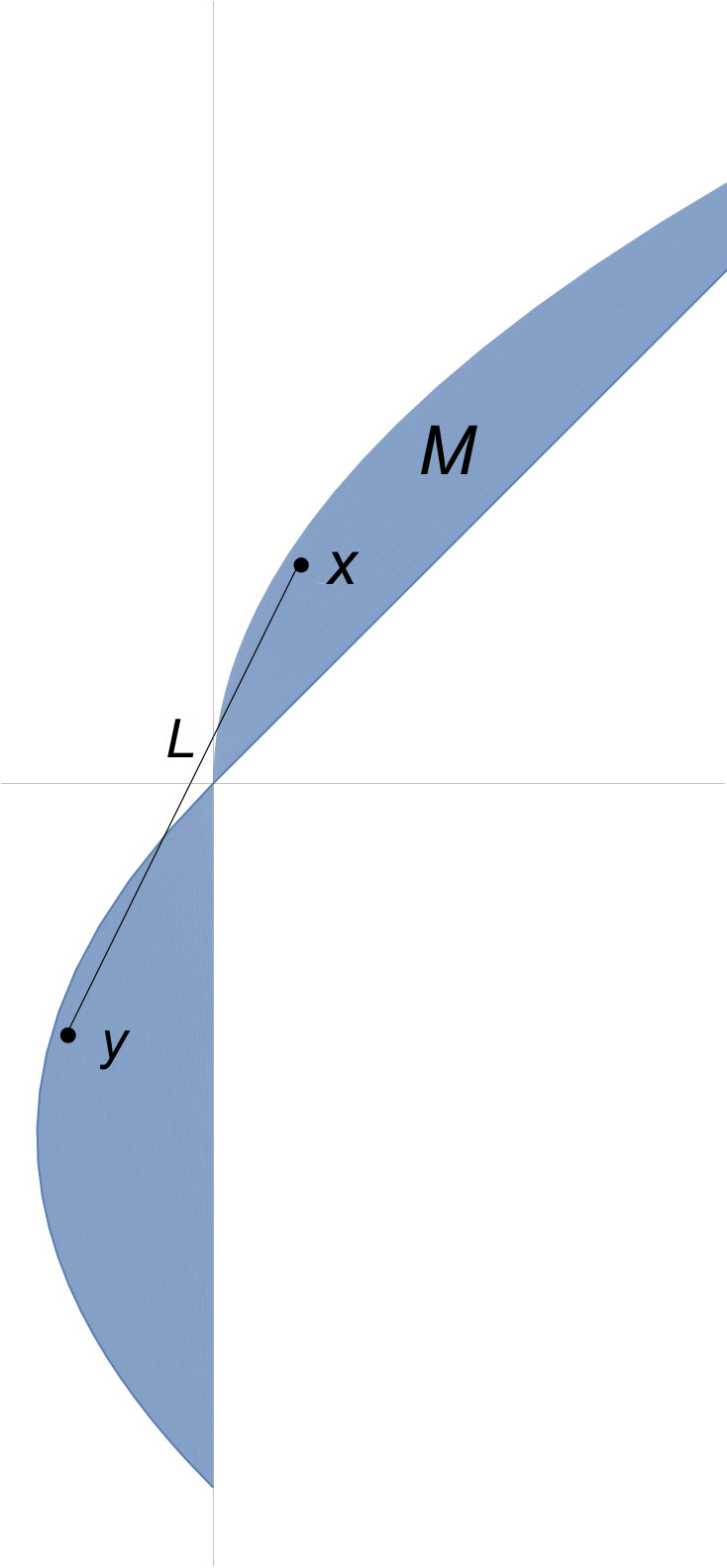 Figure 1
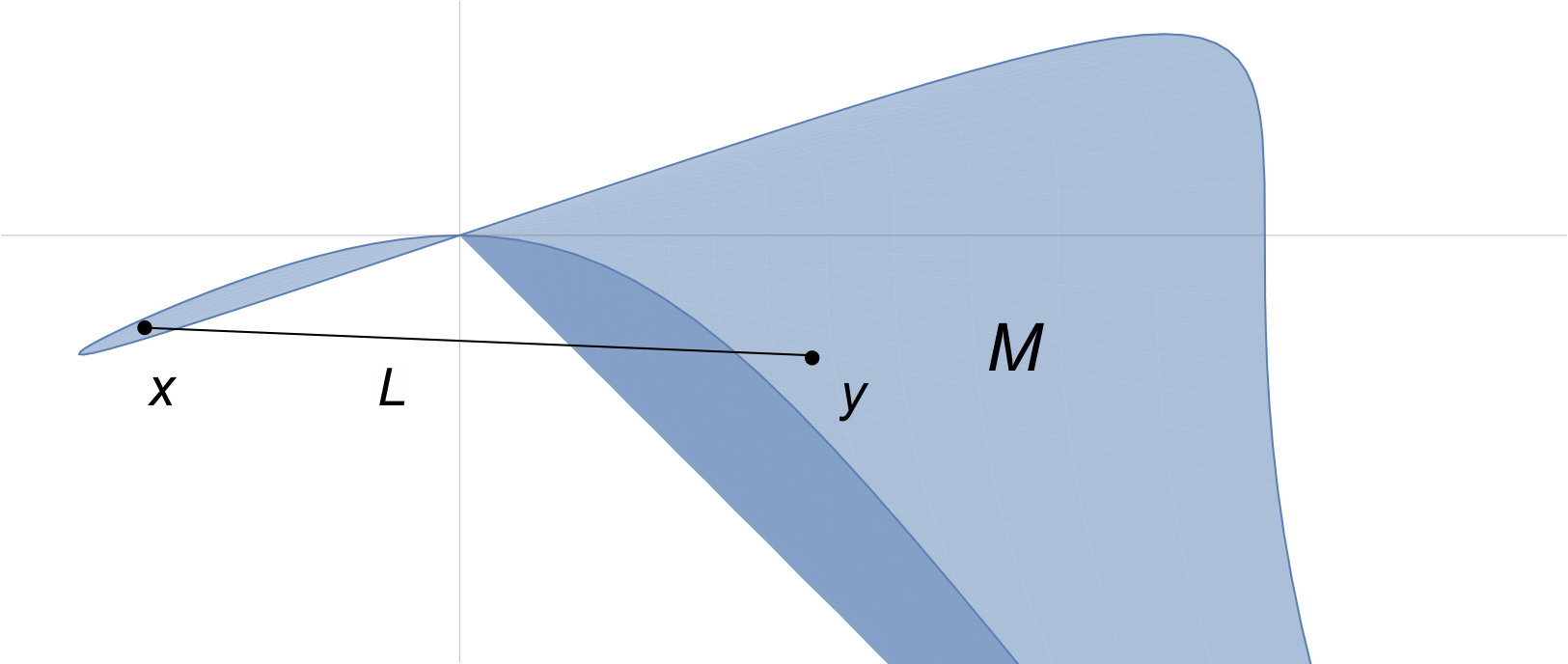 Figure 2
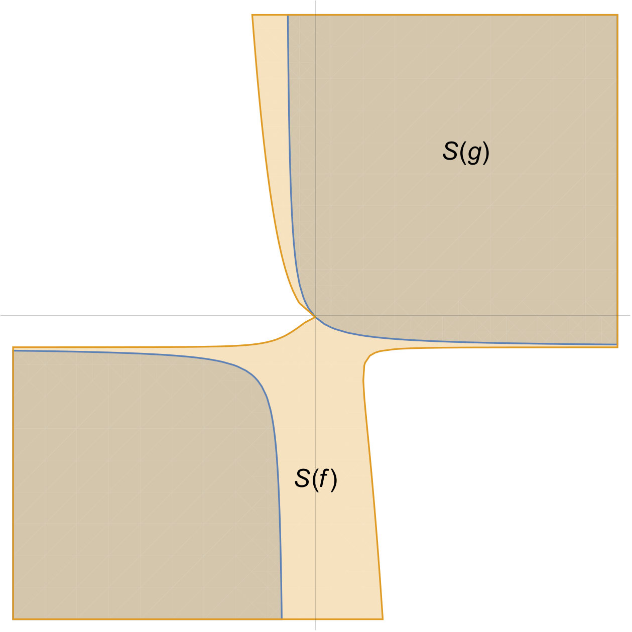 Figure 3
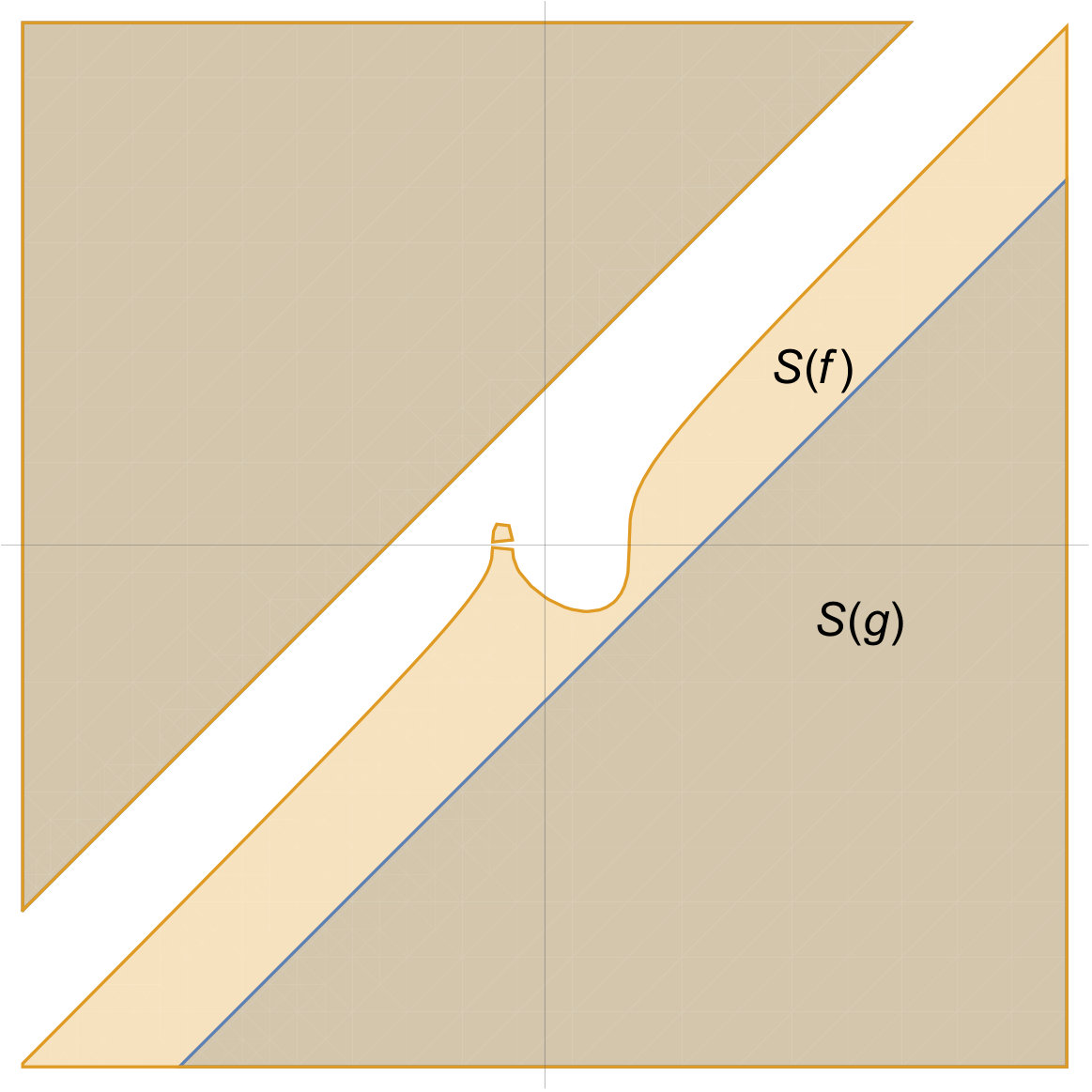 Figure 4
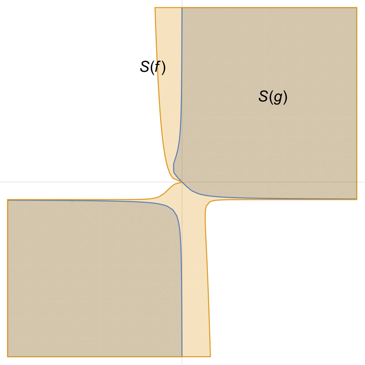 Figure 5