Flavour mixings in flux compactifications
Wilfried Buchmuller, Julian Schweizer

TL;DR
This paper explores how flux compactifications in a 6D supersymmetric SO(10) model naturally generate quark and lepton families, with flavor structures determined by zero-mode wave functions, and analyzes the resulting flavor mixing patterns.
Contribution
It introduces a flux compactification model with specific bulk multiplets that produce realistic flavor structures and discusses zero-mode wave functions' role in flavor mixing.
Findings
Zero-modes form vectorlike split multiplets for flavor phenomenology
Pattern of flavor mixing for the two heaviest SM families analyzed
Framework can be extended to three or more generations
Abstract
A multiplicity of quark-lepton families can naturally arise as zero-modes in flux compactifications. The flavour structure of quark and lepton mass matrices is then determined by the wave function profiles of the zero-modes. We consider a supersymmetric model in six dimensions compactified on the orbifold with Abelian magnetic flux. A bulk -plet charged under the provides the quark-lepton generations whereas two uncharged -plets yield two Higgs doublets. Bulk anomaly cancellation requires the presence of additional - and -plets. The corresponding zero-modes form vectorlike split multiplets that are needed to obtain a successful flavour phenomenology. We analyze the pattern of flavour mixings for the two heaviest families of the Standard Model and discuss possible generalizations to three…
Click any figure to enlarge with its caption.
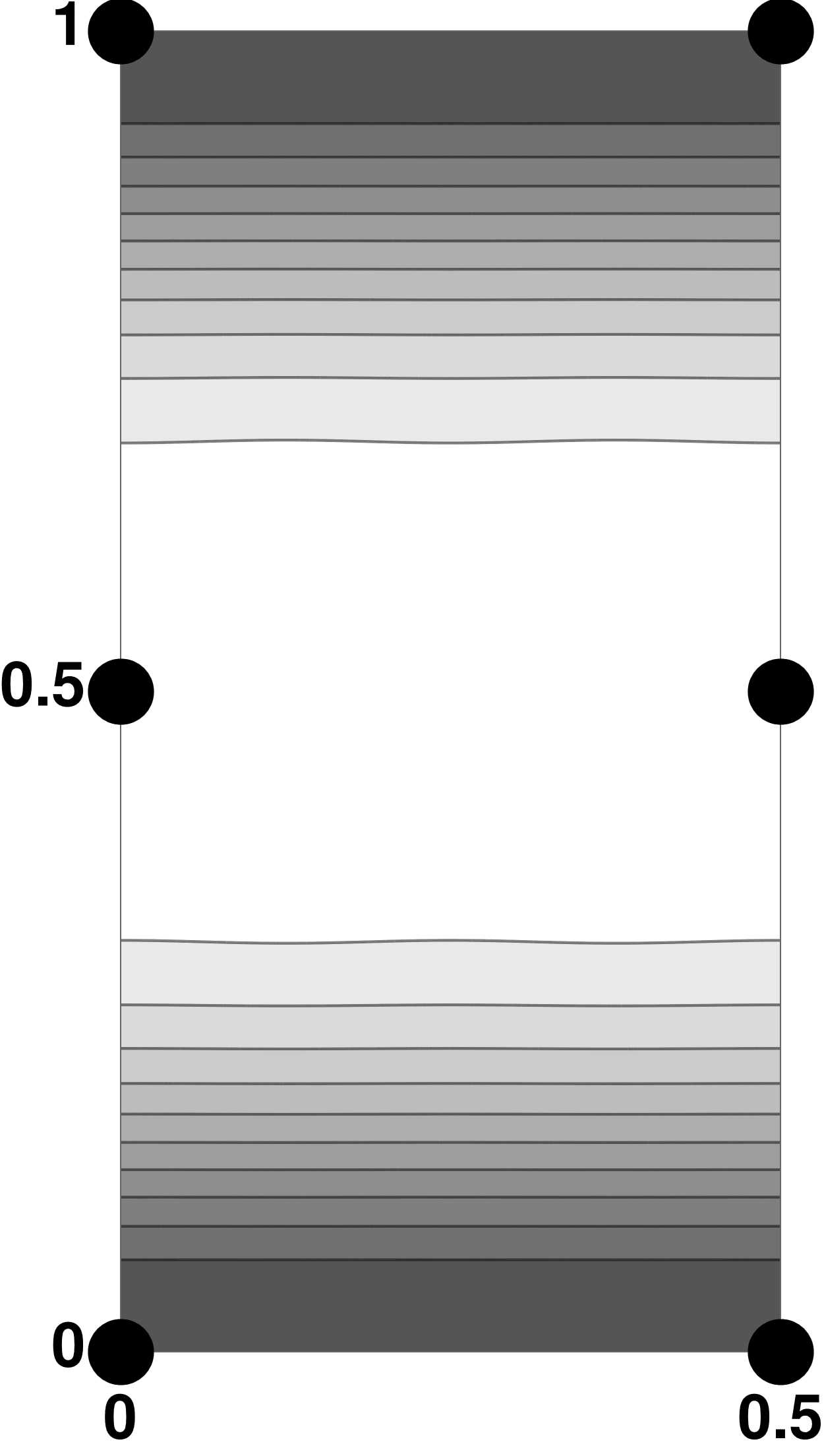 Figure 1
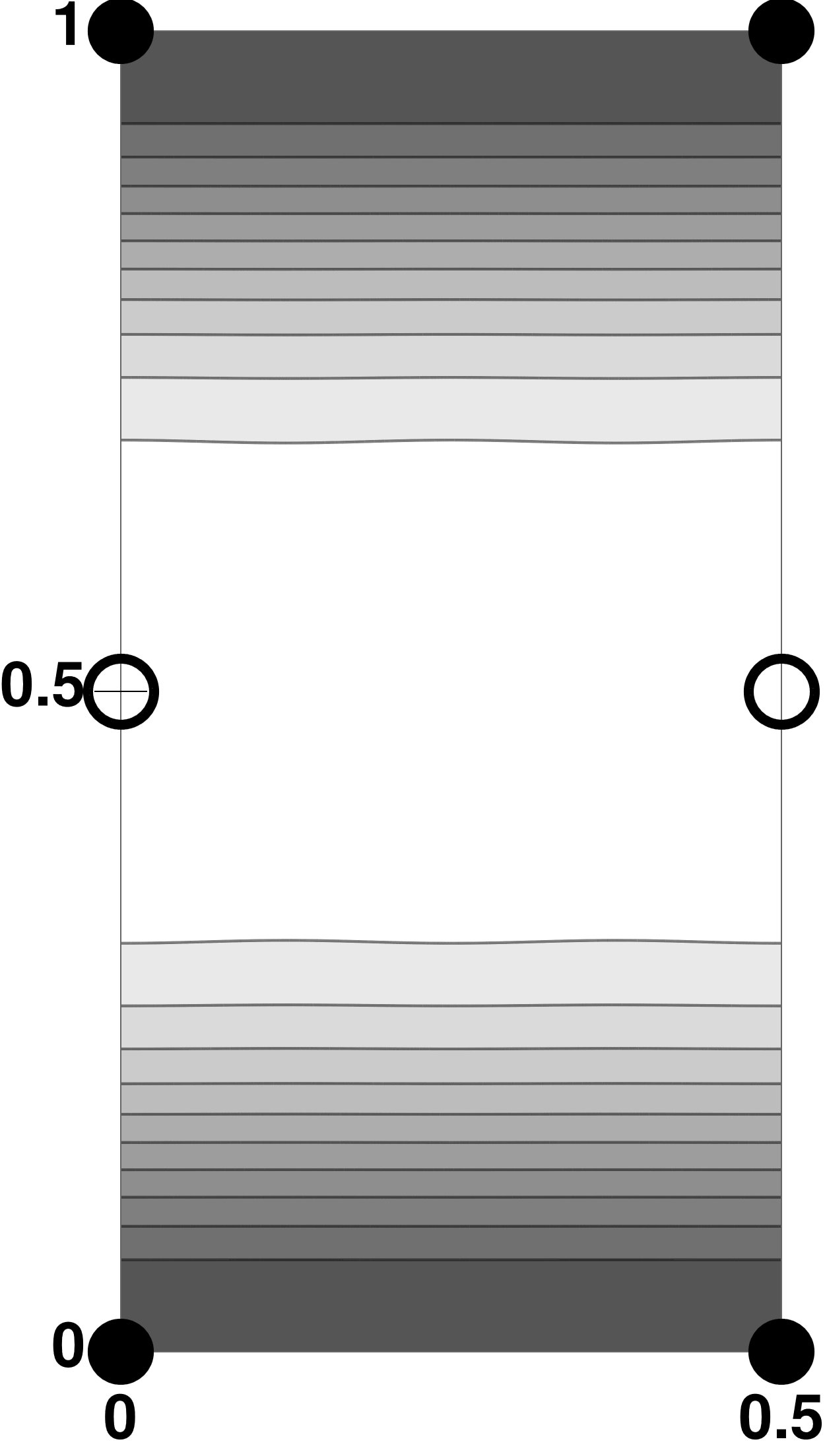 Figure 2
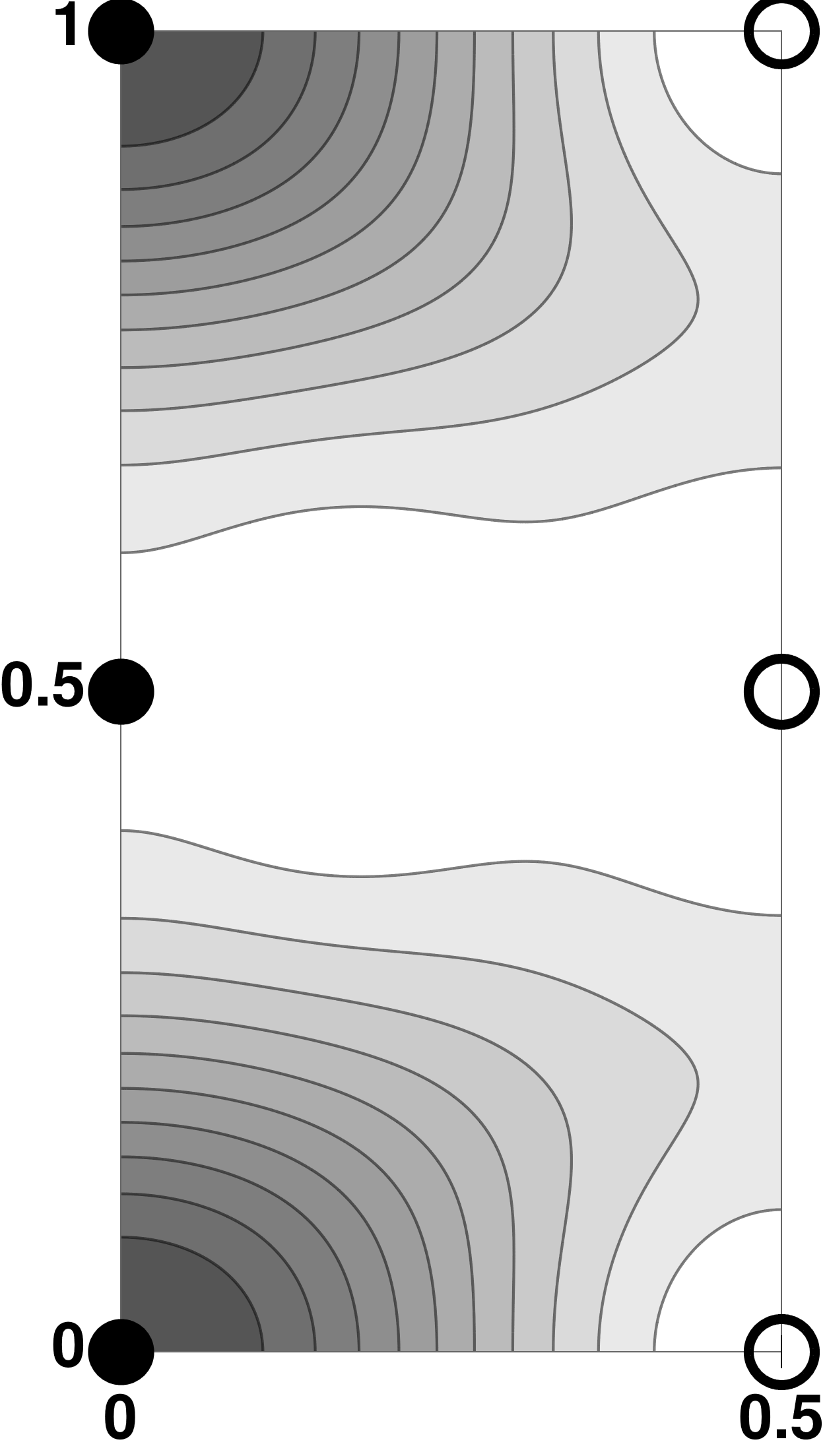 Figure 3
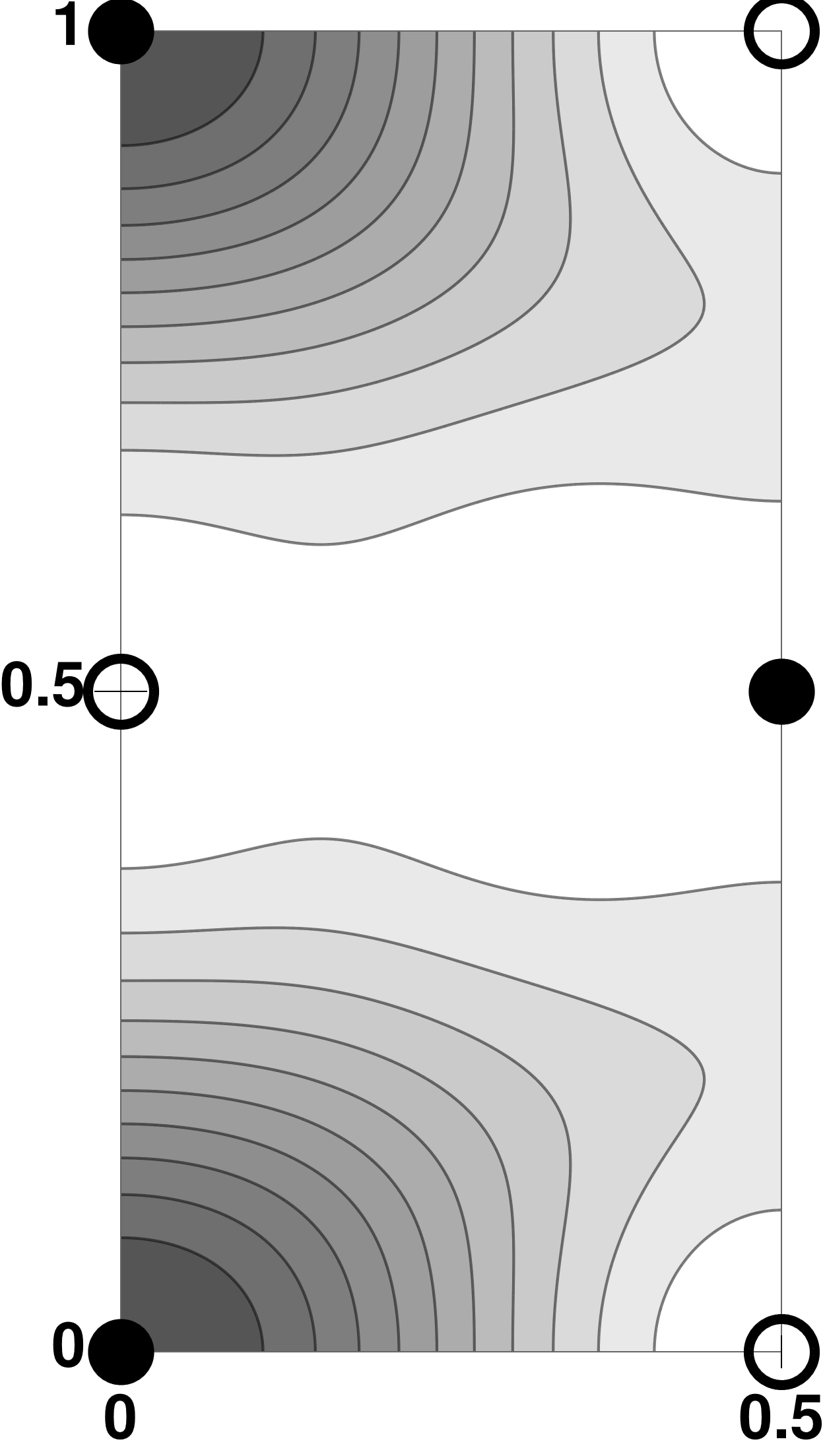 Figure 4
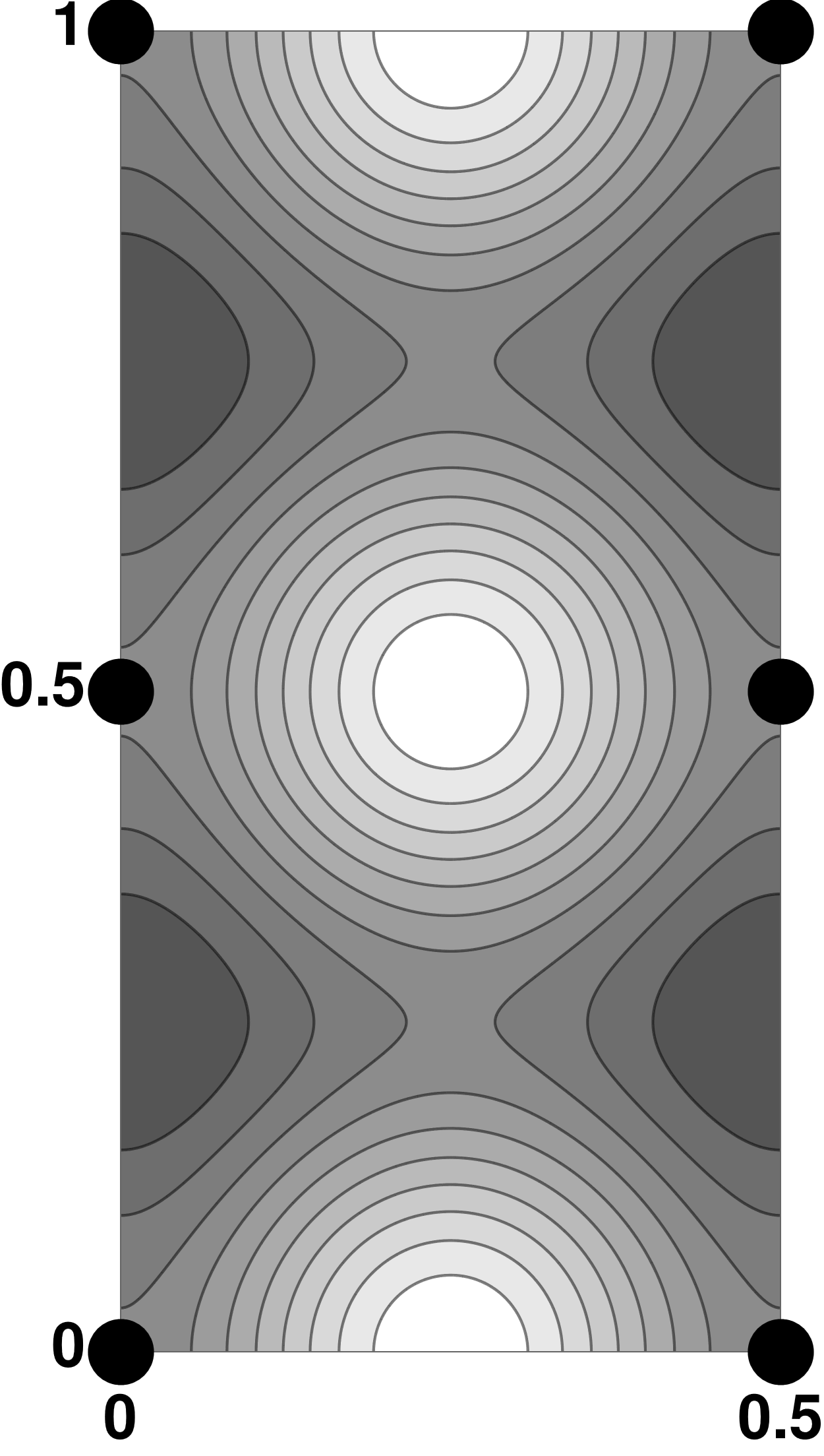 Figure 5
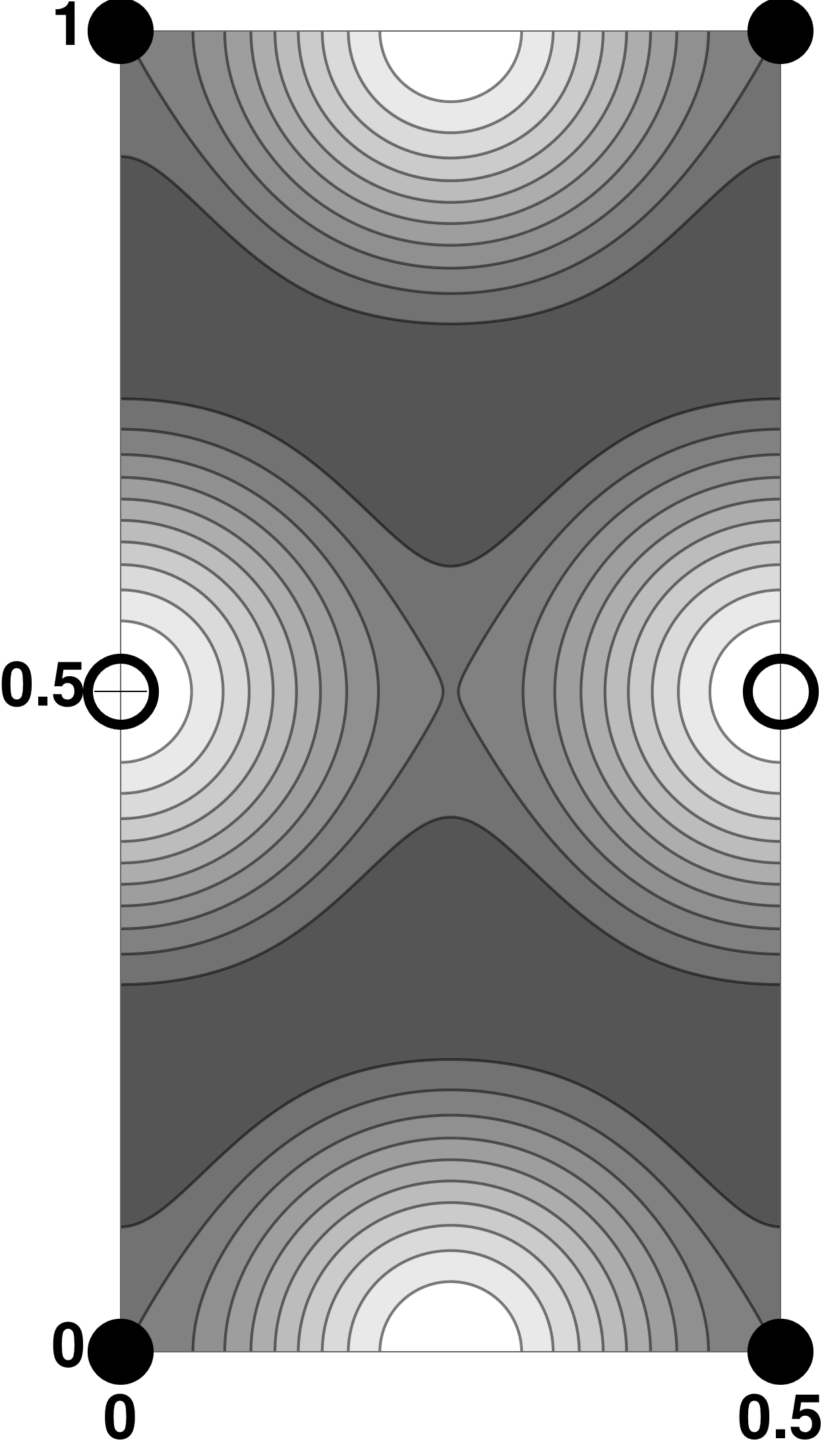 Figure 6
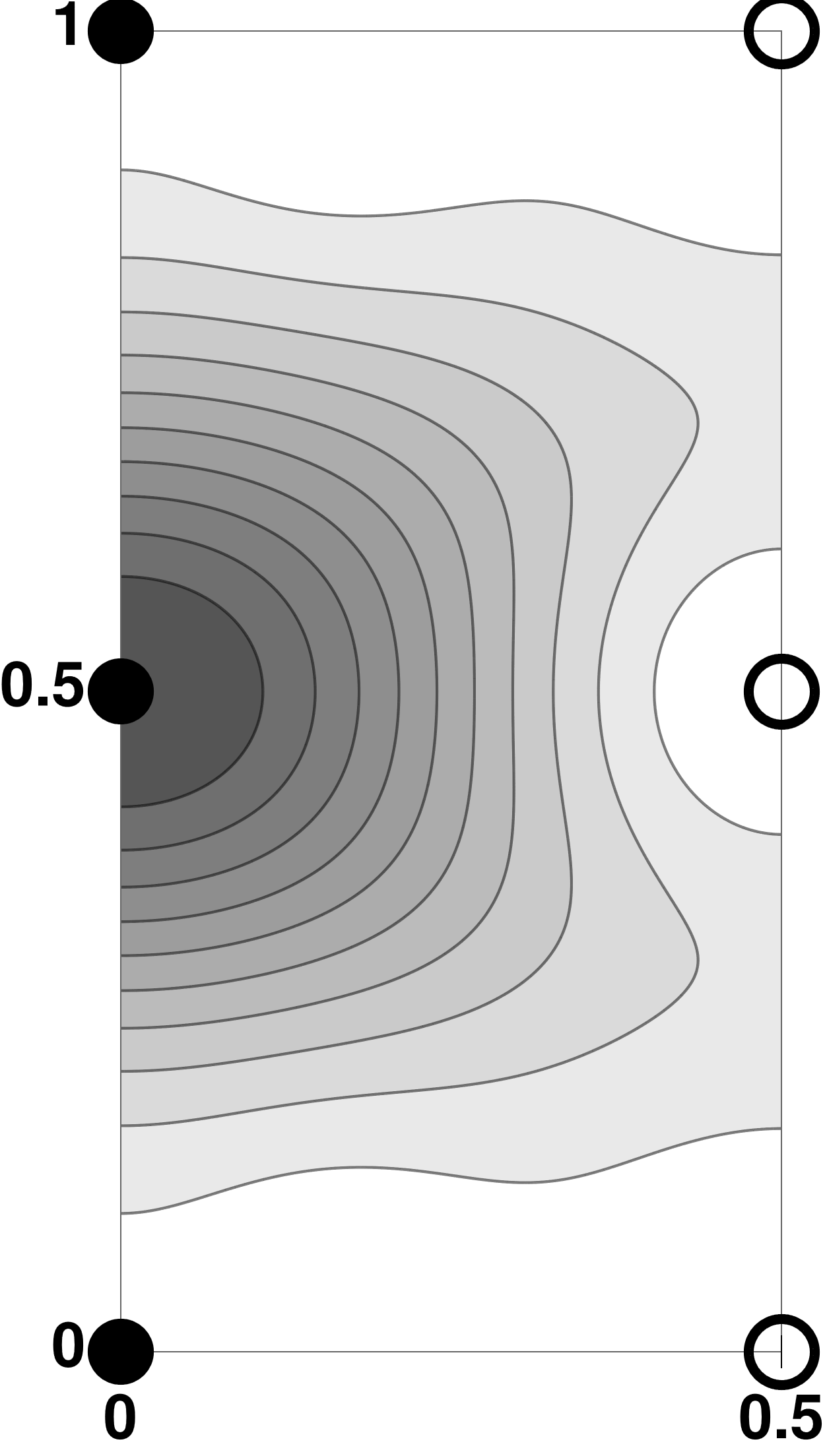 Figure 7
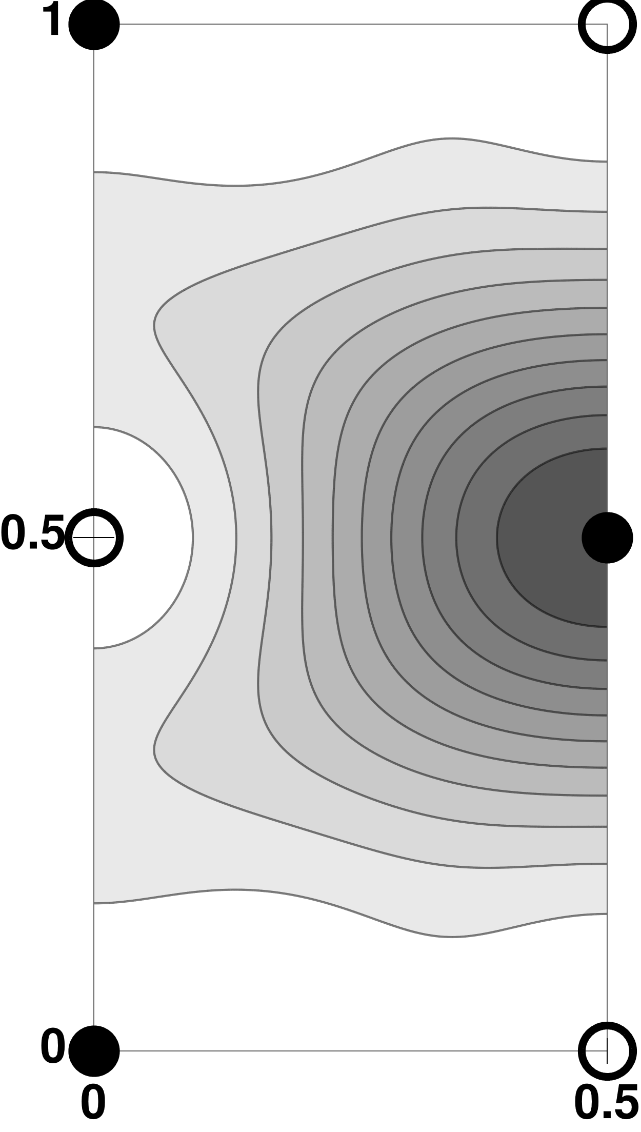 Figure 8
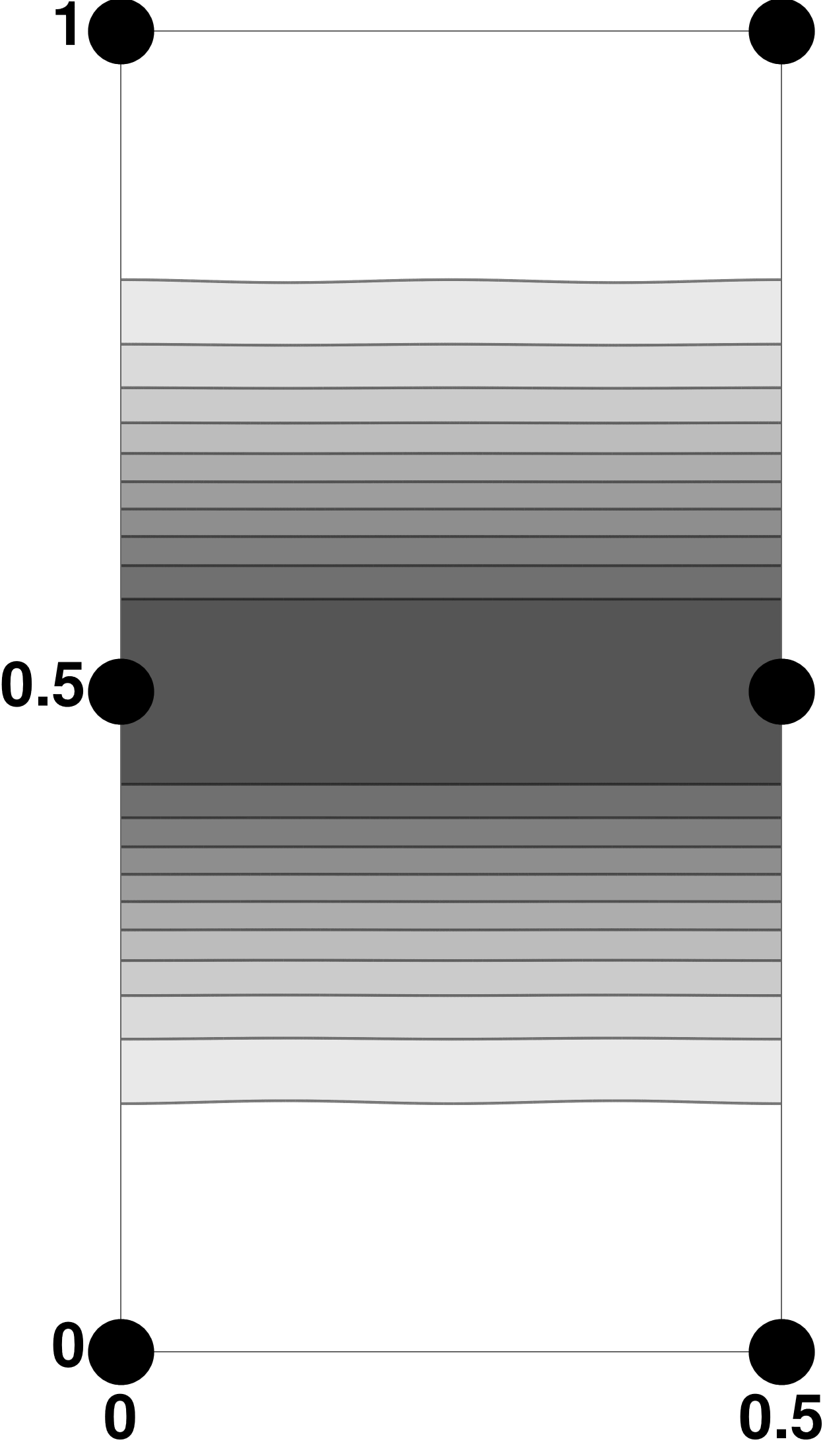 Figure 9
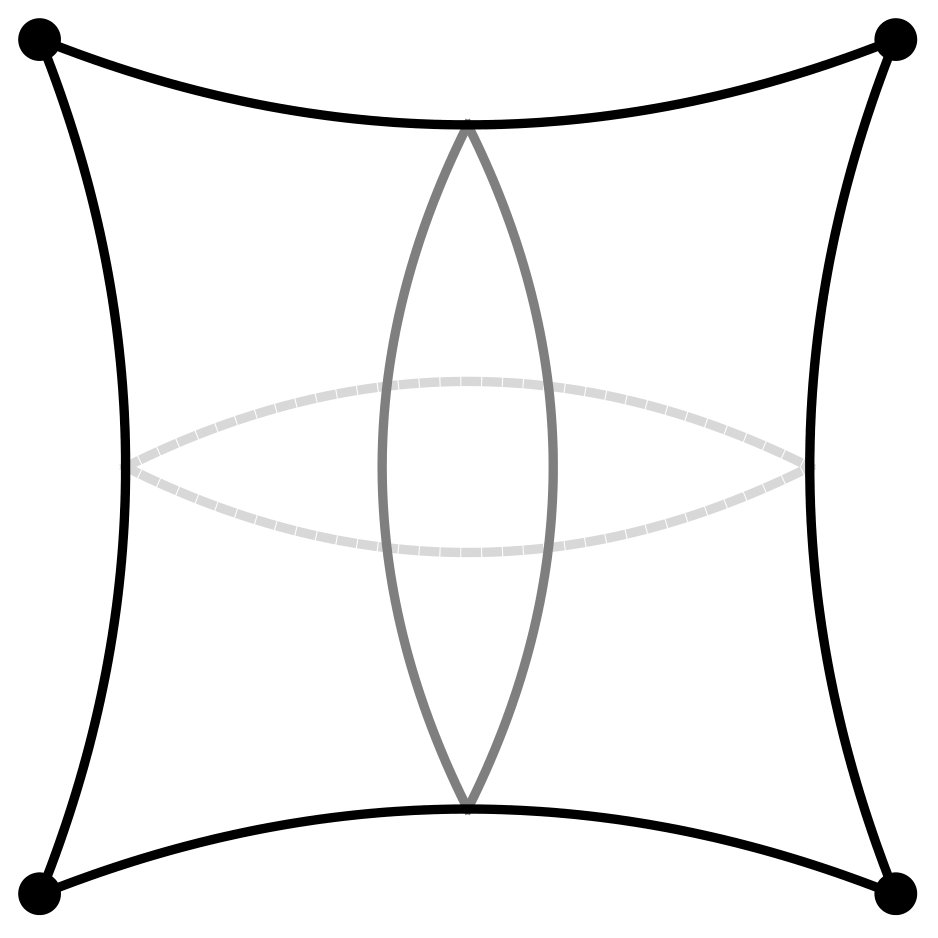 Figure 10
 Figure 11
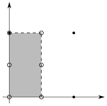 Figure 12
| Model | ||||||||
|---|---|---|---|---|---|---|---|---|
| I | + | + | ||||||
| II | + | |||||||
| III | + | |||||||
| IV |
Peer Reviews
No public reviews on file for this paper yet. If you reviewed it on a platform where reviews are public (OpenReview, ICLR, NeurIPS, ICML), you can paste yours below so the community can read it here.
Videos
No videos yet. Explain this paper in a talk, walkthrough, or lecture? Add one.
DESY 16-238
**Flavour mixings in flux compactifications
**
Wilfried Buchmuller111E-mail: [email protected] and Julian Schweizer222E-mail: [email protected]
*Deutsches Elektronen-Synchrotron DESY, 22607 Hamburg, Germany
Abstract
A multiplicity of quark-lepton families can naturally arise as zero-modes in flux compactifications. The flavour structure of quark and lepton mass matrices is then determined by the wave function profiles of the zero-modes. We consider a supersymmetric model in six dimensions compactified on the orbifold with Abelian magnetic flux. A bulk -plet charged under the provides the quark-lepton generations whereas two uncharged -plets yield two Higgs doublets. Bulk anomaly cancellation requires the presence of additional - and -plets. The corresponding zero-modes form vectorlike split multiplets that are needed to obtain a successful flavour phenomenology. We analyze the pattern of flavour mixings for the two heaviest families of the Standard Model and discuss possible generalizations to three and more generations.
1 Introduction
The explanation of the masses and mixings of quarks and leptons remains a challenge for theories which go beyond the Standard Model (SM). Interesting relations between quark and lepton mass matrices are obtained in grand unified theories (GUTs) based on the gauge groups [1], [2], [3, 4] and flipped [5, 6], and some understanding of the hierarchies between quark-lepton generations can be obtained by means of flavour symmetries [7].
Extending grand unified theories to higher dimensions offers new possibilities for symmetry breaking and the doublet-triplet splitting problem. This has been studied in particular in orbifold GUTs where the colour triplet partners of the Higgs doublets are projected out from the spectrum of massless states [8, 9, 10, 11, 12]. Orbifold GUTs can also be obtained as intermediate step towards the embedding of the Standard Model into string theories [13, 14, 15, 16].
Important progress in understanding the flavour structure of the Standard Model has also been made in the context of the heterotic string [17, 18] as well as in F-theory [19, 20, 21]. In string theory Yukawa couplings are dynamical quantities whose values depend on the vacuum structure of the theory. An interesting example are flux compactifications where the Yukawa couplings can be calculated as overlap integrals of wave functions that have non-trivial profiles in the magnetized extra dimensions [22]. In a similar way, Yukawa couplings of magnetized toroidal orbifolds have been analyzed [23, 24, 25, 26]. The resulting flavour structure depends on the number of pairs of Higgs doublets. In the simplest cases it appears difficult to obtain the measured hierarchies of quark and lepton masses [24, 25].
Magnetic flux leads to a multiplicity of chiral fermion zero-modes according to the number of flux quanta, which can be used to explain the number of quark-lepton generations [27]. Moreover, flux is an important source of supersymmetry breaking [28]. Starting from a six-dimensional orbifold GUT model [29] with gauge group , we have considered in [30] possible effects of an additional factor. Abelian magnetic flux can be used to generate a multiplicity of quark-lepton families from a charged bulk -plet. Bulk anomaly cancellation requires additional -plets and -plets that can be uncharged. The orbifold projection then leads to split multiplets, which allow for the familiar solution of the doublet-triplet splitting problem in the Higgs sector. Since the quark-lepton hypermultiplet carries charge, the scalar superpartners of quarks and leptons acquire large supersymmetry breaking masses of order the GUT scale, leading to a picture reminiscent of ‘split supersymmetry’ [31, 32].
In this paper we study the flavour structure of the orbifold GUT model [30]. The magnetic flux leads to a non-trivial profile of the quark and lepton bulk wave functions whereas the Higgs zero-modes have a constant bulk profile. Contrary to previously considered flux compactifications, Yukawa couplings arise from superpotential terms at the orbifold fixed points, i.e., from products of quark-lepton wave functions and not as volume integrals over products of quark-lepton and Higgs wave functions. Moreover, mass mixings of quarks and leptons with split multiplets occur. This offers new possibilities to obtain a realistic pattern of quark and lepton mass matrices.
The paper is organized as follows. In Section 2 we recall the needed features of the symmetry breaking in the GUT model [30] and discuss properties of the zero-mode wave functions. The main part of the paper are Sections 3 and 4. Here the structure of the quark and lepton Yukawa couplings and mass mixings is discussed, and a quantitative description is given for masses and mixings of the two heaviest SM families. Section 5 summarizes some aspects of supersymmetry breaking and the Higgs sector. The appendices A and B give some details on Wilson line breaking and the complex flavour vectors which determine Yukawa matrices and mass mixings.
2 GUT model and symmetry breaking
In this section we recall the main features of a six-dimensional GUT model previously discussed in [30]. In particular, we discuss the GUT symmetry breaking by means of Wilson lines, list all the fields relevant for flavour mixing and discuss the properties of the zero-mode wave functions that determine the Yukawa matrices and the mixings with split multiplets.
We start from supersymmetry in six dimensions with gauge symmetry, compactified on the orbifold . In addition to the -plet of vector multiplets the model contains six -plets and four -plets. For this set of bulk fields all irreducible and reducible gauge anomalies cancel [29, 30]. It is convenient to group vector multiplets into vector multiplets and chiral multiplets , and hypermultiplets into two chiral multiplets, and [33]. Note that transform in the the complex conjugate representation compared to . The origin is a fixed point under reflections, , where denotes the coordinates of the compact dimensions. Defining fields on the orbifold such that
[TABLE]
breaks supersymmetry to 4d supersymmetry at the fixed point .
The bulk symmetry can be broken to the Standard Model group by means of two Wilson lines111In Refs. [11] the breaking of was obtained by considering the orbifold . This is equivalent to the symmetry breaking on with two Wilson lines that is considered in this section.. The fixed points , are invariant under combined lattice translations and reflection: , with , , where denotes a lattice vector (see Appendix A). Demanding that fields on the orbifold satisfy the relations
[TABLE]
with matrices , given in Appendix A and parities , the gauge group is broken to the Pati-Salam subgroup and the Georgi-Glashow subgroup at the fixed points and , respectively (see Fig. 1). The surviving SM gauge group is obtained as intersection of the Pati-Salam and Georgi-Glashow subgroups of ,
[TABLE]
Group theory implies that is broken to flipped , , at .
Analogously to the vector multiplets the hypermultiplets satisfy the relations
[TABLE]
where the matrices and now depend on the representation of the hypermultiplet. The multiplets and can be decomposed into SM multiplets, and . Each of them belongs to a repesentation of as well as and is therefore characterized by two parities,
[TABLE]
The parities of the vector multiplet are fixed by the requirement that the SM gauge bosons are zero-modes. The parities of the hypermultiplets can be freely chosen subject to the requirement of anomaly cancellations. A given set of parities then defines a 4d model with SM gauge group.
Magnetic flux is generated by a background gauge field. One bulk -plet, , carries charge. The other -plets, , and , and the -plets have no charge. Each hypermultiplet leads to a ‘split multiplet’ of 4d zero-modes that have both parities positive. This allows for the wanted doublet-triplet splitting in the Higgs sector. The parities and can be chosen such that and contain the Higgs doublets and , respectively. The -plets and contain zero-modes and , respectively. Expectation values of and break , and therefore . and have down-quark quantum numbers and acquire mass by mixing with the zero-modes of the -plets and listed in Table 3 of Appendix A. The -plets and also have zero-modes with down quark quantum numbers. In Table 1 all zero-modes are listed, which are relevant for our discussion of flavour mixing.
The charged bulk -plet yields -plets of zero-modes for flux quanta, independent of the parity assignements, plus an additional split multiplet of zero-modes for which both parities are positive. The zero-modes of a charged hypermultiplet have non-trivial wave function profiles. There are four possibilies to choose a pair of parities , . Correspondingly, there are four models that differ by the parities of the SM components, and therefore the assignment of the four types of wave functions to quarks and leptons. The four models are listed in Table 2.
For our discussion of flavour mixings we choose model II where and have both parities positive. Hence, the bulk field has the decomposition
[TABLE]
For the wave functions we use the expressions given in [34]. For flux quanta they read
[TABLE]
For there are zero-modes, with . In all other cases one has zero-modes, with . The shape of the wave functions is shown in Fig. 2. The wave functions are non-zero at all fixed points. All other wave functions are non-zero at two fixed points and vanish at the other two. As we shall see in the subsequent section, this leads to a characteristic pattern of flavour mixings.
3 Flavour mixings from geometry
In this section we discuss the geometric origin of flavour mixing in our model. Supersymmetry in six dimensions does not allow for a bulk superpotential. Couplings between the bulk hypermultiplets can therefore only arise at the fixed points. There, the couplings of fields are proportional to the product of their wave functions, evaluated at the respective location. The background flux leads to a multiplicity of fermion families in our model, and each Yukawa coupling of hypermultiplets at a fixed point is therefore turned into a flavour matrix. The SM gauge quantum numbers and the Wilson line configuration determine the wave function for a given field, see Table 2. In the following we shall focus on model II.
In order to illustrate how the Yukawa matrices arise from the wave function profiles, let us consider a down-type quark Yukawa matrix. This arises at the fixed point from the term
[TABLE]
where are the family indices which label the degeneracy of of the zero-mode wave functions. The wave functions have to be evaluated at the fixed point, and we assume electroweak symmetry breaking with . From Eq. (9) and Eqs. (59), (67) one obtains the down-quark Yukawa matrix
[TABLE]
In principle, there are further contributions to the down-quark Yukawa couplings from other fixed point superpotentials. However, all operators involving the quark doublet vanish at the Pati-Salam fixed point, as they are proportional to that vanishes at due to their negative parity there. By the same reason there is neither a contribution from the Georgi-Glashow fixed point where the right-handed down quark wave functions vanish, nor from the flipped fixed point where both the quark doublets and the right-handed down quarks cannot couple. Up to higher-dimensional operators, the model II therefore predicts the down-quark Yukawa couplings uniquely.
The matrix given in Eq. (10) has some characteristic features. First of all, one of the eigenvalues vanishes,
[TABLE]
so there is only one heavy state with nonvanishing mass. This follows immediately from the fact that the matrix is a dyadic tensor build from two vectors that determine the couplings of and at the fixed point . As we shall see, a second nonvanishing mass can be obtained from the mixing with vectorlike split multiplets. Furthermore, it is interesting that the matrix (10) is complex, which is a consequence of the two nonvanishing Wilson lines. It therefore naturally incorporates CP violation.
In most cases, the Yukawa matrices have contributions from two fixed points. It is straightforward to list the lowest-dimensional operators that contribute to fermion masses at the various fixed points after and electroweak symmetry breaking,
[TABLE]
where we denote the Higgs fields in the representations of the unbroken subgroups at the various fixed points by , , , , , , , and ; , , and the vacuum expectation values of the Higgs fields are , and . We refer to the matter fields at the various fixed points by their or representation respectively, marking flipped fields with a tilde. Specifying to model II, all but six of the operators in Eq. (12) vanish because in most couplings one of the matter field wave functions is zero at the fixed point. This considerably simplifies the superpotential,
[TABLE]
The dimension-four operators give Yukawa couplings for the quarks, charged leptons and neutrinos, whereas the dimension-five operators give Majorana masses for the right-handed neutrinos.
As we showed above for the down-type quarks, the wave functions fully determine the matrix structure of the couplings. Of special note in this regard are the fields with even parities at all fixed points, and . For these, the degeneracy induced by flux quanta is -fold, so the up-quark and charged lepton Yukawa matrices derived from Eq. (13) are actually matrices.
As described in the previous section, the considered GUT model unavoidably predicts additional vectorlike states that are expected to have mass terms of order the GUT scale. Mixing them with quarks and leptons, one can obtain realistic mass matrices. First, we project the bulk -plet, , in such a way that it complements the additional and we obtained from the flux (see Table 1). Mixing with these zero-modes and , the up-quark and charged lepton Yukawa couplings turn into matrices. Next, we project two of the additional bulk -plets to a vectorlike pair of down-type quarks, , . Introducing mixing in the down-quark sector provides sufficient freedom to reproduce the measured features of quark mixing. Finally, a large number of SM singlet fields are required by the cancellation of gravitational anomalies. These can mix with the right-handed neutrinos, and with the left-handed neutrinos via nonrenormalizable operators.
The mixing of up-quarks and charged leptons with the zero-modes of occurs through bilinear mass terms at the fixed points where are contained in , and . The mass mixing terms read
[TABLE]
As for the Yukawa couplings, the mixing terms are proportional to the relevant wave function, in this case, evaluated at the respective fixed points. The mass matrices of up-quarks and charged leptons after electroweak symmetry breaking are then given by
[TABLE]
where , and . correspond to the electroweak scale, while the are assumed to be of the order of the compactification scale. At all but the flipped fixed points, and are part of the same irreducible representation, forcing with ; in addition one has the relation .
The down-quarks mix with the vectorlike pair through operators involving the Higgs field . The superpotential terms read
[TABLE]
where , and . All fixed points contribute to a mass term of order the unification scale for . With as breaking vacuum expectation value, the down-quark mass matrix becomes
[TABLE]
where we have explicitly introduced the mass scale for the nonrenormalizable terms.
A third kind of mixing appears in the neutrino sector. Gauge singlets, required by the cancellation of gravitational anomalies, can mix with the SM singlet right-handed neutrinos. These couplings involve the Higgs field . The gauge singlets can also couple to the left-handed neutrinos through a nonrenormalizable interaction, involving both and . Considering for simplicity only one singlet , one obtains for the bilinear superpotential terms
[TABLE]
all fixed points contribute to a singlet mass term . Combining the mixing terms with the Yukawa interactions (13), one obtains a Dirac neutrino mass matrix,
[TABLE]
where , and a Majorana neutrino mass matrix for the heavy sterile neutrinos,
[TABLE]
Despite the mixing with an additional sterile neutrino, the seesaw formula can still be applied to obtain the light neutrinos mass matrix
[TABLE]
Let us finally emphasize the GUT relations between the parameters. These are in particular the relations for the Yukawa couplings at the fixed point : and , as well as the relations for the mixing parameters, with .
4 The two heavy families
Let us now consider the case of two flux quanta, , and apply it to the two heaviest families of the Standard Model. We start with the down-quark mass matrix, already discussed in the previous section. As an example, we choose the parameters222We also choose , , . Note that the precise values of these parameters is not important. A change can be compensated by rescaling the superpotential parameters. The parameters are chosen to reproduce the properties of the two heaviest SM families. , , , , and . From Eq. (19) and the values of the wave functions given in Eqs. (59), (67) one obtains the matrix
[TABLE]
where the third row vector contains GUT scale masses.
It turns out that the quark and charged lepton mass matrices are all of the form
[TABLE]
with . This matrix can be reduced to a matrix by integrating out one heavy state with GUT-scale mass [29]. Let us introduce an orthonormal set of vectors with
[TABLE]
Defining two unitary matrices and by
[TABLE]
one easily verifies (),
[TABLE]
up to corrections of relative order . Clearly, the matrix in the upper-left corner is the relevant low-energy mass matrix.
Using Eq. (28) it is straightforward to integrate out the heavy state contained in the matrix (24). For a convenient choice of vectors one then finds the matrix
[TABLE]
with the mass eigenvalues
[TABLE]
The up-quark mass matrix can be obtained in the same way. We choose the additional parameters as , and with . From Eqs. (15), (58) and (59) one obtains the mass matrix
[TABLE]
After integrating out the heavy state one finds the matrix
[TABLE]
with the mass eigenvalues
[TABLE]
Diagonalizing the up- and down-quark mass matrices by biunitary transformations, one obtains from the left-handed rotation matrices the CKM matrix. We find the mixing angle . The obtained bottom, strange, top and charm masses and the CKM mixing angle agree with the measured values at the GUT scale within 5%333We take all masses and mixings angles at the GUT scale from the recent compilation [35].. Given the structure of the quark mass matrices the small mixing angle is rather surprizing. Indeed, the individual rotation angles for the diagonalization of the up- and down-quark matrices are much larger. However, since the matrices are rather similar, the mismatch is small, which leads to a small angle in the CKM matrix.
The charged lepton mass matrix is mostly determined by the parameters of the quark mass matrices. In addition we choose and . From Eq. (16) and the wave functions given in Eqs. (58), (63) one obtains the charged lepton matrix
[TABLE]
Integrating out the heavy state yields the matrix
[TABLE]
with the mass eigenvalues
[TABLE]
The neutrino sector plays a special role. Eq. (21) yields a Dirac neutrino mass matrix whereas Eq. (22) gives a matrix for the heavy sterile neutrinos. Choosing the remaining parameters as , and , , , , , and using the wave functions Eqs. (63), (67), one finds the Dirac neutrino mass matrix,
[TABLE]
and the sterile neutrino mass matrix,
[TABLE]
The seesaw formula (23) then yields the matrix for the light neutrinos
[TABLE]
with the mass eigenvalues
[TABLE]
The vanishing eigenvalue is again a consequence of the dyadic tensor structure of the neutrino Yukawa matrix. Diagonalizing the charged lepton and neutrino mass matrices one finds the MNS mixing angle . The lepton masses and the MNS mixing angle are roughly consistent with the measured values at the GUT scale [35]. Contrary to the quark sector the mixing angle is large in the lepton sector. This is a consequence of the seesaw mechanism which implies that the transitions from flavour to mass eigenstates for charged leptons and neutrinos do not compensate each other.
Having fixed the parameters of our model one could hope that changing the number of flux quanta to would yield a successful description of the Standard Model with three quark-lepton families. Unfortunately, this is not the case. In fact, the third family would remain massless. The reason is once more the dyadic structure of the Yukawa matrices. The flux compactification provides a -component complex vector for each of the six SM fields at the four fixed points (see Table 2). However, due to the presence of two Wilson lines, for five SM fields these vectors vanish at two fixed points. Hence many Yukawa matrices, which are products of two vectors, and mixings with the additional vector-like states vanish. As a consequence, mass matrices with full rank can be obtained for but not for .
There are several ways to avoid this problem. The simplest possibility is to have more than one bulk -plet that feels the magnetic flux, for instance one -plet with charge one and one -plet with charge two in the case of one flux quantum. Alternatively, one could start with a smaller bulk gauge group such as so that one Wilson line is enough to achieve symmetry breaking to the Standard Model. Finally, it is conceivable that not all quarks and leptons are zero-modes from magnetic flux and that some of them result from split bulk fields or from fields localized at some fixed points. These possibilities will be studied in future work.
5 Supersymmetry breaking and Higgs sector
For completeness, we summarize in this section some other aspects of the considered GUT model, which are of phenomenological interest. The Abelian magnetic flux breaks supersymmetry. Since the matter hypermultiplet carries charge, scalar quarks and leptons acquire universal masses of the order of the compactification scale, which corresponds to the GUT scale [28, 36],
[TABLE]
where is the number of flux quanta and is the volume of the compact dimensions. The magnetic flux together with a nonperturbative superpotential at the fixed points can stabilize the compact dimensions [36], and it is possible to obtain Minkowski or metastable de Sitter vacua [37] with small cosmological constant. In these vacua the vector boson , the moduli and the axions are all heavy [38],
[TABLE]
The expectation values of the moduli F-terms are of the order of the gravitino mass. Since the moduli dependence of the gauge kinetic terms is known [38], one easily obtains for the gaugino masses
[TABLE]
whereas the SM gauge bosons are massless by construction.
At tree-level the two Higgs fields and are massless since they originate from bulk -plets that do not feel the magnetic flux. Also the higgsinos are massless since they are protected by a Peccei-Quinn-type symmetry. One may worry whether it is possible to consistently extend such a theory up to the GUT scale. In fact, this is known not to be the case for split supersymmetry or high-scale supersymmetry because of vacuum instability [39]. On the contrary, for a two-Higgs doublet model, with or without higgsinos, an extrapolation to the GUT scale is possible [40] for stable or metastable vacua [41]. This implies constraints on the masses of the heavy neutral scalar and pseudoscalar as well as charged Higgs bosons , , , respectively, and on the ratio of vacuum expectation values,
[TABLE]
Solutions of the two-loop renormalization group equations of gauge and Yukawa couplings show gauge coupling unification at a scale . At LHC energies the main hope for new discoveries lies on additional heavy Higgs bosons and higgsinos with masses .
A large scale of supersymmetry breaking, like the GUT scale that lies many orders of magnitude above the electroweak scale, reintroduces the ‘hierarchy problem’. Is an enormous fine tuning of parameters needed to keep the Higgs bosons at the electroweak scale once quantum corrections are included? This is certainly the case in the effective 4d theory if only zero-modes are taken into account in the loop diagrams. However, the situation might be different if the virtual states are extended to the whole Kaluza-Klein tower. A well known example is the mass of a Wilson line for an Abelian 6d gauge field compactified on a torus. After some regularization, one obtains a Wilson line mass of the order of the inverse size of the compact dimensions [42]. Remarkably, as was recently shown, in the presence of magnetic flux the one-loop quantum corrections to the Wilson line mass vanish [43]. This suggests that magnetic flux may provide a partial protection of scalar masses w.r.t. quantum corrections. However, the applicability to electroweak symmetry breaking in the considered GUT model remains to be investigated.
6 Summary and conclusions
Supersymmetric grand unified theories in higher dimensions provide an attractive ultraviolet completion of the Standard Model. An example is the six-dimensional model with magnetic flux considered in this paper, which itself may have an embedding into string theory. An orbifold compactification to four dimensions with two Wilson lines can break the six-dimensional gauge symmetry to the Standard Model gauge group. The quark-lepton families arise as zero-modes of complete -plets due to the magnetic flux, whereas two Higgs doublets are obtained as split multiplets from bulk -plets. Additional bulk - and -plets lead to further split multiplets that can mix with the complete quark-lepton -plets.
After describing the symmetry breaking and the quantum numbers of the zero-modes, we have analyzed the Yukawa couplings and the bilinear mixings of the zero-modes. In many flux compactifications, where also the Higgs fields feel the magnetic flux, Yukawa couplings arise from overlap integrals of bulk wave functions. On the contrary, in the model under consideration Yukawa couplings and mass mixings are superpotential terms that can arise at the orbifold fixed points. The entire flavour structure is then contained in complex vectors in flavour space, one for each SM representation at each fixed point. These vectors are a prediction of the flux compactification. They determine the mixings with split multiplets and their products yield the Yukawa matrices.
We have shown that this pattern of flavour mixing can account for masses and mixings of the two heaviest Standard Model families. The mass hierarchies are either due to a hierarchy of Yukawa couplings or to relative importance of Yukawa couplings and mass mixings. Starting generically from large flavour mixings, the CKM mixing turns out to be small due to the small mismatch of the rotation matrices for up- and down-quark mass matrices. On the other hand, the seesaw mechanism distinguishes between the charged lepton and the neutrino mass matrices, and the MNS mixing therefore remains large. It turned out that the two-flavour model cannot be extended to a three-flavour model in a straightforward way. Due to the dyadic structure of the Yukawa matrices and the presence of two Wilson lines, too many terms vanish that would be allowed by the gauge symmetries, and the lightest quark-lepton family remains massless. As briefly described in the previous section, there are several ways to avoid this problem. The investigation of these possibilities is left for future work.
Let us finally compare the pattern of flavour mixings described in this paper with successful flavour models of Frogatt Nielsen type (see, for instance, [44, 45, 46, 47]). In these models the entries of the mass matrices are powers of a small parameter, and therefore small. The powers are determined by the charges of the Standard Model fields. Choosing appropriate charges one obtains hierarchical masses and small mixings in the quark sector. The lepton sector is different due to the seesaw mechanism. Mass hierarchies in the Dirac neutrino mass matrix and the sterile neutrino mass matrix can compensate each other, leading to small mass ratios and large mixings for the light neutrinos. On the contrary, in flux compactifications one starts from mass matrices with large entries, which have rank one due to the dyadic structure of the Yukawa matrices, and therefore only one massive family. Smaller Yukawa terms and mixing with split multiplets yields small corrections and increases the rank. CKM mixings in the quark sector are small due to the small mismatch between the rotation matrices of up- and down-quark mass matrices. The neutrino sector is again different because of the seesaw mechanism and large MNS mixings remain. The two pictures of the origin of the flavour structure in the Standard Model are complementary to each other. Mass matrices of Frogatt Nielsen-type have been obtained in heterotic string compactifications (see, for instance, [50]) as well as F-theory compactifications (see, for instance, [19]). It will be interesting to understand the connection to string theory compactifications that realize large flavour mixings as in the flux compactification described in this paper.
Acknowledgments
We thank Markus Dierigl and Fabian Ruehle for valuable discussions. This work was supported by the German Science Foundation (DFG) within the Collaborative Research Center (SFB) 676 “Particles, Strings and the Early Universe”.
Appendix A Wilson line breaking on orbifolds
The breaking of to the Standard Model gauge group by boundary conditions is often based on the orbifold [11]. For completeness, we recall the equivalent description based on with two Wilson lines in the following.
The torus is obtained by identifying points which differ by a lattice vector, i.e. (see Fig. 3),
[TABLE]
Further identifying points that are related by a rotation of around the origin,
[TABLE]
one obtains the orbifold . The orbifold has four fixed points,
[TABLE]
where
[TABLE]
In an orbifold field theory one needs an embedding of the space group into field space (see, for instance, [48]) which is defined on the covering space . The corresponding transformations act linearly in field space. On the fundamental domain of the orbifold the fields then satisfy certain boundary conditions.
Using the reflection to break 6d supersymmetry to 4d supersymmetry and considering the fields even under reflection, the embedding of the space group into the gauge fields is defined by
[TABLE]
where the are matrices with
[TABLE]
In addition, one has
[TABLE]
with , . As the subscripts indicate, the matrices can be chosen such that is broken to the Pati-Salam and the Georgi-Glashow subgroups at and , respectively. For hypermultiplets one has
[TABLE]
where the matrices depend on the representation of , and the parities can be chosen independently for each hypermultiplet.
The embedding (49), (52) of the translations into field space imply that is broken to the corresponding subgroups at the fixed points,
[TABLE]
The multiplets and can be decomposed into SM multiplets, , . Each of them belongs to a representation of as well as and is therefore characterized by two parities,
[TABLE]
The matrices and have been explicitly given in [11] for the fundamental representation. At a fixed point each representation can be decomposed into representations of the unbroken subgroup, and the matrices can be written as linear combinations of projection operators onto these representations. One finds for the -, - and -plet, respectively (see [49]),
[TABLE]
Using these relations the parities in Tables 1,2 can be easily determined.
In Table 1 we have listed parities and zero-modes for all fields that are relevant for the Yukawa couplings and the mixings of split multiplets with the -plets of zero-modes. For completeness we list parities and zero-modes for the gauge fields and the -plets and in Table 3.
Appendix B Vectors in flavour space
The flavour structure of our model is entirely determined by the values of the wave functions at the various fixed points, . The degeneracy index labels idependent fields, which means we can interpret the set of wave functions with given parities as a vector in flavour space,
[TABLE]
In this appendix we give the explicit values of these vectors for flux quanta evaluated at the fixed points.
Right-handed up-quarks and electrons are states with even parity at all fixed points. Therefore, their wave function does not vanish at any fixed point. The four vectors in flavour space read
[TABLE]
They are three-vectors because the are -fold degenerate.
The left-handed quark doublet’s distribution in the internal space is given by . Their wave function is non-zero at two fixed points only,
[TABLE]
The up-quark Yukawa coupling matrix is a linear combination of two matrices which are obtained as dyadic products of flavour space vectors,
[TABLE]
Note that this matrix has rank two, independent of the dimensionality of the flavour space vectors. Mixing with the additional state is governed by a linear combination of the , which were given in Eq. (58),
[TABLE]
This gives the overall up-quark mass matrix
[TABLE]
The numerical values for an example parameter set are given in Eq. (31).
Right-handed charged leptons have the same field profile as right-handed up quarks. However, the left-handed lepton fields are given by the wave function . They are present at the and flipped fixed points,
[TABLE]
Again, the Yukawa couplings follow from a linear combination of dyadic products,
[TABLE]
while the mixing with the additional state is given by the vectors ,
[TABLE]
GUT relations imply , .
The down-quark mass terms are
[TABLE]
where is a dyadic product. The wave function values for right-handed down quarks are
[TABLE]
while those for the left-handed quarks were already given in Eq. (59) The coupling between and the is
[TABLE]
while the coupling between the and is
[TABLE]
The Dirac neutrino mass matric reads
[TABLE]
with the Yukawa matrix given by the dyadic product of the vectors given in Eq. (63) and Eq. (67). The mixing with the singlet scalar ,
[TABLE]
is also governed by the values in Eq. (63).
Finally, the Majorana mass matrix for the sterile neutrinos is
[TABLE]
The corresponding mass matrix reads
[TABLE]
where the are already defined in Eq. (67). The same flavour space vectors govern the mixing with the sterile neutrino
[TABLE]
This explicit presentation showcases that the entire flavour sector is determined by the four sets of wave functions. These determine flavour space vectors when evaluated at the fixed points. All relevant numerical values were presented in Eqs. (58), (59), (63) and (67).
The reference list from the paper itself. Each links out to its DOI / PubMed record.
- 1[1] J. C. Pati and A. Salam, “Lepton Number as the Fourth Color,” Phys. Rev. D 10 (1974) 275 Erratum: [Phys. Rev. D 11 (1975) 703].
- 2[2] H. Georgi and S. L. Glashow, “Unity of All Elementary Particle Forces,” Phys. Rev. Lett. 32 (1974) 438.
- 3[3] H. Georgi, “The State of the Art—Gauge Theories,” AIP Conf. Proc. 23 (1975) 575.
- 4[4] H. Fritzsch and P. Minkowski, “Unified Interactions of Leptons and Hadrons,” Annals Phys. 93 (1975) 193.
- 5[5] S. M. Barr, “A New Symmetry Breaking Pattern for SO(10) and Proton Decay,” Phys. Lett. 112B (1982) 219.
- 6[6] J. P. Derendinger, J. E. Kim and D. V. Nanopoulos, “Anti-SU(5),” Phys. Lett. 139B (1984) 170.
- 7[7] C. D. Froggatt and H. B. Nielsen, “Hierarchy of Quark Masses, Cabibbo Angles and CP Violation,” Nucl. Phys. B 147 (1979) 277.
- 8[8] Y. Kawamura, “Triplet doublet splitting, proton stability and extra dimension,” Prog. Theor. Phys. 105 (2001) 999 [hep-ph/0012125].