Asymptotic and bootstrap tests for the dimension of the non-Gaussian subspace
Klaus Nordhausen, Hannu Oja, David E. Tyler, Joni Virta

TL;DR
This paper introduces asymptotic and bootstrap statistical tests to accurately determine the dimension of the non-Gaussian subspace in data, enhancing the effectiveness of non-Gaussian component analysis.
Contribution
It develops new asymptotic and bootstrap testing procedures for the subspace dimension in non-Gaussian component analysis using FOBI.
Findings
Tests perform well in simulations
Bootstrap method improves accuracy in finite samples
Provides reliable dimension estimation in practice
Abstract
Dimension reduction is often a preliminary step in the analysis of large data sets. The so-called non-Gaussian component analysis searches for a projection onto the non-Gaussian part of the data, and it is then important to know the correct dimension of the non-Gaussian signal subspace. In this paper we develop asymptotic as well as bootstrap tests for the dimension based on the popular fourth order blind identification (FOBI) method.
Click any figure to enlarge with its caption.
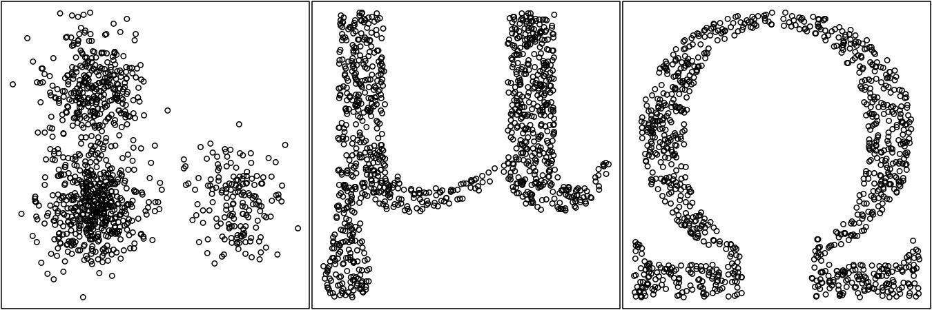 Figure 1
| Asy | Boot | Asy | Boot | Asy | Boot | |
|---|---|---|---|---|---|---|
| 500 | 0.040 | 0.128 | 0.003 | 0.031 | 0.001 | 0.012 |
| 1000 | 0.149 | 0.252 | 0.004 | 0.058 | 0.000 | 0.016 |
| 2000 | 0.403 | 0.466 | 0.027 | 0.068 | 0.000 | 0.024 |
| 5000 | 0.950 | 0.950 | 0.040 | 0.059 | 0.001 | 0.011 |
| 10000 | 0.999 | 0.999 | 0.053 | 0.058 | 0.002 | 0.010 |
| Asy | Boot | Asy | Boot | Asy | Boot | |
|---|---|---|---|---|---|---|
| 500 | 0.577 | 0.328 | 0.050 | 0.065 | 0.000 | 0.008 |
| 1000 | 0.997 | 0.964 | 0.073 | 0.056 | 0.002 | 0.008 |
| 2000 | 1.000 | 1.000 | 0.057 | 0.049 | 0.002 | 0.016 |
| 5000 | 1.000 | 1.000 | 0.068 | 0.064 | 0.004 | 0.018 |
| 10000 | 1.000 | 1.000 | 0.050 | 0.046 | 0.050 | 0.046 |
| Asy | Boot | Asy | Boot | Asy | Boot | |
|---|---|---|---|---|---|---|
| 500 | 0.715 | 0.796 | 0.024 | 0.051 | 0.001 | 0.015 |
| 1000 | 0.993 | 0.995 | 0.020 | 0.034 | 0.000 | 0.013 |
| 2000 | 1.000 | 1.000 | 0.036 | 0.044 | 0.006 | 0.016 |
| 5000 | 1.000 | 1.000 | 0.042 | 0.041 | 0.003 | 0.011 |
| 10000 | 1.000 | 1.000 | 0.043 | 0.042 | 0.005 | 0.012 |
Peer Reviews
No public reviews on file for this paper yet. If you reviewed it on a platform where reviews are public (OpenReview, ICLR, NeurIPS, ICML), you can paste yours below so the community can read it here.
Videos
No videos yet. Explain this paper in a talk, walkthrough, or lecture? Add one.
Asymptotic and bootstrap tests for the dimension of the non-Gaussian subspace
Klaus Nordhausen, Hannu Oja, David E. Tyler and Joni Virta K. Nordhausen, Hannu Oja and J. Virta are with the Department of Mathematics and Statistics, University of Turku, Turku, FIN-20014, Finland (e-mail: [email protected])D.E. Tyler is with the Department of Statistics, The State University of New Jersey, Piscataway, US.
Abstract
Dimension reduction is often a preliminary step in the analysis of large data sets. The so-called non-Gaussian component analysis searches for a projection onto the non-Gaussian part of the data, and it is then important to know the correct dimension of the non-Gaussian signal subspace. In this paper we develop asymptotic as well as bootstrap tests for the dimension based on the popular fourth order blind identification (FOBI) method.
Index Terms:
Fourth order blind identification (FOBI), independent component analysis, non-Gaussian component analysis.
I Introduction
Throughout the paper we assume the Non-Gaussian Component Analysis (NGCA) model, that is, is a random sample from the distribution of
[TABLE]
where and , is nonsingular, , and , and are independent random vectors, is non-Gaussian and is Gaussian. For non-Gaussian , there is no such that has a normal distribution. For a Gaussian , has a normal distribution for all . The idea then is, based on the observations , to make inference on the unknown , , and estimate the non-Gaussian signal and Gaussian noise subspaces determined by and , respectively. In the literature it is often preassumed that the dimension is known. In this short note we develop tests for that are based on the matrix of fourth moments used in fourth order blind identification (FOBI).
The model can also be written as
[TABLE]
where now and have ranks and , respectively. The independent random vectors and represent the signal and noise parts of . Note that and are identifiable only up to postmultiplication by and orthogonal matrices, respectively. If and the components of are independent, the model is called independent component model, is then identified up to the signs and permutation of its columns. Inference on or its inverse, the unmixing matrix , is then known as independent component analysis (ICA). [1] and [2] assumed independent components but allowed ; we call this approach non-Gaussian independent component analysis (NGICA). In our model there is no restriction on the number of Gaussian components and the non-Gaussian signal components can be dependent of each other. The Gaussian Mixture Models (GMM) with equal covariance matrices and groups and multivariate skew-normal distributions (), for example, are included in this wider model. Our definition of the NGCA model is as in [3] and originally suggested in [4]. For recent contributions and references for NGCA but always with known , see e.g. [5] and [6].
In the independent component analysis (ICA) the fourth-order blind identification (FOBI) by [7] uses the regular covariance matrix
[TABLE]
and the scatter matrix based on fourth moments
[TABLE]
where , and finds an unmixing matrix such that
[TABLE]
for some diagonal matrix . and then provide the eigenvectors and eigenvalues of and , . If in the independent component model the fourth moments of are distinct, is uniquely defined up to signs and permutations of its rows and has independent components with distributions of (up to signs). For a Gaussian , . The matrix also lists the eigenvalues of the symmetric matrix
[TABLE]
Our test constructions for the dimension of the signal space in the wider NGCA model are based on the estimated eigenvalues of . The test statistics were proposed already in [8] for the NGICA model but without a careful analysis of their limiting distributions.
The plan in this paper is as follows. In Section II our test statistic for testing whether the dimension of the signal space is is introduced. The asymptotic and bootstrap test versions are provided in Sections III and IV, respectively. Also the estimate based on the asymptotic test is discussed. The two strategies are compared in simulations in Section V and the paper ends with a discussion on alternative tests. The proofs are provided in the Appendix.
Throughout the paper we use the following notation. The first and second moments of the eigenvalues of positive definite and symmetric are denoted by
[TABLE]
and the variance of the eigenvalues is . We write for the set of matrices with orthonormal columns, .
II Test statistic for the dimension
Recall that is a random sample from a distribution of where is non-singular, , and . Further where and are independent, is non-Gaussian and is Gaussian. We also need to assume that the fourth moments exist and for all , . This is a bit stronger assumption than non-Gaussianity of . With unknown , we then wish to test the null hypothesis
[TABLE]
stating that the dimension of the signal space is .
Natural estimates of , and are
[TABLE]
[TABLE]
and , respectively. To test the null hypothesis , we use the test statistic
[TABLE]
If
[TABLE]
then .
Note that [9] used to test for (full) multivariate normality which is a special case here. Further note that the estimated projections (with respect to Mahalanobis inner product) to the noise and signal subspaces are given by and , respectively.
III Asymptotic test for dimension
As the test statistics are invariant under affine transformations , , we can without loss of generality assume that and . In the following, we consider the limiting behavior of , , under true .
For , write and
[TABLE]
Then , , and, for the true value , , see the Appendix. We then have the following.
Theorem 1**.**
*Under the previously stated assumptions and under ,
(i) for , for some ,
(ii) for , , and
(iii) for ,
where*
[TABLE]
with independent chi squared variables and and and .
In the regular testing procedure, the null hypothesis is the rejected if
[TABLE]
where the critical point is determined by . Note that the test, although constructed for can actually be viewed as a consistent test also for : At least eigenvalues of equal . To find in practice, must be replaced by its consistent estimate . Then, with increasing , (i) for , the power of the test for goes to one, (ii) for , the size of the test for goes to prespecified , and (iii) for the rejection probability for tends to be smaller than .
We next discuss the estimation of . Write , . Then, even without knowing the true value of , the parameter can be consistently estimated by . Note that in the independent component model, we simply have which yields as estimate . With known , the estimates can be simplified further.
A consistent estimate of the unknown dimension can be based on the test statistics , as follows.
Corollary 1**.**
For all , let be a sequence such that and as . Then
[TABLE]
and
[TABLE]
IV Bootstrap test for dimension
Theorem 1 shows that the limiting distribution of (with estimated noise subspace) and (with known noise subspace) are the same. This means that, if one uses the asymptotic test in the small sample case, the variation coming from the estimation of the subspace is ignored. We therefore propose that the small sample null distribution of should be estimated by resampling from a distribution for which the null hypothesis is true and which is as similar as possible to the empirical distribution of . For this type of bootstrap sampling, we also need estimated projections and . [8] suggested the following procedure for the NGCA model.
Generating a bootstrap sample for :
Starting with centered , compute , , , , and . 2. 2.
Take a bootstrap sample of size from . 3. 3.
For the -dimensional noise space to be gaussian, transform
[TABLE]
and are iid from . 4. 4.
.
In [8] bootstrap sampling for the NGICA model was suggested as well.
Let be a test statistic for such as . If are independent bootstrap samples as described above and then the bootstrap -value is given by
[TABLE]
V A simulation study
To compare the asymptotic and bootstrap tests we generate data sets obeying the following three NGCA models. As the test are affine invariant, it is not a restriction to use and in simulations.
M1:
A GMM model that is a mixture of , and with proportions 0.1, 0.4 and 0.5 respectively. Then and .
M2:
An NGCA model with two independent bivariate nongaussian components representing the Greek letters and , see Fig.1, and independent noise . Therefore and .
M3:
An NGICA model with the non-Gaussian independent components: exponential, and uniform and three Gaussian components . Hence and .
The non-Gaussian components of M1 and M2 are visualized in Figure 1 with samples of size . The complete simulation was performed in R 3.3.2 [10] using the R package ICtest [11] which provides implementations for all methods discussed here. In the comparisons the rejection rates for selected null hypotheses are reported for asymptotic and bootstrap tests with the test size . All results are based on 1000 repetitions.
From the simulations we can conclude that for small sample sizes bootstrapping keeps better the target size 0.05 under the true null hypothesis. The sample size needed for decent power naturally depends strongly on the underlying model; M1 seems to be the most difficult case and requires at least 5000 observations. In general, the results are as suggested by the theory.
VI Final remarks
In most applications with high-dimensional data only the non-Gaussian variation is informative and the Gaussian part simply presents noise. Wide literature on NGCA (and NGICA) provides tools to estimate the non-Gaussian subspace but so far always with known dimension . In this paper we suggest efficient asymptotic and bootstrap tests for the dimension that are simply based on the eigenvalues of the easily computable FOBI matrix. Natural estimates of are also found by successive testing for hypotheses , . Note that the stochastic variability of the eigenvectors depends strongly on how close together the corresponding eigenvalues are. In a similar context [12, 13] then suggested a kind of dual estimates of that are based on the bootstrap variation of eigenvector estimates.
We end the discussion with some remarks on alternative and competing test statistics. The test statistic can also be written as a sum where and . The first part provides a test statistic for the equality of eigenvalues closest to and the second part measures the deviation of the average of those eigenvalues from (Gaussian case). Besides , one can also use
[TABLE]
or their sum as a test statistic. See the Appendix. Under true , these statistics have limiting chi square distributions with , 1, and degrees of freedom. The first two statistics use less information and are therefore in most cases less powerful than their sum, and the behavior of their sum is very similar to that of as also seen in our simulations (but not reported here).
Note also that FOBI is just a simple special case of the so called two-scatter method [14, 15]; and are then replaced by any two scatter matrices specific to the problem at hand. Deriving asymptotic tests or using bootstrap testing strategy with
[TABLE]
for any choices of and is also possible. The properties of these tests with corresponding estimates is a part of our future work.
VII Appendix: Proof of Theorem 1
For the limiting distributions of the scatter matrices and , we need to assume that the fourth moments of exist. Naturally has moments of any order. Let be a random sample from the distribution of
[TABLE]
where and , , and are independent, is non-Gaussian and is Gaussian. Due to affine invariance of the test statistic, it is not a restriction to assume in the following that and .
We write and and, for known and , we have
[TABLE]
Let
[TABLE]
be partitioned as
[TABLE]
Theorem 1 is then implied by the following four Lemmas, starting with a linearization result for .
Lemma 1**.**
Under the stated assumptions,
[TABLE]
where
[TABLE]
Write . As, for all ,
[TABLE]
for all and is the average of iid matrices, we further obtain the following.
Lemma 2**.**
Under the stated assumptions and ,
[TABLE]
where has a -variate normal distribution with zero mean vector and covariance matrix
[TABLE]
* is the commutation matrix, and*
[TABLE]
For , write
[TABLE]
As in [8], we can show the following
Lemma 3**.**
Under the stated assumptions and , the random variables and are asymptotically independent and
[TABLE]
and
[TABLE]
where and .
Lemma 4**.**
Under the stated assumptions, , for all , and
[TABLE]
The first part in the Lemma 4 is trivial, the second part follows from Lemma 3.1 in [16].
Acknowledgements
The research of K. Nordhausen, H. Oja and J. Virta was partially supported by the Academy of Finland (grant 268703). D.E. Tyler’s research was partially supported by the National Science Foundation Grant No. DMS-1407751. Any opinions, findings and conclusions or recommendations expressed in this material are those of the author(s) and do not necessarily reflect those of the National Science Foundation.
The reference list from the paper itself. Each links out to its DOI / PubMed record.
- 1[1] B. B. Risk, D. S. Matteson, and D. Ruppert, “Linear non-gaussian component analysis via maximum likelihood,” ar Xiv:1511.01609 v 2 , 2016.
- 2[2] J. Virta, K. Nordhausen, and H. Oja, “Projection pursuit for non-gaussian independent components,” ar Xiv preprint ar Xiv:1612.05445 , 2016.
- 3[3] F. J. Theis, M. Kawanabe, and K. R. Müller, “Uniqueness of non-gaussianity-based dimension reduction,” IEEE Transactions on Signal Processing , vol. 59, no. 9, pp. 4478–4482, 2011.
- 4[4] G. Blanchard, M. Sugiyama, M. Kawanabe, V. Spokoiny, and K.-R. Müller, “Non-gaussian component analysis: a semi-parametric framework for linear dimension reduction,” in Advances in Neural Information Processing Systems , 2005, pp. 131–138.
- 5[5] D. M. Bean, “Non-gaussian component analysis,” Ph.D. dissertation, University of California, Berkeley, 2014.
- 6[6] H. Sasaki, G. Niu, and M. Sugiyama, “Non-gaussian component analysis with log-density gradient estimation,” in Proceedings of the 19th International Conference on Artificial Intelligence and Statistics , 2016, pp. 1177–1185.
- 7[7] J.-F. Cardoso, “Source separation using higher order moments,” in International Conference on Acoustics, Speech, and Signal Processing, 1989. ICASSP-89. IEEE, 1989, pp. 2109–2112.
- 8[8] K. Nordhausen, H. Oja, and D. Tyler, “Asymptotic and bootstrap tests for subspace dimension,” ar Xiv:1611.04908 , 2016.