Primes in short intervals on curves over finite fields
Efrat Bank, Tyler Foster

TL;DR
This paper establishes an analogue of the Prime Number Theorem for short intervals on algebraic curves over finite fields, providing a key step towards understanding prime distributions in function fields.
Contribution
It proves an asymptotic count of irreducible elements in short intervals on curves over finite fields, extending previous results and addressing a conjecture in the function field setting.
Findings
Asymptotic formula for irreducible elements in short intervals
Uniform results in the large q limit
Extension of previous theorems to arbitrary genus curves
Abstract
We prove an analogue of the Prime Number Theorem for short intervals on a smooth projective geometrically irreducible curve of arbitrary genus over a finite field. A short interval "of size E" in this setting is any additive translate of the space of global sections of a sufficiently positive divisor E by a suitable rational function f. Our main theorem gives an asymptotic count of irreducible elements in short intervals on a curve in the "large q" limit, uniformly in f and E. This result provides a function field analogue of an unresolved short interval conjecture over number fields, and extends a theorem of Bary-Soroker, Rosenzweig, and the first author, which can be understood as an instance of our result for the special case of a divisor E supported at a single rational point on the projective line.
Click any figure to enlarge with its caption.
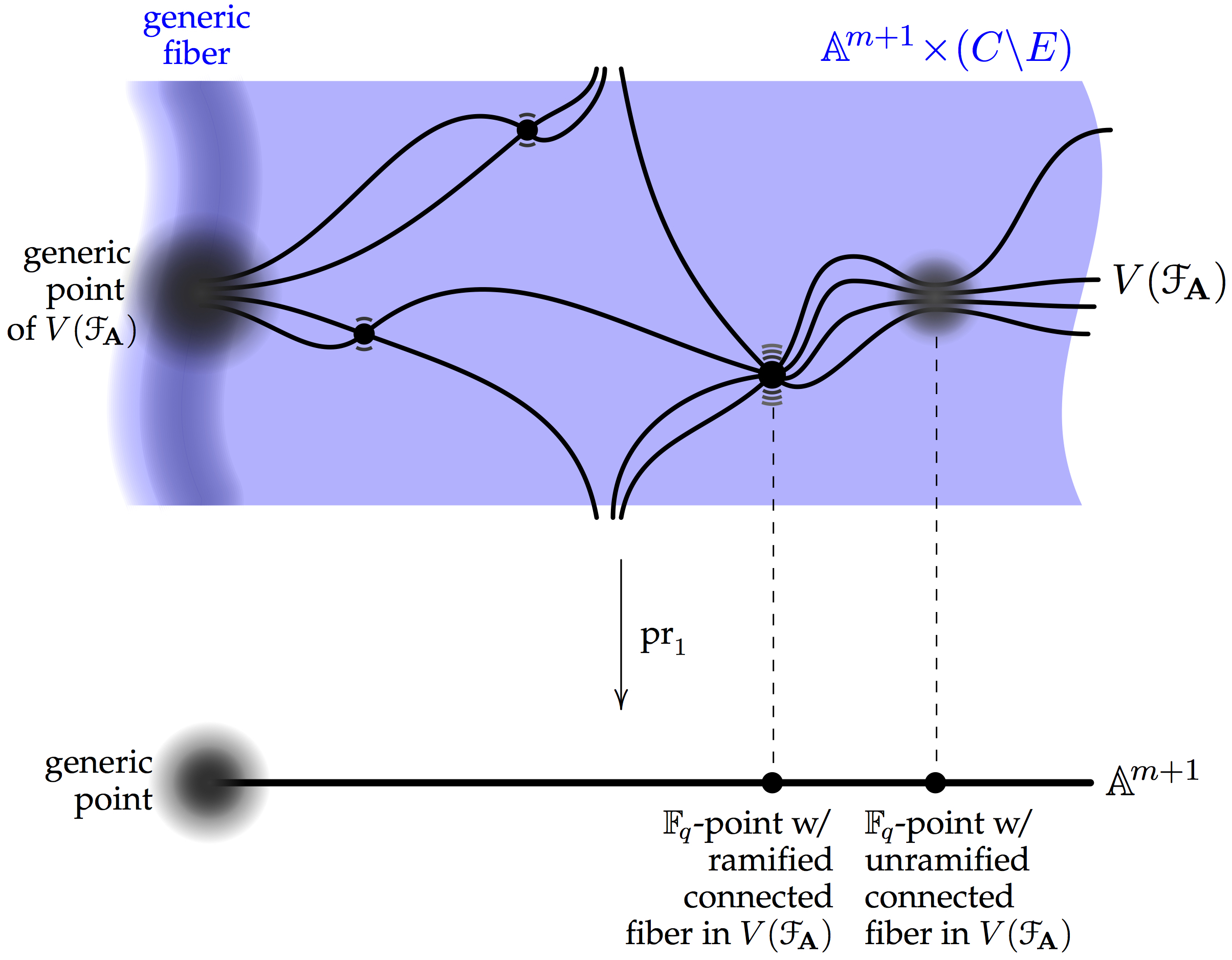 Figure 1
Peer Reviews
No public reviews on file for this paper yet. If you reviewed it on a platform where reviews are public (OpenReview, ICLR, NeurIPS, ICML), you can paste yours below so the community can read it here.
Videos
No videos yet. Explain this paper in a talk, walkthrough, or lecture? Add one.
Primes in short intervals on curves over finite fields
Efrat Bank
Efrat Bank
University of Michigan Mathematics Department
530 Church Street
Ann Arbor, MI 48109-1043
United States
and
Tyler Foster
Tyler Foster
Max Planck Institute for Mathematics
Vivatsgasse 7
53111 Bonn
Germany
Abstract.
We prove an analogue of the Prime Number Theorem for short intervals on a smooth projective geometrically irreducible curve of arbitrary genus over a finite field. A short interval “of size ” in this setting is any additive translate of the space of global sections of a sufficiently positive divisor by a suitable rational function . Our main theorem gives an asymptotic count of irreducible elements in short intervals on a curve in the “large ” limit, uniformly in and . This result provides a function field analogue of an unresolved short interval conjecture over number fields, and extends a theorem of Bary-Soroker, Rosenzweig, and the first author, which can be understood as an instance of our result for the special case of a divisor supported at a single rational point on the projective line.
Contents
- 1 Introduction
- 2 Short intervals on curves
- 3 Galois group of a generic element in a short interval
- 4 Calculation of the Galois group
- 5 Proof of Theorem A
1. Introduction
In this paper, we give an asymptotic count of irreducible elements inside short intervals on a smooth projective geometrically irreducible curve over a finite field. Our main result (§1.3, Theorem A) provides a function field analogue of an unresolved short interval conjecture for number fields (Conjecture 1.3.1), and extends a short interval theorem of Bary-Soroker, Rosenzweig, and the first author [2, Corollary 2.4] for polynomials over finite fields.
The notion of short intervals on a curve which we use is a natural analogue of the familiar notion of short intervals over the integers. In this introduction, we review what is known about short intervals over the integers, over number fields, and over polynomials with coefficients in a finite field. The analogies that run between these different settings lead naturally to our definition of a short interval on a curve and to the statement of our main result.
1.1. The Prime Number Theorem for short intervals
The Prime Number Theorem (PNT) states that the asymptotic density of prime integers in real intervals is . In other words, if we let denote the prime counting function
[TABLE]
then
[TABLE]
We get more refined statements by considering the asymptotic density of primes in families of smaller intervals. Letting be a real valued function with , we can ask for the density of primes in the intervals I(x,\Phi)\operatorname{\overset{{}_{\text{def}}}{=}}\big{[}x-\Phi(x),x+\Phi(x)\big{]} as . Define
[TABLE]
Then the naive conjecture on the asymptotic density of primes in the intervals is
[TABLE]
For fixed and , it is a straightforward consequence of the PNT that (2) holds. Assuming the Riemann hypothesis, (2) holds for \Phi(x)=x^{\varepsilon+\mbox{{\smaller\smaller\smaller\smaller\smaller\frac{1}{2}}}} for small . On the other hand, Maier [22] established what is now known as the “Maier phenomenon”: for , with , the asymptotic formula (2) fails. A classical conjecture predicts the following “short interval” prime number conjecture:
Conjecture 1.1.1**.**
For and , the asymptotic formula (2) holds.
In its full generality, Conjecture 1.1.1 is still open. Heath-Brown [15], improving on Huxley [16], proved Conjecture 1.1.1 for . We refer the reader to the surveys of Granville [7, 8] for additional background.
1.2. The Prime Polynomial Theorem for short intervals over
For each finite field , the analogy between number fields and function fields provides us with the following table of corresponding sets and quantities:
[TABLE]
If we let denote the prime polynomial counting function
[TABLE]
then, in accord with Table (3), the Prime Polynomial Theorem (PPT) asserts that
[TABLE]
Table (3) also suggests a natural definition of short intervals in :
Definition 1.2.1**.**
Given any monic non-constant polynomial and any positive real number , the corresponding interval (around ) is the set
[TABLE]
If and denotes the space of polynomials of degree at most , then . We say that is a short interval if , i.e., if .
Remark 1.2.2**.**
Note that in view of Definition 1.2.1, the set of monic polynomials of degree is the short interval .
Initial results on the density of prime polynomials in short intervals can be deduced from the work of Cohen [4] when , and from the work of Keating and Rudnick [18] in an almost everywhere sense. In [2], the first author together with Bary-Soroker and Rosenzweig prove the following analogue of Conjecture 1.1.1 in the large limit:
Theorem 1.2.3**.**
[2, Corollary 2.4]****. For fixed and a monic polynomial satisfying and , define
[TABLE]
Then the asymptotic formula
[TABLE]
holds uniformly for all monic of degree and all
[TABLE]
1.3. Short interval conjectures over number fields
One can extend Conjecture 1.1.1 to arbitrary number fields. However, because the relevant notions in have several competing generalizations to number fields larger than , there are several competing generalizations of Conjecture 1.1.1. If we let be an algebraic number field of degree over , with ring of integers , then each prime comes with a norm . The norm of an element is by definition the norm of the ideal that generates. We have both a prime ideal and a principal prime ideal counting function:
[TABLE]
Landau’s Prime Ideal Theorem (PIT) [20] states that
[TABLE]
Letting denote the class number of , the Principal PIT [25, §7.2, Corollary 4] states that
[TABLE]
As before, we can attempt to refine these density theorems by considering any real valued function , with , the corresponding (real) intervals and the prime ideal counting function
[TABLE]
The naive guess about the asymptotic behavior of \pi_{K}\big{(}I(x,\Phi)\big{)} is that
[TABLE]
When for fixed , formula (9) follows directly from the PIT. Balog and Ono [1], using formulas for the prime ideal counting function due to Lagarias and Odlyzko [19] and zero density estimates for Dedekind zeta-functions due to Heath-Brown [14] and Mitsui [24], show that formula (9) holds for x^{1-\mbox{{\smaller\smaller\smaller\smaller\frac{1}{c}}}+\varepsilon}\leq\Phi(x)\leq x. Here one may take if , and one can take if the degree of the extension is at least . Assuming the Riemann Hypothesis for the Dedekind zeta function , Grenié, Molteni, and Perelli [9] show that (9) holds for all \Phi(x)=\big{(}n\log x+\log|\text{disc}(K)|\big{)}\sqrt{x}.
In a general number field, the norm of an element is not equal to the absolute value of at a single infinite place of . Likewise, given an element with , and given , the set of all satisfying \big{|}N_{K}(a)-x\big{|}\leq x^{\varepsilon} (with the absolute value in ) is not necessarily the same as the set of all satisfying . This ambiguity in generalizing the basic quantities in Conjecture 1.1.1 gives us at least two distinct conjectures that can be seen as extensions Conjecture 1.1.1 to an arbitrary number field :
Conjecture 1.3.1**.**
Let . There exists some constant such that for each real vector in , the count
[TABLE]
satisfies the asymptotic formula
[TABLE]
Conjecture 1.3.2**.**
There exists some constant such that for each , the count
[TABLE]
satisfies the asymptotic formula
[TABLE]
Remark 1.3.3**.**
For , Conjectures 1.3.1 and 1.3.2 both recover Conjecture 1.1.1 if .
1.4. Main result: short intervals on arbitrary curves over
Let be a smooth projective geometrically irreducible curve over . As shown in [27, Theorem 5.12], the natural analogue of the PNT holds on , which is to say that the counting function
[TABLE]
satisfies the asymptotic formula
[TABLE]
One can formulate analogues of each of the Conjectures 1.3.1 and 1.3.2 on . In the present paper, we focus our attention to the analogue of Conjecture 1.3.1 in the large limit. We intend to address analogues of Conjecture 1.3.2 in a future paper.
On , the natural analogue of the “short interval” implicit in Conjecture 1.3.1 is the following set:
Definition 1.4.1**.**
Let be an effective divisor on , and let be a regular function on the complement of . The interval (of size around ) is the set
[TABLE]
where H^{0}\big{(}C,\mathscr{O}(E)\big{)} is the space of regular functions on with a pole of order at most at each point , for .
The interval is a short interval if the order of the pole of at each is strictly greater than .
Remark 1.4.2**.**
When and , for , Definitions 1.4.1 and 1.2.1 coincide.
The value that serves as our prime count in any short interval is
[TABLE]
The central result of the present paper is the following theorem, which establishes a function field analogue of Conjecture 1.1.1 and its generalization 1.3.1. In addition, this result extends Theorem 1.2.3 to curves of arbitrary genus over :
Theorem A**.**
Let be a smooth projective geometrically irreducible curve of genus over . Fix a positive integer . Let be an effective divisor on , and let be a regular function on such that the sum of the orders of all poles of is equal to , and such that is a short interval. Assume that either
- (i)
for some effective divisor with , or
- (ii)
, for some effective divisor with , such that the differential vanishes on a nonempty finite subset of .
Then
[TABLE]
where the implied constant in the error term depends only on and .
Remark 1.4.3**.**
To establish Theorem A, we prove a result (Theorem 5.2.1) that is stronger than Theorem A. For any partition type of the set , we provide an asymptotic count of rational functions whose associated principal divisor on has that partition type.
Remark 1.4.4**.**
Note that since is a short interval, all poles of lie in , and for each , the order of each pole of at is strictly greater than the order of at . Because is the sum of orders of all poles of , Definition 1.4.1 then implies that is equal to the sum .
1.5. Outline of the paper
In broad outline, our strategy for proving Theorem A is similar to the strategy taken in [2]; the key insight of the present paper is that specific positivity hypotheses for divisors on allow one to adapt the steps of the original argument in [2, §3 and §4] to a curve of arbitrary genus. In more detail, the outline of the paper is as follows.
In §2 we review the divisor theory and positivity conditions we will need. We introduce a variety parameterizing the elements of a short interval, and we use this variety to describe the generic element in a short interval. In §3 we explain how to associate a Galois group to the generic element. Most of the work in this section lies in showing that the Galois group is well defined. In §4 we calculate the Galois group. Specifically, we show that it is isomorphic to a symmetric group by verifying the conditions in a particular characterization of the symmetric group. In §5 we use our knowledge of this Galois group, along with some basic facts about étale morphisms, to show that a key counting result in [2], originally stated only for the genus zero case, can be extended to a count in any genus. Finally, we use this count to prove Theorem A and its stronger form Theorem 5.2.1. Our arguments in §5 make crucial use of the Lang-Weil estimates [21] and Bary-Soroker’s Chebotarev-type result [3, Proposition 2.2].
1.6. Acknowledgments
The authors would like to thank Lior Bary-Soroker and Michael Zieve for many conversations during our work on this paper that were crucial to its success. We also extend a warm thank you to Jeff Lagarias for comments on a draft of the paper and for his assistance in formulating prime density theorems in number fields. The exposition benefited greatly from an invitation to speak at the Palmetto Number Theory Series, held at the University of South Carolina and organized by Matthew Boylan, Michael Filaseta, and Frank Thorne, and from an invitation by Jordan Ellenberg to speak in the Number Theory Seminar at the University of Wisconsin–Madison.
We are especially thankful to Brian Conrad for looking closely at an earlier version of this paper, for pointing out a gap in our uniformity argument (now filled), for pointing out that we needed to prove what is now Proposition 3.3.6, and for suggesting that we use [5, §1, Lemma 1.5] to do so.
The authors conducted the research that lead to this paper while at the University of Michigan and while the second author was a visiting researcher at L’Institut des Hautes Études Scientifiques, at L’Institut Henri Poincaré, and at the Max Planck Institute for Mathematics. We thank all four institutions for their hospitality. The first author was partially supported by Michael Zieve’s NSF grant DMS-1162181. Support for the second author came from NSF RTG grant DMS-0943832 and from Le Laboratoire d’Excellence CARMIN.
2. Short intervals on curves
Fix a finite field , an algebraic closure \overline{{\mathbb{F}}_{\!q}}\big{/}{\mathbb{F}}_{\!q}, and a smooth projective geometrically irreducible curve over of arithmetic genus .
2.1. Divisors on a curve
We make extensive use of the theory of divisors on algebraic varieties (see [13, §II.6] for instance). We briefly review the most pertinent aspects of the theory.
By a divisor on , we mean a Weil divisor on . We denote the support of a divisor by , although we drop the distinction between and its support when it will not lead to confusion. For instance, we write instead of . If is a rational function on , we denote its associated principal divisor by . Given a divisor on , its divisor of zeros and divisor of poles are, respectively, the effective divisors
[TABLE]
Note that .
Each divisor on determines a sheaf of rational functions on whose value at each open subset is
[TABLE]
For each , the -vector space H^{i}\big{(}C,\mathscr{O}(D)\big{)} is finite dimensional. We stress that according to the definition of that we use, the space of global sections H^{0}\big{(}C,\mathscr{O}(D)\big{)} is canonically a space of rational functions on .
For each , fix homogeneous coordinates on . Let denote the hyperplane cut out by . If H^{0}\big{(}C,\mathscr{O}(D)\big{)} admits a basis such that at least one of the functions is non-vanishing at each , we say that is basepoint free. If is basepoint free, then our basis gives rise to a morphism
[TABLE]
into projective space of dimension
[TABLE]
The divisor is very ample if is basepoint free and the morphism (15) is a closed embedding. Every divisor on satisfying is very ample.
If is an effective very ample divisor on , then the basis of H^{0}\big{(}C,\mathscr{O}(E)\big{)} can be chosen so that , with
[TABLE]
In particular, if is an effective very ample divisor, then the open subscheme is affine, and its ring of regular functions is generated by the coordinates on . We consistently use the notation
[TABLE]
Remark 2.1.1**.**
Note that if and are divisors on satisfying , then we have a natural inclusion H^{0}\big{(}C,\mathscr{O}(D_{0})\big{)}\subset H^{0}\big{(}C,\mathscr{O}(D)\big{)}. Thus if is very ample and , then is also very ample.
Remark 2.1.2**.**
Given a field extension , each point in has a unique factorization locally on . The pullback of to is the divisor
[TABLE]
Note that , and that if is effective, then is effective as well. The sheaf on pulls back to a sheaf on , and we have a canonical isomorphism [12, §9.4.2], thus is very ample whenever is.
2.2. Generic element in a short interval
Let be an effective very ample divisor on . Then following Definition 1.4.1, each regular function on determines an interval
[TABLE]
The fact that and H^{0}\big{(}C,\mathscr{O}(E)\big{)}\subset R implies that .
Choose a basis of H^{0}\big{(}C,\mathscr{O}(E)\big{)} as in §16. Then we have a corresponding interpretation of
[TABLE]
as a variety parameterizing the functions in . Let denote the field of rational functions , and define
[TABLE]
On the trivial family of curves , we have a regular function
[TABLE]
See Figure 1 for a depiction of the scheme cut out by inside the family . The restriction of to the generic fiber of this trivial family describes the generic element of . If we denote -rational points in as -tuples , then for each , the restriction of (17) to the fiber is an element of . The value \pi_{C}\big{(}I(f,E)\big{)} becomes the count of a particular set of -rational points in :
[TABLE]
3. Galois group of a generic element in a short interval
For any field and any irreducible separable polynomial , the residue field admits a unique splitting field inside any separable closure . When we interpret as the field obtained by adjoining a single root of to , it becomes natural to construct as the field obtained by adjoining all roots of to . We can also construct without any explicit reference to roots of . Indeed, is the normal closure of inside [26, Theorem 2.9.5.(4)]. This latter characterization of the splitting field generalizes to the higher genus setting and, as we demonstrate in the present section, allows us to define the Galois group of the generic element in short intervals on .
3.1. The setting of §3 and §4
The following datum is to remain fixed throughout §3 and §4: Let be an effective very ample divisor on , define to be the ring of regular functions on the affine curve , and let be a regular function on satisfying
[TABLE]
where denotes the coefficient of in . Define
[TABLE]
Note that the inequality (19) and the quantity are unaffected by base change along any field extension . Let be the short interval defined by and . Let be the generic element in as defined in (17). Fix an algebraic closure such that .
Remark 3.1.1**.**
In the case where and is an effective divisor on supported at , we have H^{0}\big{(}\mathbb{P}^{1},\mathscr{O}(E)\big{)}={\mathbb{F}}_{\!q}[t]^{\leq m}, where . The choice of a regular function amounts to the choice of a polynomial , and k=\text{deg}\big{(}\text{div}(f)_{-}\big{)}=\text{deg}_{\ \!}f. Thus the inequality (19) reduces to the requirement that appears in the form “” in Theorem 1.2.3.
Remark 3.1.2**.**
In §5, where we consider the asymptotic behavior of , we will allow and to vary subject to the constraint (19).
3.2. The splitting field and Galois group of a relative separable point
We can associate Galois groups to a large class of points in as follows:
Definition 3.2.1**.**
Let be an algebraic extension. For a prime ideal in the ring , denote by the residue field of . The splitting field of (over ), denoted or , is the normal closure of in .
If the extension is separable, then the Galois group of is
[TABLE]
Remark 3.2.2**.**
For a prime ideal in , the fact that is separable is equivalent to the statement that
[TABLE]
(see [30, Proposition 5.3.9, Definition 5.3.12 and Proposition 5.3.16.(1)]). Since is a Dedekind domain, the isomorphism (20) is equivalent to the statement that in the ring , the ideal has prime factorization
[TABLE]
where and for each . The Galois group acts faithfully and transitively on the prime factors .
3.3. Primality and separability of the generic element
For any field extension , define
[TABLE]
The canonical morphism lets us interpret both and as elements of . By §2.1 and [10, Corollaire 6.9.9], we have
[TABLE]
and becomes a variety parameterizing elements in .
Lemma 3.3.1**.**
For any field extension , the ideal generated by is prime in .
Proof.
Let be the variety cut out by in {\mathbb{A}}^{\!m+1}\times\big{(}C_{K}\!\smallsetminus\!E_{K}\big{)} . The projections
[TABLE]
restrict to morphisms
[TABLE]
Assume that is not prime. Then either the morphism has empty generic fiber, or else the subscheme V(\mathcal{F}_{\!\mathbf{A}})\subset{\mathbb{A}}^{\!m+1}_{K}\!\times\!\big{(}C_{K}\!\smallsetminus\!E_{K}\big{)} has more than one irreducible component.
Comparing the strict inequalities (19) with the inequality defining the inclusion
[TABLE]
we see that for all . Thus
[TABLE]
In particular, is not a unit in , and does not have empty generic fiber.
Because is pure of codimension- inside {\mathbb{A}}^{\!m+1}\!\times\big{(}C_{K}\!\smallsetminus\!E_{K}\big{)}, whereas is -dimensional, an irreducible component of is either a whole fiber of the projection in (22) over a closed point of , or else its generic point lies over the generic point of . For any point , the function is linear in the variables , and is nonzero since has coefficient . For closed points , this shows that closed fibers of the morphism in (22) cannot be irreducible components of . Over the generic point of , linearity of the nonzero function implies that the ideal is prime. Thus has a unique irreducible component. ∎
Remark 3.3.2**.**
Since is a curve, Lemma 3.3.1 implies that the subscheme consists of a single closed point . The residue field \kappa(\mathfrak{P}_{K})=R_{K}(\mathbf{A})\big{/}(\mathcal{F}_{\!\mathbf{A}}) is a finite extension of .
Lemma 3.3.3**.**
For any field extension , the extension \kappa(\mathfrak{P}_{K})\big{/}K(\mathbf{A}) in Remark 3.3.2 is separable.
Proof.
For each homogenous function on , let denote the distinguished open subscheme of where is nonzero. The fact that is very ample allows us to choose a polynomial such that the regular function is the restriction of to . The function on is then the restriction of the function
[TABLE]
The curve is smooth, therefore there exist functions and for which the point in Remark 3.3.2 lies in the affine open neighborhood
[TABLE]
and such that the determinant of the -minor in the matrix
[TABLE]
is invertible on . The entries in the last row of all have the explicit form
[TABLE]
Hence, the term associated to in the cofactor expansion of is the only cofactor term in which appears. The coefficient of in this term is nonzero at , therefore is nonzero at . The -scheme is then smooth of relative dimension [math] over , or equivalently, is étale over [23, §I.3, Corollary 3.16], and the field extension is separable [23, §I.3, Proposition 3.2.(a) & (e)]. ∎
From Lemmas 3.3.1 and 3.3.3, we immediately have the following:
Corollary 3.3.4**.**
For each algebraic extension , the prime ideal has an associated Galois group, which we henceforth denote
\text{Gal}\big{(}\mathcal{F}_{\!\mathbf{A}},K(\mathbf{A})\big{)}\ \ \operatorname{\overset{{}_{\text{def}}}{=}}\ \ \text{Gal}\big{(}\mathfrak{P}\big{/}K(\mathbf{A})\big{)}.
Lemma 3.3.5**.**
For each algebraic field extension , there is an inclusion of Galois groups
[TABLE]
Proof.
Since is isomorphic to the compositum , we have isomorphisms
[TABLE]
Post-composing (26) with the inclusion \text{Gal}\big{(}\kappa(\mathfrak{P}_{K})\big{/}K(\mathbf{A})\big{)}\hookrightarrow\text{Gal}\big{(}\kappa(\mathfrak{P}_{K})\big{/}{\mathbb{F}}_{\!q}(\mathbf{A})\big{)}, we obtain the embedding (25). ∎
Proposition 3.3.6**.**
The branch locus of the morphism has codimension in , and its compliment is the maximal open subset of over which is finite étale.
Proof.
Lemma 3.3.3 implies that is generically unramified over , and thus that has codimension in . Define
[TABLE]
Then the resulting morphism is finite, surjective, and unramified of degree . The variety is a normal, and surjectivity of implies that for each , the morphism of stalks is injective [29, Tag 0CC1, (1) & (6)]. Thus by [5, §1, Lemma 1.5], the morphism is étale. Because is the branch locus , this implies that is the maximal open subset of over which is finite étale. ∎
4. Calculation of the Galois group
4.1. A characterization of the symmetric group
Recall from §3.1 that we fix an effective very ample divisor on and a function regular on with poles satisfying the inequalities (19), and that . Let denote the symmetric group on letters. Our goal in the present section is to prove the following:
Theorem 4.1.1**.**
Assume that satisfies one of the following two conditions
- (a)
There exists a very ample effective divisor on such that ;
- (b)
There exists a very ample effective divisor on such that , , and vanishes on a finite nonempty set.
Then the Galois group \text{Gal}\big{(}\mathcal{F}_{\!\mathbf{A}},{\mathbb{F}}_{\!q}(\mathbf{A})\big{)} is isomorphic to .
Remark 4.1.2**.**
To prove Theorem 4.1.1, we use the following characterization of :
Lemma 4.1.3**.**
[28, Lemma 4.4.3]****. A subgroup is equal to if and only if satisfies the following three conditions:
- (i)
is transitive;
- (ii)
is doubly transitive;
- (iii)
contains a transposition.
Beginning of the proof of Theorem 4.1.1. Observe that for any algebraic extension the condition (19) and its consequence (23), combined with the fact that the total degree of any principal divisor is [math], imply that . Thus by Remark 3.2.2, the Galois group \text{Gal}\big{(}\mathcal{F}_{\!\mathbf{A}},K(\mathbf{A})\big{)} comes with a natural faithful action on a set of elements, namely the prime factors in (21). In this way, we obtain an embedding
[TABLE]
for each algebraic extension . For the special case , Lemma 3.3.5 tells us that the inclusion (27) factors as
[TABLE]
It therefore suffices to check that the Galois group \text{Gal}\big{(}\mathcal{F}_{\!\mathbf{A}},\overline{{\mathbb{F}}_{\!q}}(\mathbf{A})\big{)} satisfies the three conditions in Lemma 4.1.3. We verify these conditions in §4.2 and §4.3 below.
4.2. Transitivity and double transitivity
By Remark 3.2.2, the embedding (27) realizes the group \text{Gal}\big{(}\mathcal{F}_{\!\mathbf{A}}\big{/}\overline{{\mathbb{F}}_{\!q}}(\mathbf{A})\big{)} as a transitive subgroup of . Varifying condition (ii) of Lemma 4.1.3 in the setting of Theorem 4.1.1 amounts to proving the following:
Proposition 4.2.1**.**
If satisfies either of the conditions (a) or (b) in Theorem 4.1.1, then the subgroup \text{Gal}\big{(}\mathcal{F}_{\!\mathbf{A}}\big{/}\overline{{\mathbb{F}}_{\!q}}(\mathbf{A})\big{)}\subset S_{k} is doubly transitive.
Remark 4.2.2**.**
Note that each of the conditions (a) and (b) of Theorem 4.1.1 imply the following weaker condition: for any degree- point in the support of , the divisor is again effective and very ample.
Proof of Proposition 4.2.1..
Because \text{Gal}\big{(}\mathcal{F}_{\!\mathbf{A}}\big{/}\overline{{\mathbb{F}}_{\!q}}(\mathbf{A})\big{)} is transitive, it is enough to show that there exists a factor in (21) for which the stabilizer subgroup of inside \text{Gal}\big{(}\mathcal{F}_{\!\mathbf{A}}\big{/}\overline{{\mathbb{F}}_{\!q}}(\mathbf{A})\big{)} is transitive on the set of factors .
Fix a single -valued point \mathfrak{q}\in V(f)\subset C_{\mbox{{\smaller\smaller\smaller\smaller\smaller\overline{{\mathbb{F}}{!q}!}}}}\!\smallsetminus\!E_{\mbox{{\smaller\smaller\smaller\smaller\smaller\overline{{\mathbb{F}}{!q}!}}}}. Choose a hyperplane L\subset\mathbb{P}^{m}_{\mbox{{\smaller\smaller\smaller\smaller\smaller\overline{{\mathbb{F}}{!q}!}}}} such that the only point of in C_{\mbox{{\smaller\smaller\smaller\smaller\smaller\overline{{\mathbb{F}}{!q}!}}}}\cap L is . Define to be the effective divisor associated to the weighted intersection C_{\mbox{{\smaller\smaller\smaller\smaller\smaller\overline{{\mathbb{F}}{!q}!}}}}\cap L. Choose a linear form satisfying E^{\prime}=\text{div}(\ell)+E_{\mbox{{\smaller\smaller\smaller\smaller\smaller\overline{{\mathbb{F}}{!q}!}}}}, and let \mathfrak{h}\in{\mathbb{A}}^{\!m+1}_{\mbox{{\smaller\smaller\smaller\smaller\smaller\overline{{\mathbb{F}}_{!q}!}}}} be the generic point of the hyperplane cut out by the equation . Let denote the restriction of to . Then factors as
[TABLE]
where is a basis of the subspace of H^{0}\big{(}C_{\mbox{{\smaller\smaller\smaller\smaller\smaller\overline{{\mathbb{F}}{!q}!}}}},\mathscr{O}(E_{\mbox{{\smaller\smaller\smaller\smaller\smaller\overline{{\mathbb{F}}{!q}!}}}})\big{)} corresponding the hyperplane V(\mathfrak{h})\subset{\mathbb{A}}^{\!m+1}_{\mbox{{\smaller\smaller\smaller\smaller\smaller\overline{{\mathbb{F}}{!q}!}}}}, and where is a regular function on C_{\mbox{{\smaller\smaller\smaller\smaller\smaller\overline{{\mathbb{F}}{!q}!}}}}\!\smallsetminus\!(E^{\prime}-\mathfrak{q}) satisfying
[TABLE]
The linear equivalence E^{\prime}\sim E_{\mbox{{\smaller\smaller\smaller\smaller\smaller\overline{{\mathbb{F}}{!q}!}}}} makes very ample, thus \text{dim}_{\ \!}H^{0}\big{(}C_{\mbox{{\smaller\smaller\smaller\smaller\smaller\overline{{\mathbb{F}}{!q}!}}}},\mathscr{O}(E^{\prime}-\mathfrak{q})\big{)}=m with basis . This implies that the linear combination
[TABLE]
is the generic element of the interval . By Remark 4.2.2, is effective and very ample. Hence (28) and Lemmas 3.3.1 and 3.3.3 provide us with a Galois group \text{Gal}\big{(}\mathcal{F}_{\!\mathbf{A}^{\prime}},\overline{{\mathbb{F}}_{\!q}}(\mathbf{A}^{\prime})\big{)}.
Let denote the coordinate ring of the affine curve C_{\mbox{{\smaller\smaller\smaller\smaller\smaller\overline{{\mathbb{F}}{!q}!}}}}\!\smallsetminus\!E^{\prime}. Observe that since , the inequalities (19) imply that \mathfrak{P}_{\mbox{{\smaller\smaller\smaller\smaller\smaller\overline{{\mathbb{F}}{!q}!}}}} lies in C_{\mbox{{\smaller\smaller\smaller\smaller\smaller\overline{{\mathbb{F}}{!q}!}}}(\mathbf{A})}\!\smallsetminus\!E^{\prime}_{\mbox{{\smaller\smaller\smaller\smaller\smaller\overline{{\mathbb{F}}{!q}!}}}(\mathbf{A})}. Consider the point inside . Because Lemma 3.3.3 says that is separable, whereas is a codimension- point in {\mathbb{A}}^{\!m+1}_{\mbox{{\smaller\smaller\smaller\smaller\smaller\overline{{\mathbb{F}}{!q}!}}}}, the point corresponds to a discrete valuation on \kappa(\mathfrak{P}_{\mbox{{\smaller\smaller\smaller\smaller\smaller\overline{{\mathbb{F}}{!q}!}}}}). Thus the Galois group \text{Gal}\big{(}\text{split}(\mathfrak{P}_{\mbox{{\smaller\smaller\smaller\smaller\smaller\overline{{\mathbb{F}}{!q}!}}}})\big{/}\kappa(\mathfrak{P}_{\mbox{{\smaller\smaller\smaller\smaller\smaller\overline{{\mathbb{F}}{!q}!}}}})\big{)} acts transitively on the roots of any monic polynomial whose roots generate the extension \text{split}(\mathfrak{P}^{\prime})\big{/}\kappa(\mathfrak{P}^{\prime}). Because \text{Gal}\big{(}\text{split}(\mathfrak{P}_{\mbox{{\smaller\smaller\smaller\smaller\smaller\overline{{\mathbb{F}}{!q}!}}}})\big{/}\kappa(\mathfrak{P}_{\mbox{{\smaller\smaller\smaller\smaller\smaller\overline{{\mathbb{F}}{!q}!}}}})\big{)} is a subgroup of \text{Gal}\big{(}\mathcal{F}_{\!\mathbf{A}},\overline{{\mathbb{F}}_{\!q}}(\mathbf{A})\big{)}, this completes the proof. ∎
4.3. Presence of a transposition
Fix an algebraic closure , and define to be the algebraic closure inside .
Consider the morphism . It restricts to the morphism of affine schemes
[TABLE]
dual to the morphism of -algebras that takes . Since is effective and very ample, we can choose a lift of as in the proof of Lemma 3.3.3, and (29) becomes the restriction of the morphism
[TABLE]
which takes
[TABLE]
Proposition 4.3.1**.**
At each point in , the ramification order of is at most .
Proof.
Let denote the -module of Kähler differentials on , and let denote the Kähler differential of . In , on a sufficiently small affine open neighborhood of each point , we have a matrix as in equation (24), where the regular functions cut out U_{\mathbf{x}}\cup\big{(}C_{L}\!\smallsetminus\!E_{L}\big{)}. Since , the ramification divisor of is the effective divisor corresponding to the subscheme V\big{(}\text{det}(M)\big{)}\cap\big{(}C_{L}\!\smallsetminus\!E_{L}\big{)} inside . The points of U_{\mathbf{x}}\cap\big{(}C_{L}\!\smallsetminus\!E_{L}\big{)} where has ramification order are exactly the reduced points of V\big{(}\text{det}(M)\big{)}\cap\big{(}C_{L}\!\smallsetminus\!E_{L}\big{)}. Thus is suffices to prove that the -scheme V\big{(}\text{det}(M)\big{)}\cap\big{(}C_{L}\!\smallsetminus\!E_{L}\big{)} is smooth.
For each , let denote the minor of that we obtain by removing the -row and -column of , so that
[TABLE]
From the proof of Lemma 3.3.3, we know that is nonzero everywhere on U_{\mathbf{x}}\cap\big{(}C_{L}\!\smallsetminus\!E_{L}\big{)}. Therefore is invertible on some open neighborhood of U_{\mathbf{x}}\cap\big{(}C_{L}\!\smallsetminus\!E_{L}\big{)} inside . In this neighborhood, the vanishing locus of coincides with V\big{(}\text{det}(M)\big{)}. Write
[TABLE]
where is a regular function with no dependence. Then V\big{(}\text{det}(M)\big{)} is singular at precisely those points where the determinant of the -matrix
[TABLE]
vanishes. The absence of from means that the zeros of are defined over the subfield , whereas the zeros of (30) are defined over the subfield . Because zeros of (30) are not -rational, this completes the proof. ∎
Proposition 4.3.2**.**
The morphism is ramified at some point in in each of the following two cases:
- (i)
;
- (ii)
.
Proof.
The rational function on determines a morphism . By definition, and differ by the constant , and so it suffices to show that is ramified at some point of .
At each point , let denote the ramification order of at (the order of vanishing of the Kähler differential at ). Define
[TABLE]
Then . Recall that k=\text{deg}\big{(}\text{div}(f)_{-}\big{)}. Lemmas 3.3.1 and 3.3.3 imply that the morphism is finite and separable, so satisfies Riemann-Hurwitz [13, §IV, Corollary 2.4]. Since is the degree of , this gives
[TABLE]
Thus it suffices to show that
[TABLE]
Fix a point , and fix a uniformizing parameter in the stalk . Let denote the order of at , and recall that denotes the degree of the pole of at . Because is effective, our assumption (19) implies that . Because is very ample, H^{0}\big{(}C_{L},\mathscr{O}(E_{L})\big{)} is basepoint free, and thus there exists some nontrivial -linear combination of the variables so that we can write the rational function on as
[TABLE]
where the order of the pole of \mathcal{G}_{\mathbf{A}}\big{(}\frac{1}{z}\big{)} at is between 1 and . Write
[TABLE]
where is an -rational function that does not vanish at , and where the order of vanishing of at is between and . Thus the order of vanishing of d\big{(}\frac{1}{\mathcal{F}_{\!\mathbf{A}}}\big{)} at is equal to the order of vanishing of the function
[TABLE]
at . This implies that:
If does not divide , then ;
If divides , then .
Repeating this argument at all points in , we see that
[TABLE]
Thus (31) is satisfied whenever or . ∎
Proposition 4.3.3**.**
Assume that one of the following two conditions holds:
- (a)
There exists a very ample effective divisor on such that ;
- (b)
There exists a very ample effective divisor on such that , , and vanishes at a nonempty finite set.
Then the morphism separates critical points in , i.e., there do not exist distinct points satisfying the system of equations
[TABLE]
Proof.
It suffices to prove that the morphism separates critical points. Assume that , with a very ample effective divisor on , and with or . Let m_{0}=\text{dim}_{\ \!}H^{0}\big{(}C,\mathscr{O}(E_{0})\big{)}-1. Interpret as a closed subvariety of via the closed embedding provided by . The standard proof of Bertini’s Theorem [13, §II.8, proof of Theorem 8.18] implies that for any two distinct points x,y\in C_{\mbox{{\smaller\smaller\smaller\smaller\smaller\overline{{\mathbb{F}}{!q}!}}}}\!\smallsetminus\!E_{\mbox{{\smaller\smaller\smaller\smaller\smaller\overline{{\mathbb{F}}{!q}!}}}}, we can choose a linear form on \mathbb{P}^{m_{0}}_{\mbox{{\smaller\smaller\smaller\smaller\smaller\overline{{\mathbb{F}}{!q}!}}}} whose restriction to C_{\mbox{{\smaller\smaller\smaller\smaller\smaller\overline{{\mathbb{F}}{!q}!}}}} provides local uniformizing parameters at and at . We can furthermore choose so that it satisfies the generic condition
[TABLE]
Since t\in H^{0}\big{(}C_{\mbox{{\smaller\smaller\smaller\smaller\smaller\overline{{\mathbb{F}}{!q}!}}}},\mathscr{O}(E_{0,\mbox{{\smaller\smaller\smaller\smaller\smaller\overline{{\mathbb{F}}{!q}!}}}})\big{)} and , we have 1,t,t^{2},\dots,t^{n}\in H^{0}\big{(}C_{\mbox{{\smaller\smaller\smaller\smaller\smaller\overline{{\mathbb{F}}{!q}!}}}},\mathscr{O}(E_{\mbox{{\smaller\smaller\smaller\smaller\smaller\overline{{\mathbb{F}}{!q}!}}}})\big{)}. Choose a new basis of H^{0}\big{(}C_{\mbox{{\smaller\smaller\smaller\smaller\smaller\overline{{\mathbb{F}}{!q}!}}}},\mathscr{O}(E_{\mbox{{\smaller\smaller\smaller\smaller\smaller\overline{{\mathbb{F}}{!q}!}}}})\big{)} such that for . Let denote linear generators of in this new basis, with . Then
[TABLE]
where . Define
[TABLE]
Again by the dimension counts in [13, §II.8, proof of Theorem 8.18], we can fix a Zariski open neighborhood U\subset C_{\mbox{{\smaller\smaller\smaller\smaller\smaller\overline{{\mathbb{F}}{!q}!}}}}\!\smallsetminus\!E_{\mbox{{\smaller\smaller\smaller\smaller\smaller\overline{{\mathbb{F}}{!q}!}}}} containing both and , such that the restriction of to C_{\mbox{{\smaller\smaller\smaller\smaller\smaller\overline{{\mathbb{F}}{!q}!}}}}\!\smallsetminus\!E_{\mbox{{\smaller\smaller\smaller\smaller\smaller\overline{{\mathbb{F}}{!q}!}}}} provides a uniformizing parameter at every point . Define
[TABLE]
At each -valued point in , the system of equations (32) holds for the function if and only if satisfies the single -valued matrix equation
[TABLE]
where denotes the regular function on such that as a global section of . Define functions on and on according to
[TABLE]
By (33), the -matrix at left in (35) has rank everywhere in . Hence (35) holds at if and only if satisfies the single determinant equation
[TABLE]
Interpret (36) as an equation over in the variables . Let T\subset{\mathbb{A}}^{\!m}_{\mbox{{\smaller\smaller\smaller\smaller\smaller\overline{{\mathbb{F}}{!q}!}}}}\times_{\mbox{{\smaller\smaller\smaller\smaller\smaller\overline{{\mathbb{F}}{!q}!}}}}U_{xy} denote the subscheme cut out by this equation, with projections
[TABLE]
Letting denote the generic point of {\mathbb{A}}^{\!m}_{\mbox{{\smaller\smaller\smaller\smaller\smaller\overline{{\mathbb{F}}_{!q}!}}}}, it suffices to prove that the fiber is empty. Because the leftmost matrix in (35) has rank , each fiber of in is at most -dimensional. The generic fiber of is cut out by a single equation in the -dimensional space . Thus if the determinant in (36) is not constantly equal to [math], we have
[TABLE]
which implies that the image \text{pr}_{1}(T)\subset{\mathbb{A}}^{\!m}_{\mbox{{\smaller\smaller\smaller\smaller\smaller\overline{{\mathbb{F}}{!q}!}}}} cannot contain the generic point of {\mathbb{A}}^{\!m}_{\mbox{{\smaller\smaller\smaller\smaller\smaller\overline{{\mathbb{F}}{!q}!}}}}. In order to show that (36) has no solutions in , it thus remains to show that the determinant appearing in (36) is not constantly equal to [math].
Let be the determinant that appears in (36). A straightforward calculation gives
[TABLE]
If , then the coefficient of in 2\ \!c(u,v)+\big{(}\ \!t(v)-t(u\ \!)\big{)}\ \!\big{(}\ \!\varphi(u)+\varphi(v)\ \!\big{)} is
[TABLE]
By (33), this last expression is nonzero in any characteristic. If and , then
[TABLE]
If is nonconstant in this case, then is not constantly zero.
Because the Zariski open subsets cover \big{(}C_{\mbox{{\smaller\smaller\smaller\smaller\smaller\overline{{\mathbb{F}}{!q}!}}}}\times C_{\mbox{{\smaller\smaller\smaller\smaller\smaller\overline{{\mathbb{F}}{!q}!}}}}\big{)}\!\smallsetminus\!\{\text{diagonal}\} as varies inside \big{(}C_{\mbox{{\smaller\smaller\smaller\smaller\smaller\overline{{\mathbb{F}}{!q}!}}}}\times C_{\mbox{{\smaller\smaller\smaller\smaller\smaller\overline{{\mathbb{F}}{!q}!}}}}\big{)}\!\smallsetminus\!\{\text{diagonal}\}, this completes the proof. ∎
Corollary 4.3.4**.**
Assume that one of the following two conditions holds:
- (a)
There exists a very ample effective divisor on such that ;
- (b)
There exists a very ample effective divisor on such that , , and vanishes on a nonempty finite set.
Then the subgroup \text{Gal}\big{(}\mathcal{F}_{\!\mathbf{A}}\big{/}\overline{{\mathbb{F}}_{\!q}}(\mathbf{A})\big{)}\subset S_{k} contains a transposition.
Proof.
If , then each of the conditions (a) and (b) implies condition (ii) of Proposition 4.3.2. Thus for any , the morphism is ramified at some closed point of . Let be such a point, which is to say that the morphism is ramified at . Proposition 4.3.1 says that the order of ramification at any point in is at most . Thus the factorization type of the fiber of containing is . As Proposition 4.3.3 says that the critical values of are distinct, this implies that has at least solutions. However, since is a ramification point, the fiber over has exactly one double point. Hence the inertia group over permutes two factors of and fixes all others. Thus \text{Gal}\big{(}\mathcal{F}_{\!\mathbf{A}}\big{/}\overline{{\mathbb{F}}_{\!q}}(\mathbf{A})\big{)} contains a transposition. ∎
Completion of the proof of Theorem 4.1.1..
By Remark 4.2.2, if either of the conditions (a) or (b) holds, then Proposition 4.2.1 holds and \text{Gal}\big{(}\mathcal{F}_{\!\mathbf{A}}\big{/}\overline{{\mathbb{F}}_{\!q}}(\mathbf{A})\big{)} is doubly transitive. By Corollary 4.3.4, \text{Gal}\big{(}\mathcal{F}_{\!\mathbf{A}}\big{/}\overline{{\mathbb{F}}_{\!q}}(\mathbf{A})\big{)} contains a transposition. By Lemma 4.1.3, we have \text{Gal}\big{(}\mathcal{F}_{\!\mathbf{A}}\big{/}\overline{{\mathbb{F}}_{\!q}}(\mathbf{A})\big{)}\cong S_{k}. ∎
5. Proof of Theorem A
We now use the Galois group calculation in §4 to prove Theorem A.
5.1. Setup for the proof of Theorem A
Let be the element defined in (17), and let denote the resulting projection. For each -rational point , let denote the restriction of to .
Proposition 5.1.1**.**
Let and be as in the statement of Theorem 4.1.1, and let denote the branch locus of . Then is pure of codimension in , and it satisfies the inequality
[TABLE]
where denotes the genus of .
Proof.
Define V\overset{{}_{\text{def}}}{=}H^{0}\big{(}C,\mathscr{O}\big{(}\text{div}(f)_{-}\big{)}\big{)}^{\ast}, the -vector space dual of the space of rational functions H^{0}\big{(}C,\mathscr{O}\big{(}\text{div}(f)_{-}\big{)}\big{)}, and consider the pair of dual projective spaces
[TABLE]
where and denote the graded symmetric -algebras on and , respectively. Because is a very ample effective divisor, the inequalities (19) imply that is very ample and effective. Identify with its image under the closed embedding
[TABLE]
induced by . Pass to the algebraic closure to obtain a smooth, closed, irreducible subvariety C_{\mbox{{\smaller\smaller\smaller\smaller\smaller\overline{{\mathbb{F}}{!q}!}}}}\subset\mathbb{P}(V_{\mbox{{\smaller\smaller\smaller\smaller\smaller\overline{{\mathbb{F}}{!q}!}}}}). By [17, §3.1.3 & §5.1], this subvariety determines a dual variety C^{\vee}_{\mbox{{\smaller\smaller\smaller\smaller\smaller\overline{{\mathbb{F}}{!q}!}}}}\ \subset\ \mathbb{P}(V^{\ast}_{\mbox{{\smaller\smaller\smaller\smaller\smaller\overline{{\mathbb{F}}{!q}!}}}}).
We claim that C^{\vee}_{\mbox{{\smaller\smaller\smaller\smaller\smaller\overline{{\mathbb{F}}{!q}!}}}} is a hypersurface in \mathbb{P}(V^{\ast}_{\mbox{{\smaller\smaller\smaller\smaller\smaller\overline{{\mathbb{F}}{!q}!}}}}). To see this, let denote the conormal sheaf on C_{\mbox{{\smaller\smaller\smaller\smaller\smaller\overline{{\mathbb{F}}{!q}!}}}} in , and let denote its associated projective scheme over C_{\mbox{{\smaller\smaller\smaller\smaller\smaller\overline{{\mathbb{F}}{!q}!}}}}, which comes with a projection
[TABLE]
(see [17, §3.1] for details). Note that \text{dim}_{\ \!}\mathbb{P}(\mathscr{N})=\text{dim}_{\ \!}\mathbb{P}(V_{\mbox{{\smaller\smaller\smaller\smaller\smaller\overline{{\mathbb{F}}{!q}!}}}})-1. By [17, Proposition 3.5], if the projection (39) is not everywhere ramified, then the projection (39) induces a birational morphism \mathbb{P}(\mathscr{N})\!\lx@xy@svg{\hbox{\raise 0.0pt\hbox{\kern 3.0pt\hbox{\ignorespaces\ignorespaces\ignorespaces\hbox{\vtop{\kern 0.0pt\offinterlineskip\halign{\entry@#!@&&\entry@@#!@\cr&\crcr}}}\ignorespaces{\hbox{\kern-3.0pt\raise 0.0pt\hbox{\hbox{\kern 0.0pt\raise 0.0pt\hbox{\hbox{\kern 3.0pt\raise 0.0pt\hbox{\textstyle{{}\ignorespaces\ignorespaces\ignorespaces\ignorespaces}}}}}}}}\ignorespaces\ignorespaces\ignorespaces{}\ignorespaces\ignorespaces{\hbox{\lx@xy@drawline@}}\ignorespaces{\hbox{\kern 27.0pt\raise 0.0pt\hbox{\hbox{\kern 0.0pt\raise 0.0pt\hbox{\lx@xy@tip{1}\lx@xy@tip{-1}}}}}}\ignorespaces\ignorespaces{\hbox{\lx@xy@drawline@}}\ignorespaces{\hbox{\lx@xy@drawline@}}{\hbox{\kern 27.0pt\raise 0.0pt\hbox{\hbox{\kern 0.0pt\raise 0.0pt\hbox{\hbox{\kern 3.0pt\raise 0.0pt\hbox{\textstyle{}}}}}}}}\ignorespaces}}}}\ignorespaces\!C^{\vee}_{\mbox{{\smaller\smaller\smaller\smaller\smaller\overline{{\mathbb{F}}{!q}!}}}}. Thus C^{\vee}_{\mbox{{\smaller\smaller\smaller\smaller\smaller\overline{{\mathbb{F}}{!q}!}}}} is a hypersurface as soon as (39) is not everywhere ramified. By [17, Proposition 3.3], exhibiting a point of where (39) is unramified reduces to exhibiting a hyperplane H\subset\mathbb{P}(V_{\mbox{{\smaller\smaller\smaller\smaller\smaller\overline{{\mathbb{F}}{!q}!}}}}) and a point of the scheme-theoretic intersection C_{\mbox{{\smaller\smaller\smaller\smaller\smaller\overline{{\mathbb{F}}{!q}!}}}}\cap H such that is a non-degenerate (or ordinary) quadratic singularity of C_{\mbox{{\smaller\smaller\smaller\smaller\smaller\overline{{\mathbb{F}}{!q}!}}}}\cap H (see [17, §1.1] for details). When C_{\mbox{{\smaller\smaller\smaller\smaller\smaller\overline{{\mathbb{F}}{!q}!}}}}\cap H is [math]-dimensional, as it is in our case, the condition that a point in C_{\mbox{{\smaller\smaller\smaller\smaller\smaller\overline{{\mathbb{F}}{!q}!}}}}\cap H be a non-degenerate quadratic singularity reduces to the condition that the component of C_{\mbox{{\smaller\smaller\smaller\smaller\smaller\overline{{\mathbb{F}}{!q}!}}}}\cap H containing is isomorphic to \text{Spec}_{\ \!}\overline{{\mathbb{F}}_{\!q}}[t]\big{/}(t^{2}). Our ability to find a hyperplane H\subset\mathbb{P}(V_{\mbox{{\smaller\smaller\smaller\smaller\smaller\overline{{\mathbb{F}}{!q}!}}}}) and point x_{0}\in C_{\mbox{{\smaller\smaller\smaller\smaller\smaller\overline{{\mathbb{F}}{!q}!}}}}\cap H satisfying this condition follows from the decomposition (34) of provided in the proof of Proposition 4.3.3. Indeed, choose values , for and in (34), so that vanishes to order at a fixed -valued point in C_{\mbox{{\smaller\smaller\smaller\smaller\smaller\overline{{\mathbb{F}}{!q}!}}}}, and then choose the value for .
Thus C^{\vee}_{\mbox{{\smaller\smaller\smaller\smaller\smaller\overline{{\mathbb{F}}_{!q}!}}}}\subset\mathbb{P}(V) is a hypersurface, and the hypotheses of [17, §5.2] hold. By [17, Proposition 5.7.2], we then have
[TABLE]
Our parameter space {\mathbb{A}}^{\!m+1}_{\mbox{{\smaller\smaller\smaller\smaller\smaller\overline{{\mathbb{F}}{!q}!}}}} admits a natural identification with a distinguished affine open chart inside a linear subspace . Because the hyperplane associated to a point does not intersect C_{\mbox{{\smaller\smaller\smaller\smaller\smaller\overline{{\mathbb{F}}{!q}!}}}} at , the morphism V(\mathcal{F}_{\!\mathbb{A}})_{\mbox{{\smaller\smaller\smaller\smaller\smaller\overline{{\mathbb{F}}{!q}!}}}}\!\lx@xy@svg{\hbox{\raise 0.0pt\hbox{\kern 3.0pt\hbox{\ignorespaces\ignorespaces\ignorespaces\hbox{\vtop{\kern 0.0pt\offinterlineskip\halign{\entry@#!@&&\entry@@#!@\cr&\crcr}}}\ignorespaces{\hbox{\kern-3.0pt\raise 0.0pt\hbox{\hbox{\kern 0.0pt\raise 0.0pt\hbox{\hbox{\kern 3.0pt\raise 0.0pt\hbox{\textstyle{{}\ignorespaces\ignorespaces\ignorespaces\ignorespaces}}}}}}}}\ignorespaces\ignorespaces\ignorespaces\ignorespaces{}{\hbox{\lx@xy@droprule}}\ignorespaces{\hbox{\kern 27.0pt\raise 0.0pt\hbox{\hbox{\kern 0.0pt\raise 0.0pt\hbox{\hbox{\kern-3.0pt\lower 0.0pt\hbox{\lx@xy@tip{1}\lx@xy@tip{-1}}}\lx@xy@tip{1}\lx@xy@tip{-1}}}}}}{\hbox{\lx@xy@droprule}}{\hbox{\lx@xy@droprule}}{\hbox{\kern 27.0pt\raise 0.0pt\hbox{\hbox{\kern 0.0pt\raise 0.0pt\hbox{\hbox{\kern 3.0pt\raise 0.0pt\hbox{\textstyle{}}}}}}}}\ignorespaces}}}}\ignorespaces\!{\mathbb{A}}^{\!m+1}_{\mbox{{\smaller\smaller\smaller\smaller\smaller\overline{{\mathbb{F}}{!q}!}}}} is ramified over \mathbb{a}\in{\mathbb{A}}^{\!m+1}_{\mbox{{\smaller\smaller\smaller\smaller\smaller\overline{{\mathbb{F}}{!q}!}}}} if and only if \mathbb{a}\in C^{\vee}_{\mbox{{\smaller\smaller\smaller\smaller\smaller\overline{{\mathbb{F}}{!q}!}}}}\cap L [17, §3.1.3] [11, §17.13.7 & Proposition 17.13.2]. By Lemma 3.3.3, is generically unramified over {\mathbb{A}}^{\!m+1}_{\mbox{{\smaller\smaller\smaller\smaller\smaller\overline{{\mathbb{F}}{!q}!}}}}, thus the scheme-theoretic intersection C^{\vee}_{\mbox{{\smaller\smaller\smaller\smaller\smaller\overline{{\mathbb{F}}{!q}!}}}}\cap L has dimension strictly less than , which is to say that the intersection is proper [6, Definition 7.1]. Thus C^{\vee}_{\mbox{{\smaller\smaller\smaller\smaller\smaller\overline{{\mathbb{F}}{!q}!}}}}\cdot L is pure of codimension in , and Bézout’s Theorem in \mathbb{P}(V^{\ast}_{\mbox{{\smaller\smaller\smaller\smaller\smaller\overline{{\mathbb{F}}{!q}!}}}}) [6, Proposition 8.4] combined with (40) implies that
[TABLE]
Because Z_{\mbox{{\smaller\smaller\smaller\smaller\smaller\overline{{\mathbb{F}}{!q}!}}}}=C^{\vee}_{\mbox{{\smaller\smaller\smaller\smaller\smaller\overline{{\mathbb{F}}{!q}!}}}}\cap{\mathbb{A}}^{\!m+1}_{\mbox{{\smaller\smaller\smaller\smaller\smaller\overline{{\mathbb{F}}{!q}!}}}}\subset C^{\vee}_{\mbox{{\smaller\smaller\smaller\smaller\smaller\overline{{\mathbb{F}}{!q}!}}}}\cap L, with \text{deg}_{\ \!}Z=\text{deg}_{\ \!}Z_{\mbox{{\smaller\smaller\smaller\smaller\smaller\overline{{\mathbb{F}}_{!q}!}}}}, the formula (37) follows. ∎
Remark 5.1.2**.**
Suppose that is an -rational point in such that R\big{/}(\mathcal{F}_{\!\mathbf{a}}) is a separable -algebra. Then since is a Dedekind domain, the ideal can be written uniquely as
[TABLE]
where the are distinct prime ideals in , with each a separable extension of . Note that in this case, we have
[TABLE]
Definition 5.1.3**.**
If is an -rational point in , then the factorization type is the partition of given in (41).
The factorization type counting function for a fixed partition of is the assignment taking the short interval to the value
[TABLE]
Definition 5.1.4**.**
Given a permutation , its partition type, denoted , is the partition of determined by the cycle decomposition of . For an arbitrary partition of , we define
[TABLE]
In other words, is the probability that a given permutation in has partition type .
5.2. Proof of the main theorem
We begin by proving a general theorem that provides an estimate for the number of -rational substitutions in the variables for which the regular function on factors according to a given partition of . The formulation of this theorem, as well as its proof, is very much in the spirit of [2, Proposition 3.1].
Theorem 5.2.1**.**
Let be a smooth projective geometrically irreducible curve over of arithmetic genus . Fix a positive integer . Then there exists a constant , depending only on and , such that for any datum consisting of
- (i)
a partition of ;
- (ii)
a prime number and a power ;
- (iii)
an effective divisor on and a regular function on satisfying
[TABLE]
such that , , and satisfy either of the following conditions:
- (a)
There exists a very ample effective divisor on with such that ;
- (b)
There exists a very ample effective divisor on with such that , , and vanishes on a nonempty finite set,
we have
[TABLE]
where .
Proof of Theorem 5.2.1.
By Theorem 4.1.1, we have that . Note also that by the Riemann-Roch Theorem, the requirement that in (a) and (b) implies that
[TABLE]
Let be the branch locus of the morphism as in Proposition 3.3.6. By Proposition 5.1.1, we have . This provides a bound on both the number of irreducible components of and on the degree of each of these irreducible components. Applying Lang-Weil [21, Theorem 1], we obtain a constant , depending only on and , such that
[TABLE]
Consider the -varieties and . By Proposition 3.3.6, the morphism is finite étale of degree . By the theorem of the primitive element, we can construct the normal closure of the separable extension \kappa(\mathcal{F}_{\!\mathbb{A}})\big{/}{\mathbb{F}}_{\!q}(A_{0},\dots,A_{m}) as the splitting field of some degree- polynomial over . The Galois closure of over (see [30, Proposition 5.3.9]) is isomorphic to the integral closure of the coordinate ring of in this splitting field, and therefore the Galois group is degree .
Observe that the closed embedding C\!\lx@xy@svg{\hbox{\raise 0.0pt\hbox{\kern 3.0pt\hbox{\ignorespaces\ignorespaces\ignorespaces\hbox{\vtop{\kern 0.0pt\offinterlineskip\halign{\entry@#!@&&\entry@@#!@\cr&\crcr}}}\ignorespaces{\hbox{\kern-3.0pt\raise 0.0pt\hbox{\hbox{\kern 0.0pt\raise 0.0pt\hbox{\hbox{\kern 3.0pt\raise 0.0pt\hbox{\textstyle{{}\ignorespaces\ignorespaces\ignorespaces\ignorespaces}}}}}}}}\ignorespaces\ignorespaces\ignorespaces\ignorespaces{\hbox{\kern 3.0pt\raise 0.0pt\hbox{\hbox{\kern 0.0pt\raise 0.0pt\hbox{\lx@xy@hook{1}}}}}}{\hbox{\lx@xy@droprule}}\ignorespaces{\hbox{\kern 27.0pt\raise 0.0pt\hbox{\hbox{\kern 0.0pt\raise 0.0pt\hbox{\lx@xy@tip{1}\lx@xy@tip{-1}}}}}}{\hbox{\lx@xy@droprule}}{\hbox{\lx@xy@droprule}}{\hbox{\kern 27.0pt\raise 0.0pt\hbox{\hbox{\kern 0.0pt\raise 0.0pt\hbox{\hbox{\kern 3.0pt\raise 0.0pt\hbox{\textstyle{}}}}}}}}\ignorespaces}}}}\ignorespaces\!\mathbb{P}^{m} realizes as a hypersurface of degree inside the afffine open suscheme . Because we can construct as a connected component of the -fold fiber product [30, Proof of Proposition 5.3.9], we can realize as a locally closed subspace of , whose closure is a hypersurface of degree . Thus we obtain a bound, depending only on , on the degree of the closure of inside an affine space.
The morphism defines a geometric embedding problem, in the sense of [3, §2.1]. In [2, Proposition 3.1], Bary-Soroker, Rosenzweig, and the first author construct a geometric embedding problem associated to a polynomial , in the sense of [3, §2.1, p. 859]. However, the last two paragraphs of [2, proof of Proposition 3.1] make no special use of the fact that the geometric embedding is associated to a polynomial. The construction depends only on the following facts:
the degree of the Galois group of the geometric embedding problem is ,
is a dense open subset of a hypersurface of degree bound by a function of inside some affine space,
the point count in the branch locus has upper bound (45).
The proof can now proceed exactly as in the last two paragraphs of [2, proof of Proposition 3.1] upon replacing in that proof with our variety , and noting that (ii) above lets us replace the constant appearing in [2, proof of Proposition 3.1] with a constant depending only on , as in [2, proof of Theorem 2.3]. Thus we obtain a constant , depending only on and , such that
[TABLE]
as desired. ∎
Proof of Theorem A.
Use the Young diagram
\boldsymbol{\square\!\square}$$\boldsymbol{\cdot\!\cdot\!\cdot}$$\boldsymbol{\square}
to denote the trivial partition of consisting of a single set. For this partition, we have
[TABLE]
and \pi_{C}\big{(}I(f,E);\scalebox{0.7}{\boldsymbol{\square!\square}{\larger\larger\boldsymbol{\cdot!\cdot!\cdot}}\boldsymbol{\square}}\big{)}=\pi_{C}\big{(}I(f,E)\big{)}. Because the two possible conditions on in the statement of Theorem A imply conditions (iii.a) and (iii.b) of Theorem 5.2.1, the inequality (44) in Theorem 5.2.1 becomes the inequality
[TABLE]
estimating the number of elements in the short interval with principal divisor irreducible away from . As I(f,E)=f+H^{0}\big{(}C,\mathscr{O}(E)\big{)} with \text{dim}_{\ \!}H^{0}\big{(}C,\mathscr{O}(E)\big{)}=m+1, the asymptotic formula (14) follows immediately from (47).
The statement of uniformity in Theorem A, i.e., the statement that the implied constant in the error term depends only on and , follows from the fact that the constant in Theorem 5.2.1 depends only on and . ∎
The reference list from the paper itself. Each links out to its DOI / PubMed record.
- 1[1] Antal Balog and Ken Ono. The Chebotarev density theorem in short intervals and some questions of Serre. J. Number Theory , 91(2):356–371, 2001.
- 2[2] Efrat Bank, Lior Bary-Soroker, and Lior Rosenzweig. Prime polynomials in short intervals and in arithmetic progressions. Duke Math. J. , 164(2):277–295, 2015.
- 3[3] Lior Bary-Soroker. Irreducible values of polynomials. Adv. Math. , 229(2):854–874, 2012.
- 4[4] Stephen D. Cohen. Uniform distribution of polynomials over finite fields. J. London Math. Soc. (2) , 6:93–102, 1972.
- 5[5] Eberhard Freitag and Reinhardt Kiehl. Étale cohomology and the Weil conjecture , volume 13 of Ergebnisse der Mathematik und ihrer Grenzgebiete (3) [Results in Mathematics and Related Areas (3)] . Springer-Verlag, Berlin, 1988. Translated from the German by Betty S. Waterhouse and William C. Waterhouse, With an historical introduction by J. A. Dieudonné.
- 6[6] William Fulton. Intersection theory , volume 2 of Ergebnisse der Mathematik und ihrer Grenzgebiete. 3. Folge. A Series of Modern Surveys in Mathematics [Results in Mathematics and Related Areas. 3rd Series. A Series of Modern Surveys in Mathematics] . Springer-Verlag, Berlin, second edition, 1998.
- 7[7] Andrew Granville. Unexpected irregularities in the distribution of prime numbers. In Proceedings of the International Congress of Mathematicians, Vol. 1, 2 (Zürich, 1994) , pages 388–399. Birkhäuser, Basel, 1995.
- 8[8] Andrew Granville. Different approaches to the distribution of primes. Milan J. Math. , 78(1):65–84, 2010.