Zone clearance in an infinite TASEP with a step initial condition
Julien Cividini, C\'ecile Appert-Rolland

TL;DR
This paper investigates the probability of a specific zone in an infinite TASEP becoming empty over time, providing exact results for some observables and simulation-based insights for others, relevant to biological and traffic models.
Contribution
It introduces new observables related to zone clearance in TASEP, deriving exact formulas and employing simulations for complex history-dependent quantities.
Findings
Exact expressions for single-time clearance probabilities
Monte Carlo simulations for history-dependent observables
Partial phenomenological predictions for complex quantities
Abstract
The TASEP is a paradigmatic model of out-of-equilibrium statistical physics, for which many quantities have been computed, either exactly or by approximate methods. In this work we study two new kinds of observables that have some relevance in biological or traffic models. They represent the probability for a given clearance zone of the lattice to be empty (for the first time) at a given time, starting from a step density profile. Exact expressions are obtained for single-time quantities, while more involved history-dependent observables are studied by Monte Carlo simulation, and partially predicted by a phenomenological approach.
Click any figure to enlarge with its caption.
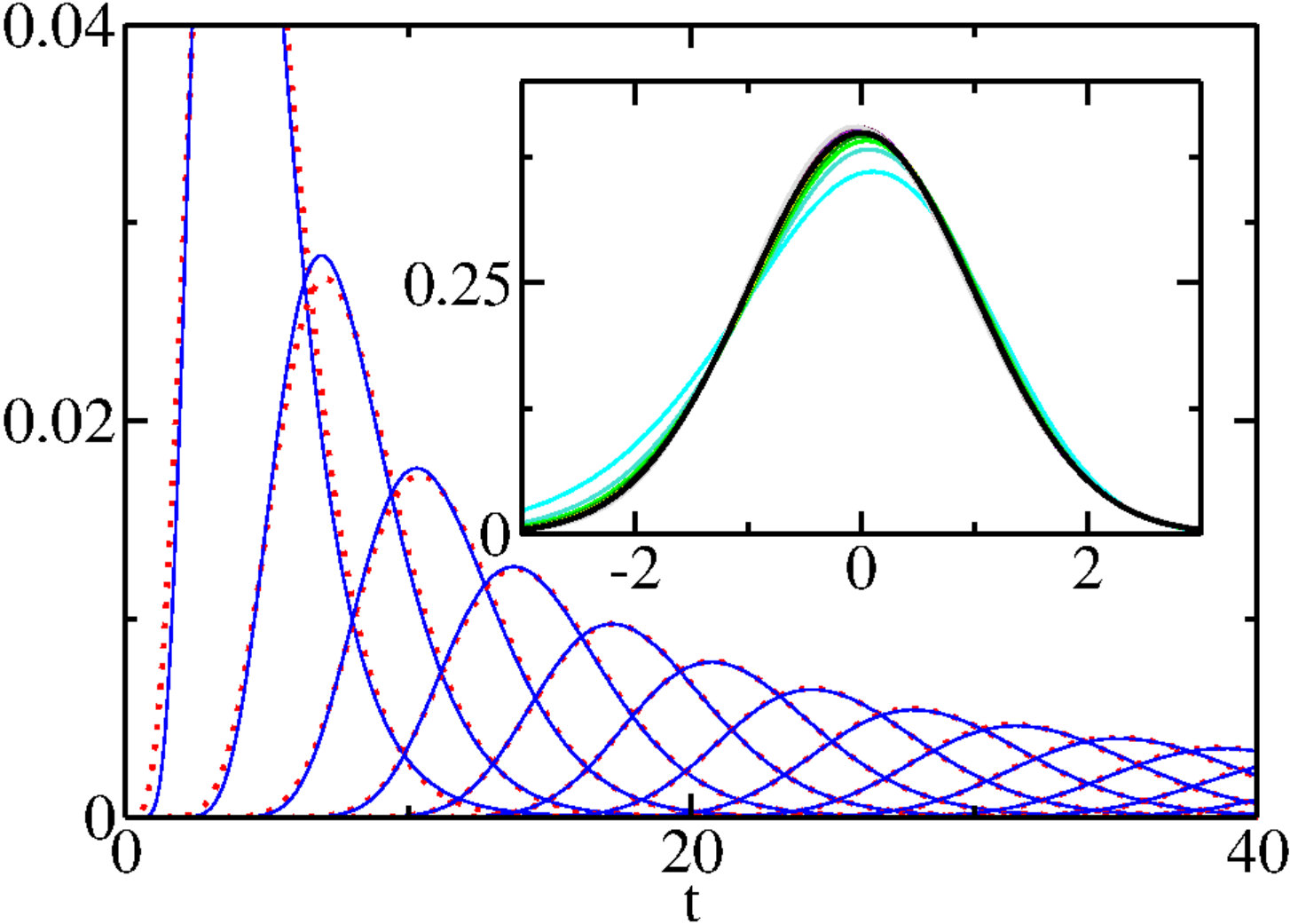 Figure 1
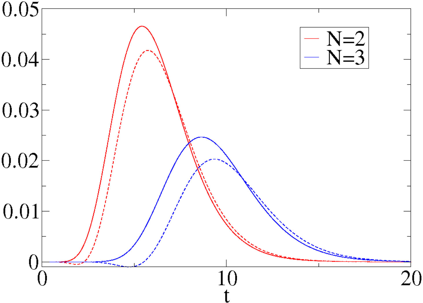 Figure 2
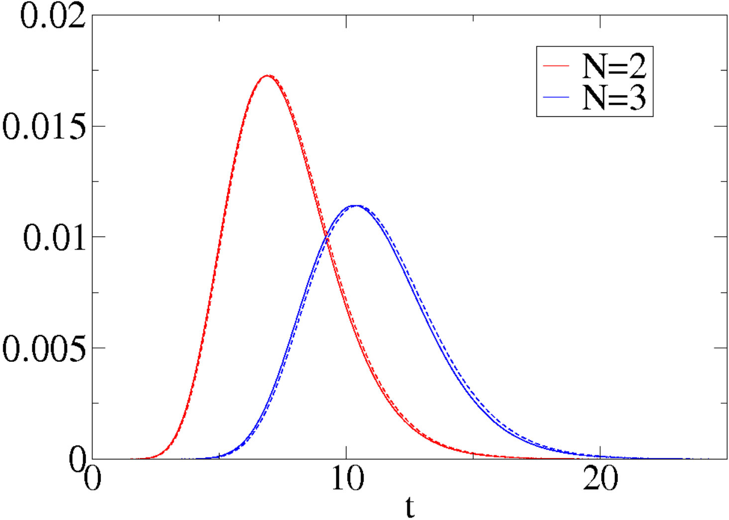 Figure 3
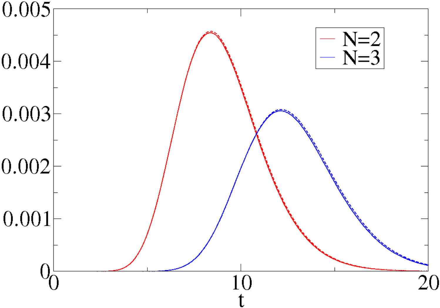 Figure 4
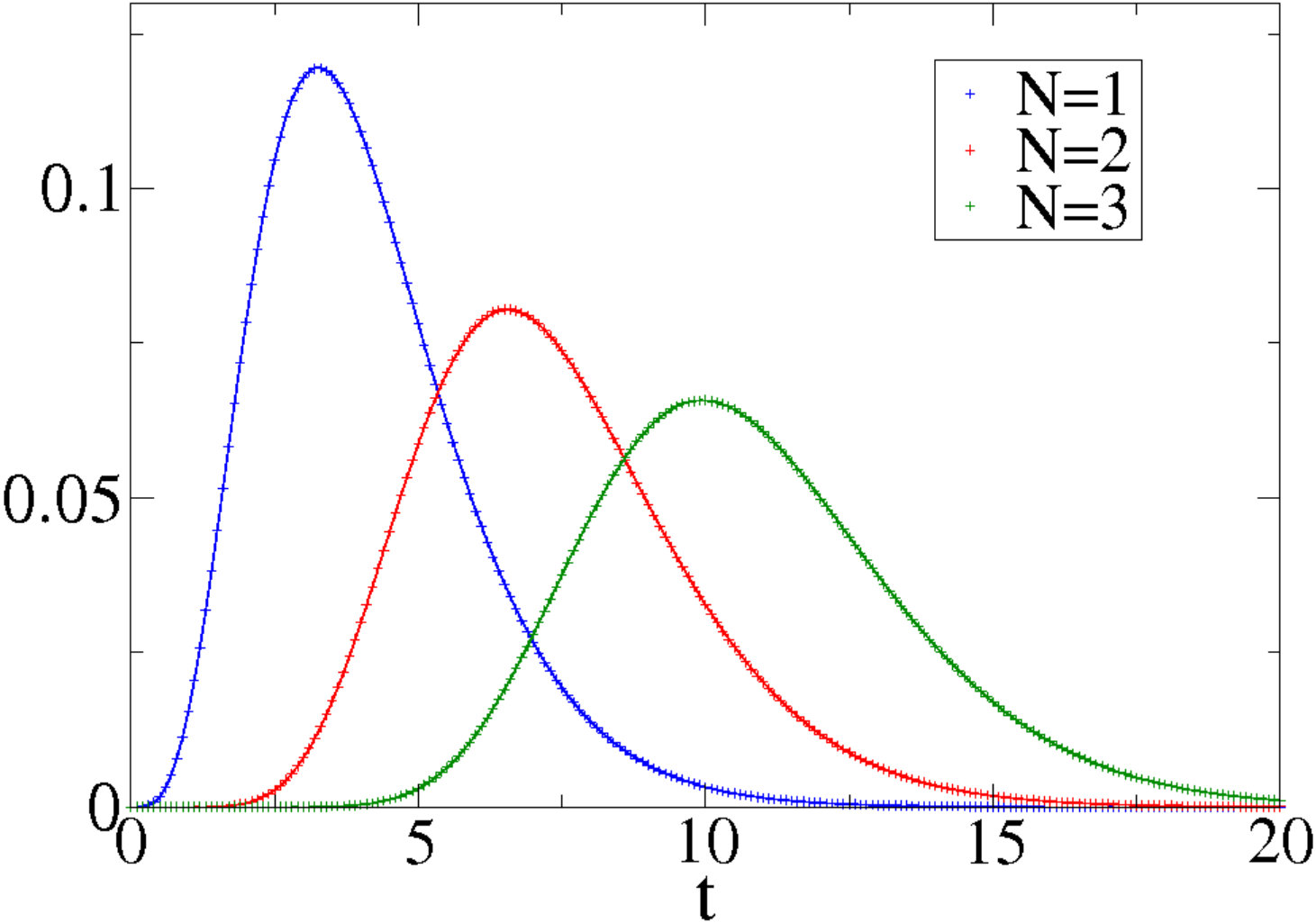 Figure 5
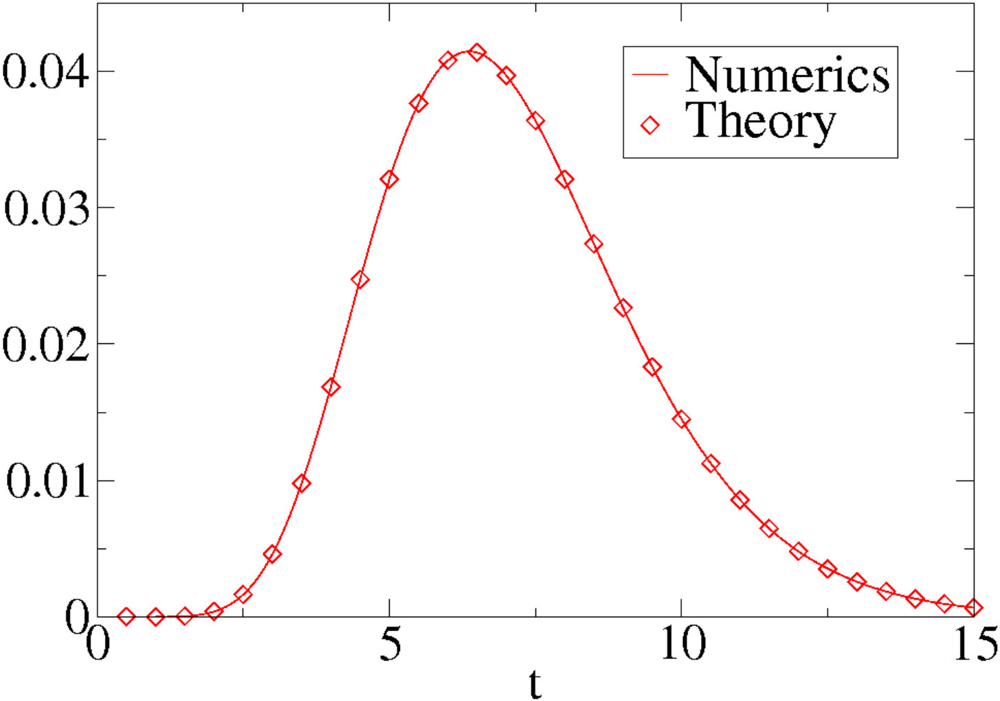 Figure 6
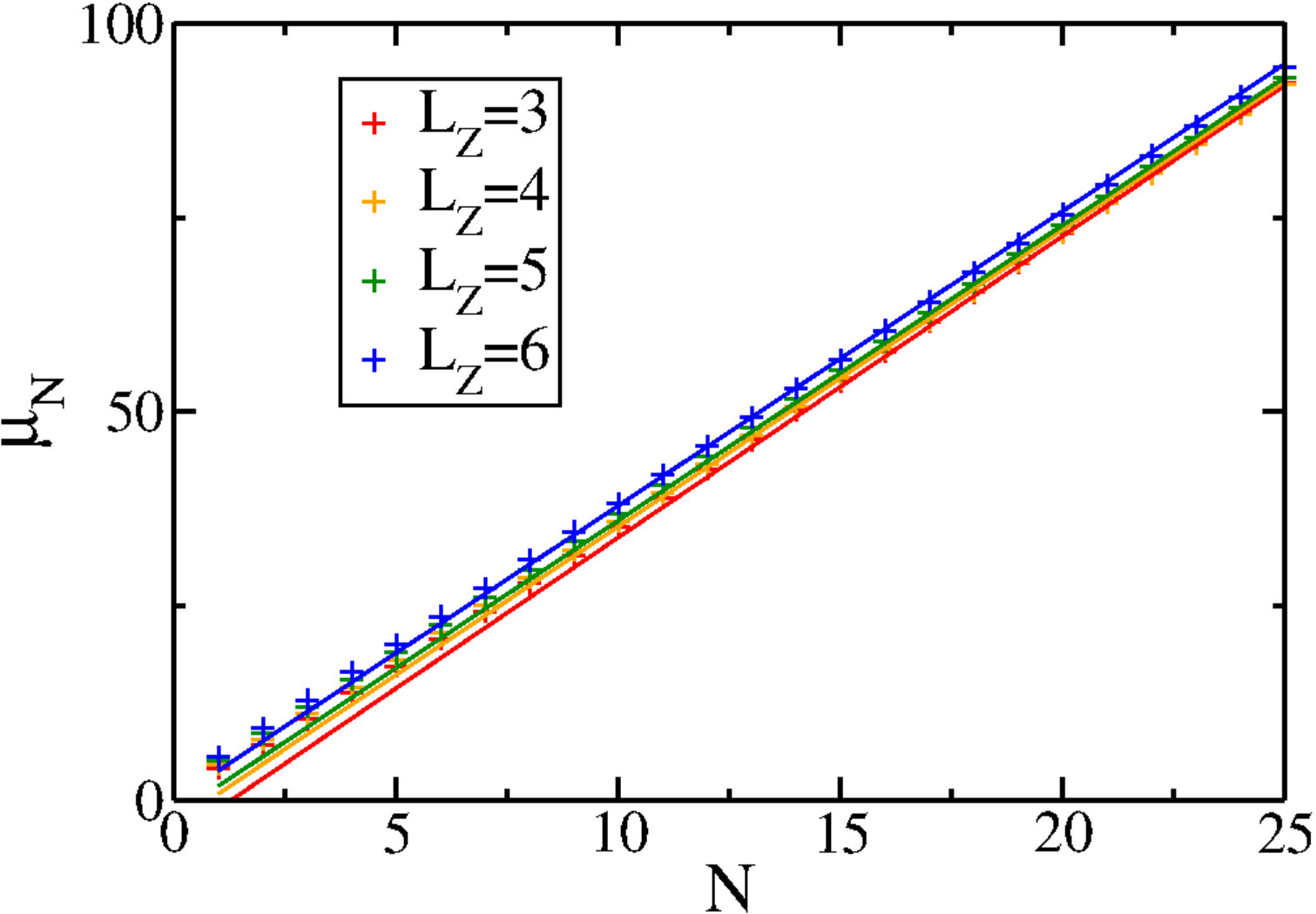 Figure 7
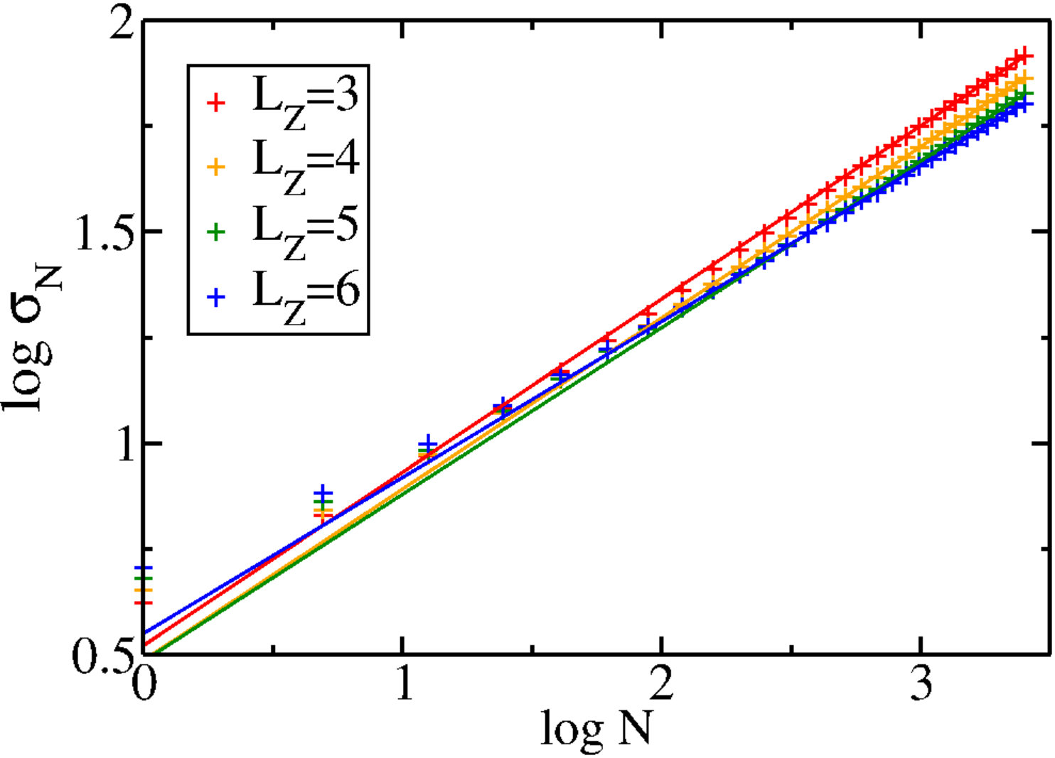 Figure 8
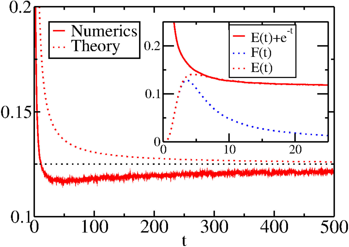 Figure 9
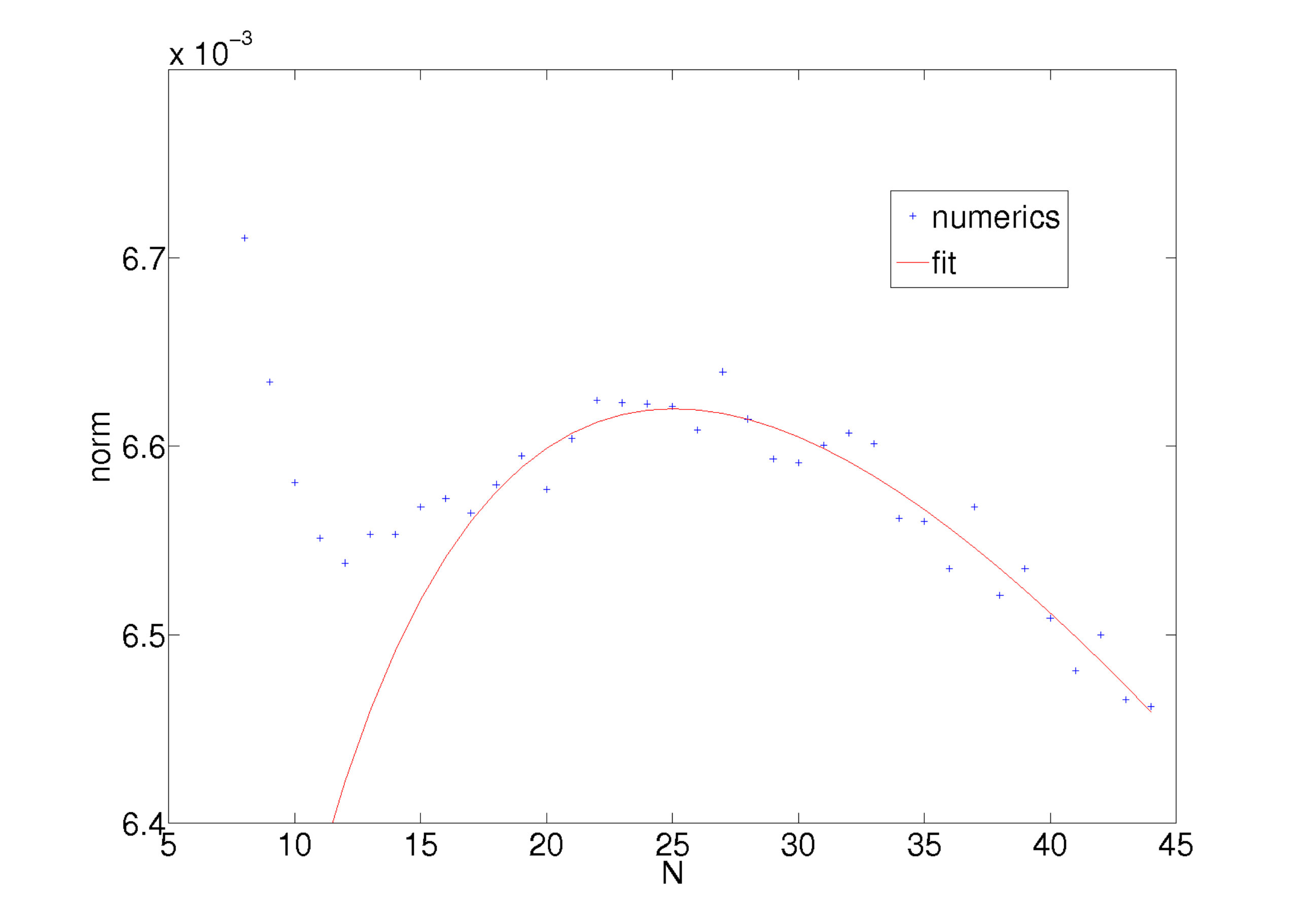 Figure 10
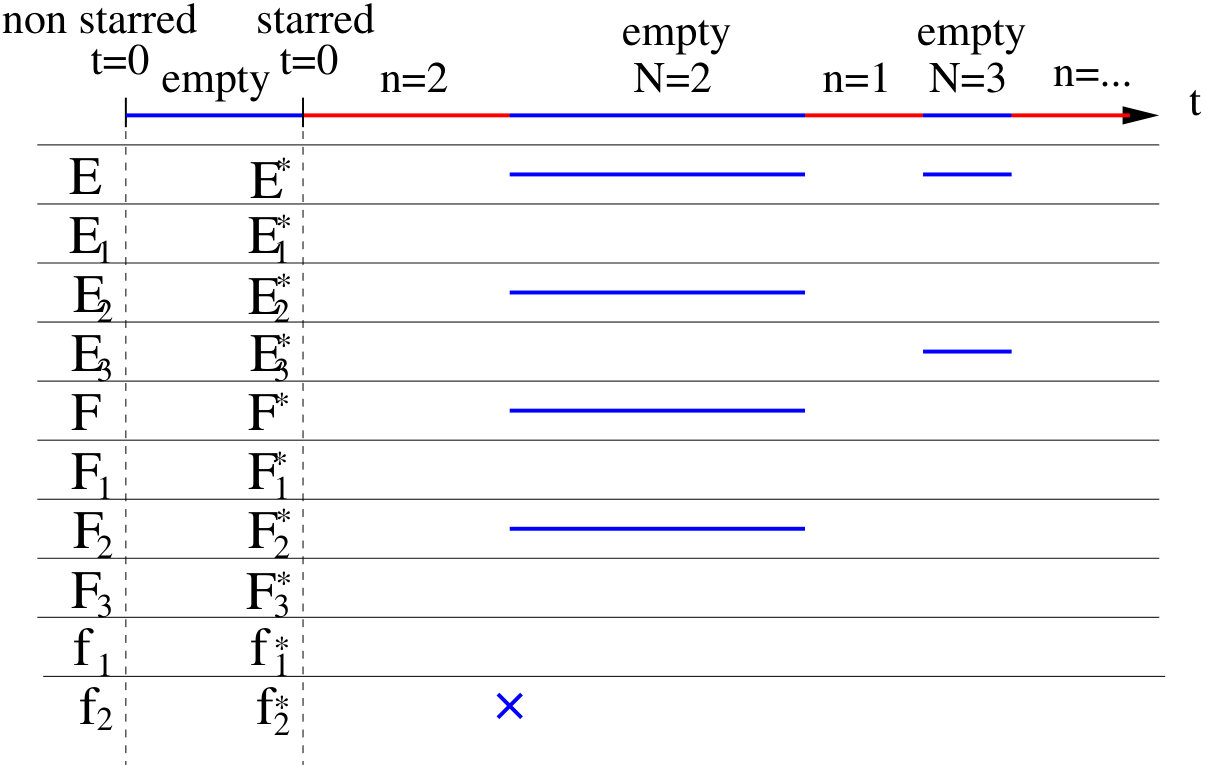 Figure 11
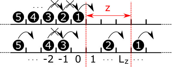 Figure 12
| 3 | 3.88 | -5 | 0.410 | 0.52 |
|---|---|---|---|---|
| 4 | 3.82 | -3 | 0.405 | 0.49 |
| 5 | 3.80 | -2 | 0.394 | 0.48 |
| 6 | 3.79 | 0 | 0.369 | 0.55 |
| ⋮ | ⋮ | ⋮ | ⋮ | ⋮ |
| 10 | 3.82 | 5 | 0.358 | 0.61 |
| ⋮ | ⋮ | ⋮ | ⋮ | ⋮ |
| 15 | 3.88 | 10 | 0.323 | 0.68 |
Peer Reviews
No public reviews on file for this paper yet. If you reviewed it on a platform where reviews are public (OpenReview, ICLR, NeurIPS, ICML), you can paste yours below so the community can read it here.
Videos
No videos yet. Explain this paper in a talk, walkthrough, or lecture? Add one.
Zone clearance in an infinite TASEP with a step initial condition
Julien Cividini1, Cécile Appert-Rolland1
1 Laboratoire de Physique Théorique, bâtiment 210 Université Paris-Sud and CNRS (UMR 8627), 91405 Orsay Cedex, France
Abstract
The TASEP is a paradigmatic model of out-of-equilibrium statistical physics, for which many quantities have been computed, either exactly or by approximate methods. In this work we study two new kinds of observables that have some relevance in biological or traffic models. They represent the probability for a given clearance zone of the lattice to be empty (for the first time) at a given time, starting from a step density profile. Exact expressions are obtained for single-time quantities, while more involved history-dependent observables are studied by Monte Carlo simulation, and partially predicted by a phenomenological approach.
Although it has been proposed first for biological applications [6], the Totally Asymmetric Simple Exclusion Process, or TASEP, has quickly become a paradigmatic model of out-of-equilibrium statistical physics and of stochastic processes [7, 8]. It has been shown to be a minimal model for various transport processes, for example in biological systems [9, 10] or in car traffic [11, 12]. The TASEP consists of point-like particles hopping on a one-dimensional discrete lattice. Particles hop only to the right, and only if the target site is empty. Though the model definition is very simple, the model has nevertheless a very rich behaviour, exhibiting boundary driven phase transitions. The TASEP has mainly been studied with periodic or open boundary conditions, or on an infinite line.
The role of defects has been extensively studied in the TASEP [13, 14, 15, 16, 17, 18, 19, 20, 21, 22]. In several applications the defects are dynamic and may depend on the local configuration of particles. A particular case of such defects is given by on- and off-gates. In the case of pedestrians, such a gate could for example result from a counterflow or a competing flow temporarily blocking the access to a bottleneck [23, 24, 25]. Some processes regulating protein synthesis along mRNA strands could also be modelled by such on- and off-gates [17]. In these two examples, the temporary closure of the gate can occur only if a certain region (which we shall refer to as the clearance zone) is void of particles. Once closed, the gate prevents particles to pass until it opens again. If enough particles accumulate behind the gate during the closure, an efficient transient flow takes place at the opening, with an initial condition that can be approximated by a step [23]. Predicting the probability that during this transient, the clearance zone could be empty - and thus allow for a new closure of the gate - is an open question. The work presented in this paper can be seen as a first stage to study this coupled dynamics between closure of the lattice and positions of the particles.
In this paper, we shall consider the TASEP on an infinite line (or infinite TASEP), with a step initial condition (namely all the sites to the left of a given site are occupied and all the others are empty at initial time). For the TASEP on an infinite line, the propagator of the system can be derived exactly by Bethe Ansatz and takes the form of a determinant [26]. Besides, in the case of the initial step condition, exact results can be obtained, in particular for the statistics of the particle current, and much effort has been made to obtain the asymptotic behavior of e.g. density profiles or the large deviation function of the current in the limit of large times [9, 27, 28].
The observables we shall be interested in are the probabilities that a certain zone of the lattice located to the right of the initial step is empty, or empty for the first time. These probabilities will be computed either regardless of the past history or with the requirement that the zone has always been occupied before.
In section 1 we define the infinite TASEP with a step initial condition and outline some useful results from the literature. Section 2 is then devoted to the motivation and exact definition of the model. In particular we shall define a clearance zone and the probabilities associated to the zone being empty. Exact and phenomenological analytic results are then presented in section 3 and numerical ones in section 4. Section 5 concludes the paper.
1 TASEP with a step initial condition
1.1 The model
The TASEP is defined on a one-dimensional lattice, whose sites may be occupied or not by a particle. During time evolution particles are allowed to hop from the site they occupy towards the site directly to the right, say from site to , provided this latter site is empty (not occupied). The system therefore satisfies the simple exclusion constraint, i.e. there is a maximal number of one particle on each site at any time. In this work we choose to evolve the system in continuous time, where all the allowed transitions occur with the same constant rate . Equivalently, waiting times between hopping attempts are drawn from an exponential distribution with parameter .
Here we will consider the TASEP on an infinite line. We shall study the relaxation of a step initial condition, see Fig. 1. At initial time, all the sites to the left of a given site are occupied and all the sites to the right are empty.
Sites are labeled by integers ranging from to . We write if site is empty and if site is occupied at time . Setting the discontinuity between sites [math] and , the initial condition reads
[TABLE]
Equivalently, the state of the system may be described by the positions of the particles that occupy it. More precisely, we label the particles with a positive integer from right to left. The state of the system at any time is therefore described by a formally infinite vector and the initial condition reads
[TABLE]
Notice that the positions of the particles are ordered at all times, i.e. for all . Here the only rate in the system is , and time may be rescaled to set , which we shall do in the following.
Numerically, the system is simulated by evolving the vector of the positions of the first particles in continuous time using Gillespie’s algorithm [29]. As the motion of one particle is not influenced by the particles on its left, the numerical measurement of any observable involving only the first particles will be free of finite size effects. For other observables for which the number of particles which are involved is not known a priori, one must check that enough particles are simulated. It is possible to verify during the simulations that the leftmost simulated particle does not move during any of the realizations of the Monte Carlo simulation, to ensure that the measurements are free of finite-size effects. In practice, simulating a step initially from to gives negligible finite-size effects for all results presented in this paper.
In the next subsection we review some theoretical results on the TASEP that we will use in the following.
1.2 Propagator
The propagator of the infinite TASEP with a finite arbitrary number of particles has been obtained in Ref. [26] by solving the master equation. The dynamics is obviously invariant under time translations, so that the propagator depends only on the difference between the initial and the final time. The probability to reach configuration starting from then reads
[TABLE]
where we keep track of the number of particles and the functions will be defined shortly. We also stress the fact that the propagator (3) exactly describes the motion of particles to since the motion of particles with has no effect on the first particles. It is manifest in (3) that the system is invariant under spatial translations.
The have the following expression [26, 30]
[TABLE]
where and is a contour that encloses both potential singularities [math] and . It is clear from (4) that for and . The have several remarkable properties listed in Ref. [26]. In the following, we will in particular use
[TABLE]
Simple arguments show that at long times if and for and . Finally, the first few , which we will need later, read
[TABLE]
where if assertion is true and [math] otherwise, and it is understood that a sum with ill-ordered bounds vanishes. In particular, the number of hops of an isolated particle follows a Poisson law for .
As the dynamics of a TASEP particle is not influenced by its successor, the results presented here for finite may as well be applied to a system with an infinite number of particles. More precisely, starting from a semi-infinite step at time , the probability to find the rightmost particles at positions at time is , where is defined by (2).
From there, the expression of the probability that the particle has hopped at least times by time was found to be [31]
[TABLE]
The first equality comes from the definition of the propagator, the second one is the technical step, in which the sums are decoupled using (5) and the antisymmetry of the determinant. At the third one the summations are performed columnwise using (5) again, and the fourth one is simply a shorthand that stresses the fact that all the indices of the have simply been increased by compared to the propagator (3). More details on the calculation can be found in Refs. [31, 30].
The previous results give information about the correlations between sites at a given time. There are also results about some other types of correlations, for example for the positions of a given particle at different times [32]. However, the general correlation for any times/positions is not known.
1.3 Hydrodynamic profile and maximal current
The properties of the system at long times have been investigated using the hydrodynamic approximation. At scales very large compared to the lattice spacing, the variable can be replaced by a continuous space variable . In order to describe the system at the large scales, one defines the density field . In the case of the TASEP, at large times the evolution of the density profile is described to lowest order by Burgers’ equation [33, 34].
[TABLE]
with the initial condition . The solution of the Burgers’ equation then reads
[TABLE]
Actually there are fluctuations around this profile, which have been characterized in [35, 34]. In the long time limit, around the position of the initial step, the density profile will flatten and tend towards , while the corresponding current will tend towards .
In the next sections our interest is to find the probability for a given zone (that we shall call * clearance zone* in the following) to be empty, possibly for the first time. This requires, firstly, to characterize better the short time behavior and, secondly, to account for some time correlations. Though the results of subsection 1.2 are valid at all times, the focus of most of the applications of these results was on the long time behavior [30]. Besides, we are missing some information on time correlations.
2 Clearance zone
2.1 Definition of the clearance zone
Problems in which a certain set of sites may or may not be accessible to the incoming particles arise in some applied TASEP-based models. In Ref. [17] Turci et al. studied a model for mRNA in which a zone could open or close at certain rates. In their model the lattice represents a mRNA strand and the particles represent ribosoms, which synthetize proteins by moving along the mRNA strand. The motion of the ribosoms may be blocked by some buckling of the mRNA or by other proteins that may attach on a specific region of the mRNA strand if this region is empty. This feature is accounted for in the model by defining a zone that corresponds to this specific region in the TASEP lattice, and can flip between open and closed states. As in the biological system, the blocking may occur only if the region is empty.
Jelic et al. studied a model of pedestrians in which two counter-propagating flows of pedestrians share a common bottleneck of several sites in which only one species can enter at a time [23]. The other species is then prevented to enter the bottleneck until the bottleneck-zone is empty.
In both examples, if the parameters are such that the clearance zone stays closed for a long enough time, impeded particles tend to accumulate behind the zone. The flow when the zone opens again is then very similar to the relaxation of a step profile.
We therefore believe that it is of interest to study a minimal version of this problem. For an infinite TASEP with a step initial condition as detailed in subsection 1.1, we define the clearance zone as the set of sites ,,…,. The size of the clearance zone is the only parameter in the problem. Such a clearance zone is represented on Fig. 1. It can be thought as being closed until the initial time .
2.2 Probabilities to be empty
The first quantity of interest to us will be the probability that the clearance zone is empty, i.e. that at some given time . We will also be interested in the number of particles to the right of when the clearance zone is empty. All the subsequent definitions are illustrated in Fig. 2.
More precisely, we define as the probability that is empty at and that particles have passed through the clearance zone. In a more mathematical way
[TABLE]
We also define , the total probability that the clearance zone is empty at time .
Note that the sum defining starts with , i.e. one considers only the case of an empty zone after the passage of at least one particle through the clearance zone. There is actually a time interval starting at where is empty and no particle has gone through it. In the future we may want to change the time origin in order to eliminate this ’zeroth’ empty interval. We shall therefore consider an alternative definition of the initial time and define the and analogously to and , except that the initial time of the starred quantities will be taken at the end of the zeroth empty interval. The zeroth empty interval ends when particle enters the clearance zone by performing its first hop from site [math] to site . The waiting time before the first hop is exponentially distributed, and the starred and non-starred quantities are related by
[TABLE]
for and similar functions to be defined later (which will all verify , a condition for (11) to hold) . Eq. (11) may be inverted to give
[TABLE]
Equivalently, the initial condition for the starred quantities is
[TABLE]
In some models the clearance zone is allowed to close when it is empty, so that histories where there exist empty intervals will have modified weights compared to what the model studied here would give. As a first step to account for it, we shall also be interested in the first time is empty (not considering the zeroth one), though no closure will be considered in the present paper. We define as the probability that is empty at time , conditioned by the fact that belongs to the first time interval where is empty, and that particles have passed. We also define , the and in analogy with the quantities. We have , with the special case .
Finally we also define the , and their starred counterparts as the probabilities that becomes empty for the first time between and with particles passed. The clearance zone almost surely gets empty for the first time at some moment of time, which imposes
[TABLE]
Eq. (14) is true when replacing by as well.
A quantity similar to has been introduced in Ref. [36] and extended in Ref. [37, 38], in a model in continuous space, where particles are injected at the entrance of a one-dimensional channel and cross it with a constant velocity until they reach the exit. In their model clogging occurs if more than one particle is present at the same time in the channel, and the authors derive various exact formulas for reversible [36] or irreversible [37] clogging, including the probability that no clogging occurs until a given time in the irreversible case. Adapting this simple Markovian model to our case would give an exponential distribution for .
The characterization of the and quantities will be the main goal of this paper. Obviously the knowledge of a non-starred quantity is equivalent to the knowledge of its starred counterpart, so that we shall use the most convenient set of functions, depending on the situation. It is also readily noticed that the quantities are single-time correlation functions and are expected to be a lot easier to compute than the quantities, which depend on the whole history of the system.
In the following we present a combination of exact, approximate and numerical arguments that account for the main properties of the probabilities defined in this subsection.
3 Analytic results
3.1 Direct calculation for
Here we focus on the simplest case , where all the quantities of interest can be computed directly, for an arbitrary length of the clearance zone . In this section we shall show how to compute , while the expressions for and , that can be obtained analogously, will be given in A. By definition of we track the events where and and calculate their associated probability. By definition of the starred quantities, particle is on site at . Since and the motion of the second particle is not influenced by particles , we may restrict ourselves to a -particle system with and . We define two remarkable times: the time when particle hops from to will be denoted and the time when particle hops from to [math] (if it does) will be denoted . For the history to contribute to , we must obviously have .
We shall now compute the probabilities of the histories that will contribute to . We first consider the case . The probability to have a given value of and any value then reads . In that case particle is necessarily blocked on site [math] until hops at time . After that, the events that contribute to are those where particle does not hop during an interval of length , with associated probability , while particle must have hopped for the time at time exactly , which occurs with probability .
In the second case , the probability to have a given value of and a value of such that is . Particle is then allowed to perform at most one hop between and , corresponding to a probability to perform respectively [math] or hop.
The sum of these two terms reads
[TABLE]
where is the upper incomplete gamma function and is Euler’s gamma function.
From Eq. (3.1) we see that decays as at large times. In a naive reasoning we could consider that the events contributing to the long time behaviour of are those where particle goes very slowly through the zone and particle does not enter the clearance zone. However the impediment of two particles would give a contribution . Actually, the dominant contribution is given by events where particle blocks particle most of the time. This requires the blocking of only one particle, hence a probability .
This combinatorial method provides an intuitive way of computing . It however seems hard to extend to . This shall be done in the next subsection by using the exact expression of the propagator.
3.2 The determinantal formula
Here we will see that an exact formula can be found for the on the basis of the exact expression for the propagator (3) and on the result (1.2).
For determining for a given one only needs to consider the first particles. We have
[TABLE]
By a trick similar to the one used in equation (1.2), the summations over the with may be decoupled and carried out, resulting in an increase of the index of the in columns of the matrix. We get as an intermediate result
[TABLE]
with
[TABLE]
The sum over only affects the first column and can be carried out, using (5) once again. We finally get
[TABLE]
with
[TABLE]
The result (19)-(20) is exact, and can be checked to give Eq. (A) for . The first few are plotted in Fig. 3. The agreement with the numerics is excellent as expected.
Eqs. (19) and (20) give a compact exact solution to part of our problem. These expressions however involve determinants and are not very easy to manipulate. In particular, it is not clear how to find a compact expression for starting from (19)-(20).
3.3
It was already mentioned that the are more complicated quantities than the because they depend on the whole history of the system. In principle exact expressions could be written by summing over intermediate variables. Here we simply do it for to illustrate the idea. We also derive the asymptotics of at large times.
To compute we have to select events such that when the first particle exits the second already entered it. We denote as the moment when particle exits the clearance zone, and as the state just before the hop (state at time ). We have to enforce the following constraints on :
- •
Particle is supposed to hop from to at time , therefore .
- •
The clearance zone cannot be empty after particle hops. We therefore need .
- •
The clearance zone must be empty after particle leaves it, therefore particle cannot enter it. Consequently we must have at all times and in particular .
At time particle hops, with probability . Between time and time the second particle is supposed to exit . Following the same logic, at time the positions of the particles satisfy the following constraints:
- •
Particle has not yet entered the clearance zone, .
- •
Particle has exited, , and particle is ahead of it .
All these constraints can be expressed by the formula
[TABLE]
where we have integrated over all the possible times when particle exits. Fig. 4 shows the agreement between the exact expression (21) and numerical results.
Although this expression is complicated, its asymptotic behavior for large times may be extracted. In B we show that at large times we have
[TABLE]
Eq. (3.3) provides us with an equivalent of for long times. It can be shown that terms coming from sectors where one of and is finite are subdominant. This exponential part of the decay generalizes to higher values, as we expect to be a convolution of polynomial factors times simple exponentials, which combine to finally give an overall . The power law in front of the exponential seems harder to predict for general .
In the following subsection we try to find a more systematic, yet approximate method for computing the .
3.4 Approximate recurrence formula
In this section, in order to calculate the , we shall make an approximation that we expect to be all the more relevant as the zone gets larger. We first assume that the history of the system can be factorized as a product of histories over the intervals where is empty and where is occupied, and we assume that a step is reformed each time the clearance zone is empty. The durations of empty intervals are therefore drawn from a distribution
[TABLE]
where is the time needed to occupy the clearance zone again.
Based on the above assumptions, we may now write two series of identities that link the unknown functions , and . The first one reads
[TABLE]
Equation (24) means that the system is in the first empty interval at time if it has been emptied at time for the first time and no particle entered until then, i.e. the time at which the next particle will enter the clearance zone is larger than .
The second identity is typical of first-passage problems. It links the , the and the ,
[TABLE]
Eq. (25) states that if is empty at time , either it is the first empty interval or the first empty interval started at some time and the zone has been occupied again since then.
The can be eliminated by using the starred quantities and using (23). After these transformations, (24)-(25) imply
[TABLE]
We already know an explicit expression (19)-(20) for the . Equation (26) can therefore be used to compute the . For the convolution in time we define the shorthand . In this notation Eq. (26) reads . Using one can express the as a function of the ,
[TABLE]
Eq. (26) may be inverted for arbitrary . If we parametrize the partitions of the integer by a set of numbers such that the integer appears times in the partition, the satisfy . With this notation the general formula reads
[TABLE]
where is a multinomial coefficient.
The relations (3.4) and (28) may be tested numerically. The results are shown in Fig. 5, and it appears that the approximations (24) and (25) work better and better with increasing . Indeed, histories where becomes empty after the particle passes are most probably histories where the particle has been blocked for a long time, hence an accumulation of particles behind. The larger the clearance zone, the longer the time particle has been blocked, the higher the density is likely to be on sites . For larger clearance zones the density profile is therefore closer to a step and the recurrence approximation indeed works better.
4 Numerical results
4.1 Quantities summed over
A seemingly simpler problem concerns the summed quantities , and , . We first note that, within the frame of the recurrence (24)-(25), a simple relation exists between and . Equation (26) can be summed over to give
[TABLE]
We therefore focus on .
Although we have derived exact expressions for the , it is not clear how to sum over to obtain a useful expression for . For predicting we try instead to make use of the hydrodynamic solution (9). The initial step lies between sites [math] and , so that we expect
[TABLE]
where the on the LHS is the probability associated to the zeroth empty interval, which we added for convenience, though it is vanishing at hydrodynamic times. Eq. (30) is compared to numerical measurements in Fig. 6.
On Fig. 6 there is a discrepancy between the hydrodynamic approximation and the numerics, which reveals that correlations exist. The two curves have the same limit , corresponding to the convergence towards a maximal-current phase where every site is occupied with probability . The hydrodynamic prediction however converges from the top while the numerical curve comes from the bottom. This effect can be attributed to the presence of long-lived spatial correlations. Denoting ensemble averages with the brackets , it is numerically observed that at large times two-point functions of the kind or are slightly larger than their stationary value , while those of the kind and are slightly smaller than . These correlations decay algebraically in time. As a consequence, since neighbouring sites are anticorrelated we have at large times.
For future applications to closing regions as mentioned in section 2, an important quantity is the summed probability that the clearance zone is in the first empty interval irrespective of the number of particles that passed. This quantity is shown in the inset of Fig 6.
From the study of the some properties of a system with infinite closing rate could be deduced. For instance, the probability that the clearance zone has closed at time would be equal to .
4.2 Scaling properties for large
In this subsection we study numerically the scaling behavior of the for large . The are plotted for and in Fig. 9.
We start by measuring the norm and the first cumulants of the for a given value of . We define
[TABLE]
We now study the dependency of the three observables in , still for a given value of . For large , we see on Fig. 7 that the mean increases linearly and the variance increases algebraically . The case of the norm is more complicated and the discussion is delayed. In the fits for and , the coefficients are of course expected to depend on . Table 1 shows the best fitting parameters for several values. We shall now give some elements of interpretation of these coefficients.
For large , the mean of can be estimated as follows. The first particle typically needs time units to reach the end of , and after that we consider crudely that the current between sites and is constant equal to between times and , where we neglect the duration of the empty interval after the particle exits. We therefore have , or , giving and . This explains the order of magnitude of , and of when becomes large. Indeed, if we suppose that is in maximal current phase then and , . The numerical measurements show that , and since can still be interpreted as the inverse of the average current we have , as can be expected for the transient regime. The constant is a subdominant term and is evaluated less precisely. We however notice that its variation with is compatible with the preceding discussion at large .
The values of and seem trickier to explain. Numerically we have , so that the standard deviation is lower than for a sum of i.i.d. variables. There is a negative feedback, that may come from the fact that when a particle does not hop for a long time, thus reducing the current, a denser region appears behind it which will create a current higher than expected afterwards.
The norms are defined as the time integrals of the . In the approximation (23)-(24), we have
[TABLE]
Thus the may be directly interpreted as the probabilities that the first empty interval occurs after the passage of particles. More generally, is the product between the probability that the first empty interval occurs after the passage of particles and the mean duration of this interval, as shown in C
The norms are rather complicated functions of . Naively one would expect that is a decreasing function of , as the zone is less and less likely not to have been empty before the particle passes. Actually it is a non-monotonous function, as seen on Fig. 8. We would like to guess a form for the large behavior. We have seen in subsection 4.1 that the probability that becomes empty at time is slightly less than , due to long-lived algebraic correlations. In other words, the clearance zone is slightly more likely to be empty for increasing large times, i.e. for increasing large . Hence we take as a guess
[TABLE]
where the are unknown constants. It can be shown that the expression (4.2) has a maximum. Indeed this is confirmed by the numerical results obtained for in Fig. 8. Numerical results show that the correction term increases with the size of the bottleneck, which makes the maximum more and more prominent as increases.
Numerically, we find that the shape of each is very close to a log-normal distribution,
[TABLE]
where we ensure that the mean and the variance of and are the same by setting
[TABLE]
To check how close to a log-normal distribution is, we rescaled the axes and plotted as a function of for every . The result is shown on Fig. 9 for . The curves for very low value of seem to get closer and closer to the Gaussian limit corresponding to (35), but as grows the sequence of curves slightly overtakes the Gaussian and seems to converge towards a different limit. The log normal distribution however remains a very good approximation.
5 Conclusion
In this work we have taken a simple well-known system, the infinite TASEP with a step initial condition, and we have studied the probability that a certain clearance zone becomes empty. The quantities we have focused on are non-stationary, finite-time and finite-space quantities. An exact analytic expression was obtained for the probability that the clearance zone is empty at a given time conditioned on the number of particles that passed the clearance zone. The sum of these contributions, i.e. the probability that the clearance zone is empty, was however harder to obtain in a simple form. This latter quantity was shown to converge only algebraically to its equilibrium value, as long-lived spatial correlations survive for a very long time.
A step was made towards computing even more complicated, history-dependent quantities such as the , defined as the probabilities that the clearance zone is in its first empty interval at time , with particles having exited it. While the case is special in that does not truly depend on the history, we presented an exact expression for in terms of the propagator. Using this expression we derived the asymptotic behavior of for large times and showed that the exponential part was proportional to , a feature that we argued to be true for any . We have proposed an approximate recurrence relation linking the to the already known , that works quite well for large enough values of . Finally, we measured the main characteristics of the and discussed their physical meaning.
This work can be seen as a first step in the study of more complex systems involving a clearance zone switching between open and closed states, in which closing can occur only if the clearance zone is empty [17, 23]. In this paper the clearance zone does not affect the dynamics of the particles. It would seem natural to enable the closing of with some rate, as in the model of Ref. [17]. The closing of the clearance zone in some realizations of the system history would however modify the probabilities in a way quite difficult to compute exactly as it would once again involve the past history of each realization. In the case of an infinite closing rate, our results already provide the distribution of closing times.
Acknowledgements
We thank T. Sasamoto and G. Schehr for useful discussions.
Appendix A Expression of
The expression of can be obtained by a reasoning similar to the one of subsection 3.1. The main difference is that particle must hop more than times between times and .
[TABLE]
By combining (11) and (A) we also obtain
[TABLE]
Appendix B Large time asymptotics of
We evaluate the two parts of (21) for large values of the time arguments and . It can indeed be shown by examination that no dominant term comes from the parts where or are of order . We first write
[TABLE]
Now remember (subsection 1.2) that all the with are either zero or bring a factor with them at long times, so that all the terms in the RHS decay like except for the second one. We have the asymptotic equivalents and for . For large the propagator appearing in (21) then behaves asymptotically as
[TABLE]
where for any time, as . We use an analogous method to estimate the second part of the RHS of (21). For this second half the summations over and can be performed right away using again the identity (5). In principle the summation over could be performed as well, but we choose not to do so for the moment. We get
[TABLE]
where and are two constants. The factors come from the fact that the become zero for and . The first condition is obviously always true, and the third one is always false for all the interesting cases . Combining the second condition with the summation intervals in Eq. (21), only the term with and survives. After performing the remaining sums the second term is shown to dominate. In particular is the dominant term because of the factor (40). This finally gives the result (3.3).
Appendix C Interpretation of
Here we give a precise argument that proves that may be interpreted as the product of the probability that the first empty interval occurs after the passage of particles with the average duration of this interval, denoted .
We introduce the moment when the clearance zone is empty for the first time and the state of the system at this moment. We also use the shorthand for the probability that is empty for the first time at time in the configuration , and we write for the conditional expectation. Then may be decomposed as follows,
[TABLE]
where the superscript on the sum over indicates that the sum is restricted to configurations in which exactly particles have exited the clearance zone, and .
Taking the integral over , we can exchange the integrals
[TABLE]
We now use the fact that is equal to the probability that is empty for the first time after passages, which is also . Defining , we get
[TABLE]
where is the probability that is empty for the first time in configuration . The factor is the probability that is empty for the first time in the configuration conditioned by the fact that exactly
Thus the whole sum over is equal to and we may finally write
[TABLE]
In the recurrence of subsection 3.4 we made the simplifying assumption , which gives for all . This yields
The reference list from the paper itself. Each links out to its DOI / PubMed record.
- 1[1]
- 2[2]
- 3[3]
- 4[4] T. Sasamoto, T. Imamura, Fluctuations of the one-dimensional polynuclear growth model in half-space, J. Stat. Phys. 115 (2004) 749.
- 5[5] B. Derrida, A. Gerschenfeld, Current fluctuations in one dimensional diffusive systems with a step initial density profile, J. Stat. Phys. 137 (2009) 978–1000.
- 6[6] C. Mac Donald, J. Gibbs, A. Pipkin, Kinetics of biopolymerization on nucleic acid templates, Biopolymers 6 (1968) 1–25.
- 7[7] B. Derrida, An exactly soluble non-equilibrium system: the asymmetric simple exclusion process, Phys. Reports 301 (1998) 65.
- 8[8] T. Kriecherbauer, J. Krug, A pedestrian’s view on interacting particle systems, KPZ universality and random matrices, J. Phys. A-Math. Theo. 43 (2010) 403001.