An alternative local polynomial estimator for the error-in-variables problem
Xianzheng Huang, Haiming Zhou

TL;DR
This paper introduces a new local polynomial estimator for error-in-variables regression problems that reduces bias and improves numerical stability, supported by theoretical analysis and empirical validation.
Contribution
It proposes an alternative estimator that avoids kernel transformation, with rigorous asymptotic analysis, an efficient implementation, and demonstrated advantages over existing methods.
Findings
The new estimator is less biased than existing methods.
It is numerically more stable in simulations.
The estimator performs well on real motorcycle crash data.
Abstract
We consider the problem of estimating a regression function when a covariate is measured with error. Using the local polynomial estimator of Delaigle, Fan, and Carroll (2009) as a benchmark, we propose an alternative way of solving the problem without transforming the kernel function. The asymptotic properties of the alternative estimator are rigorously studied. A detailed implementing algorithm and a computationally efficient bandwidth selection procedure are also provided. The proposed estimator is compared with the existing local polynomial estimator via extensive simulations and an application to the motorcycle crash data. The results show that the new estimator can be less biased than the existing estimator and is numerically more stable.
Click any figure to enlarge with its caption.
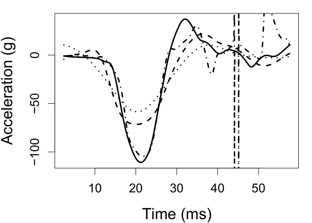 Figure 1
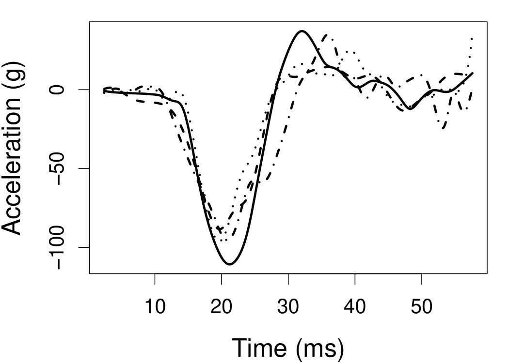 Figure 2
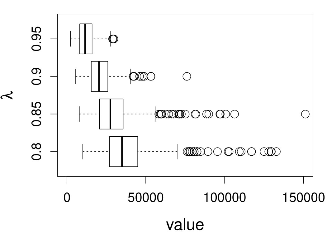 Figure 3
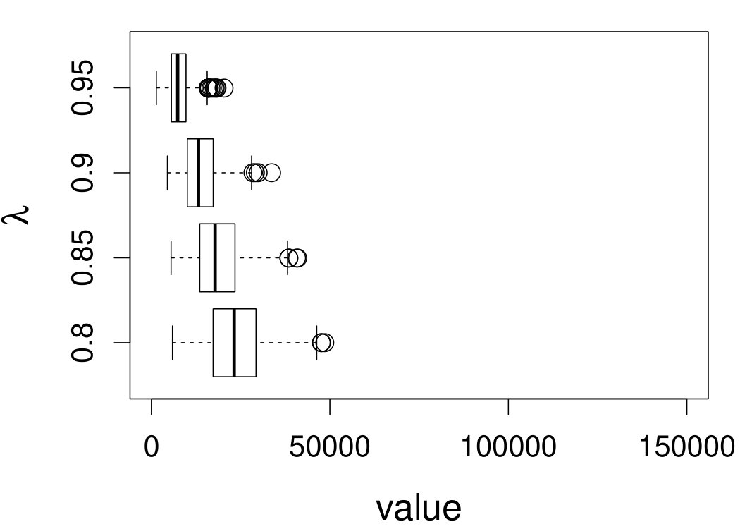 Figure 4
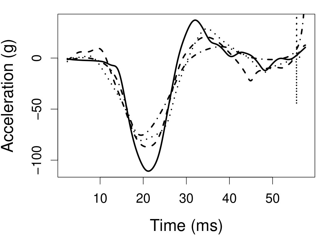 Figure 5
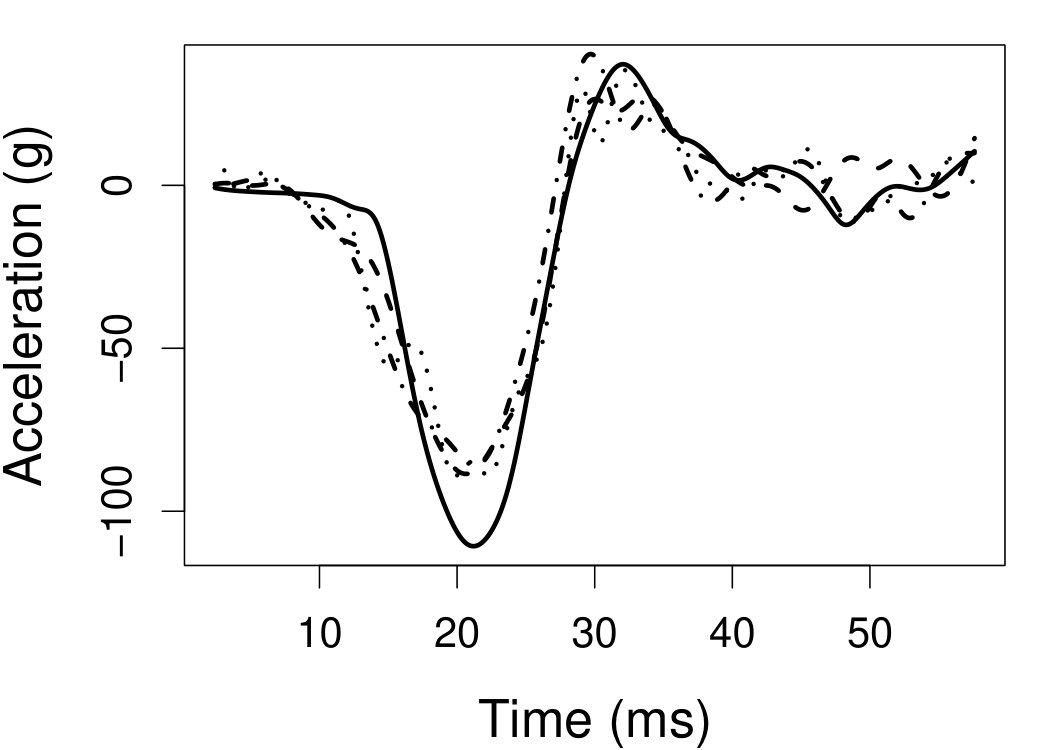 Figure 6
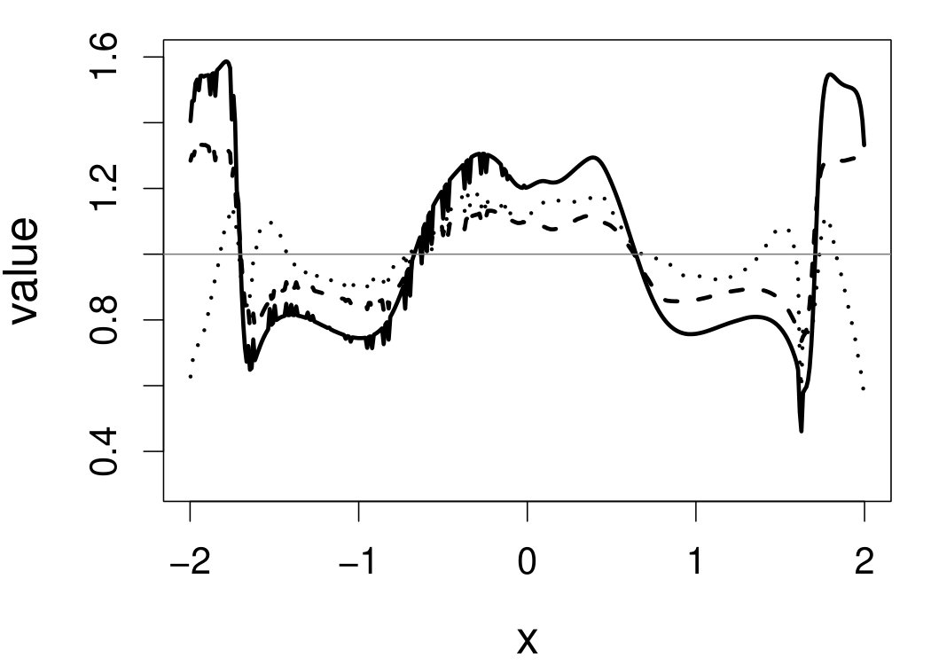 Figure 7
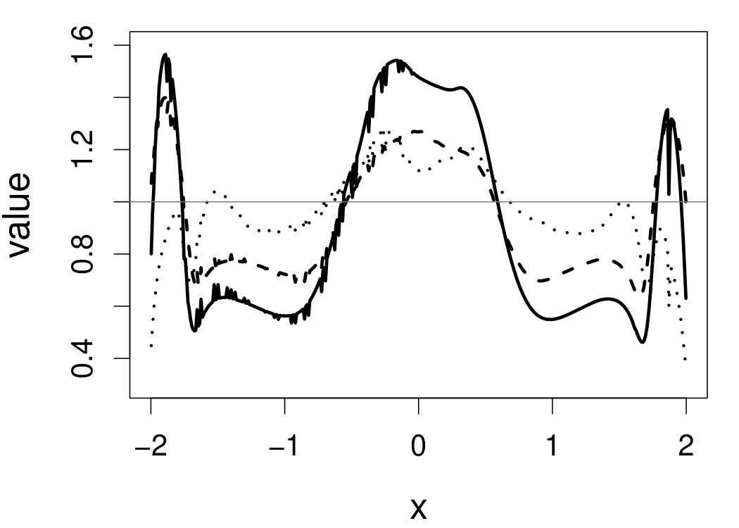 Figure 8
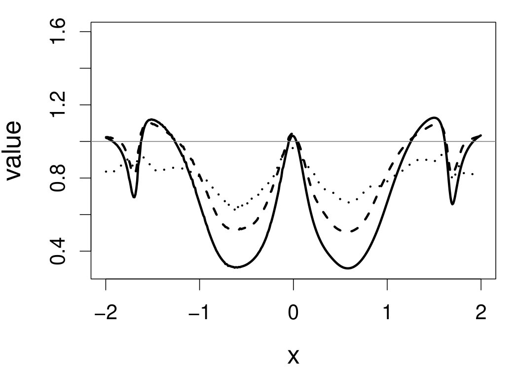 Figure 9
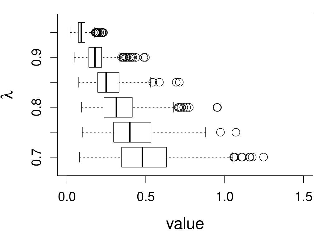 Figure 10
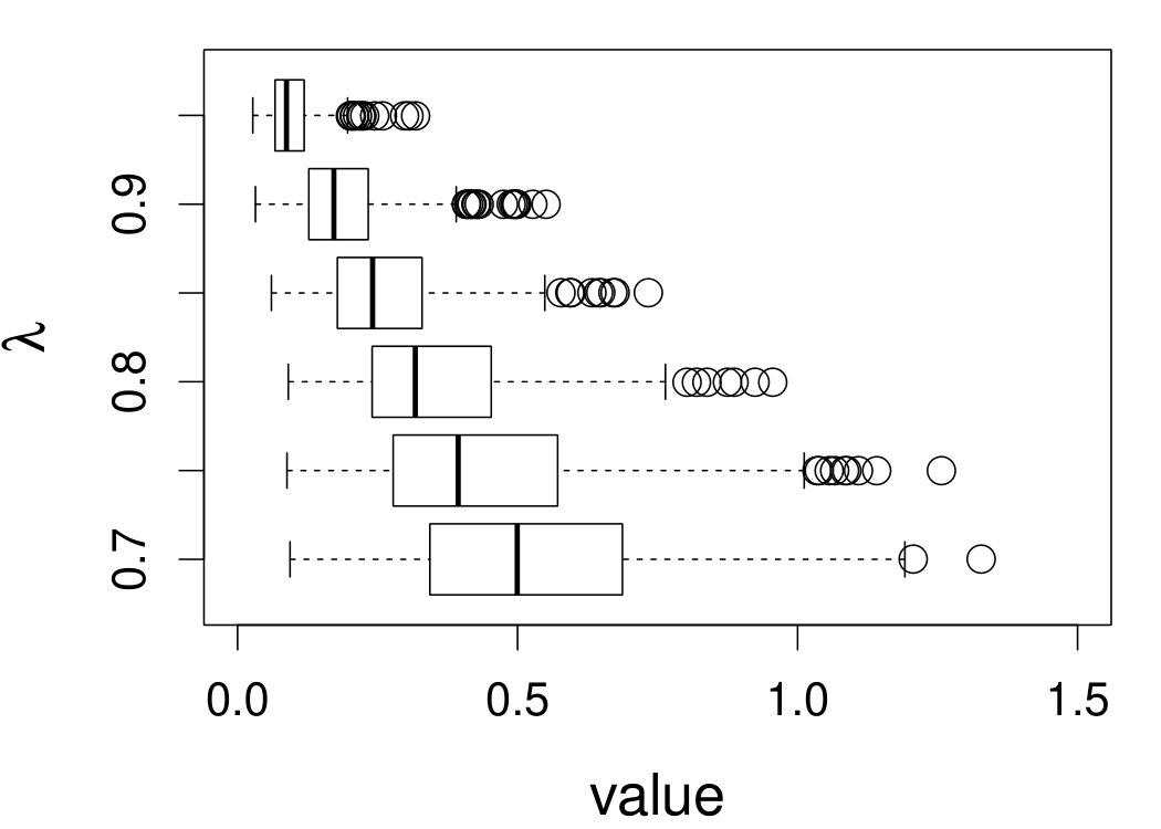 Figure 11
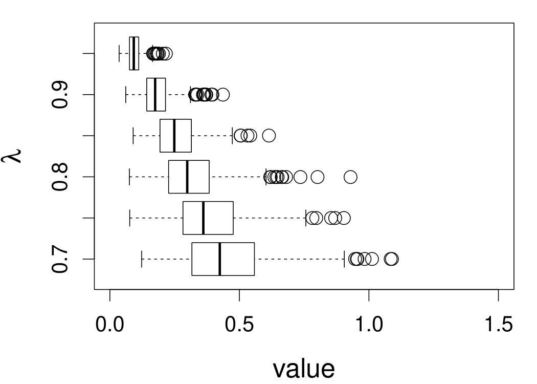 Figure 12
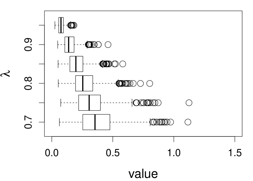 Figure 13
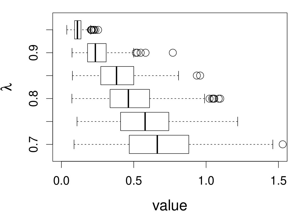 Figure 14
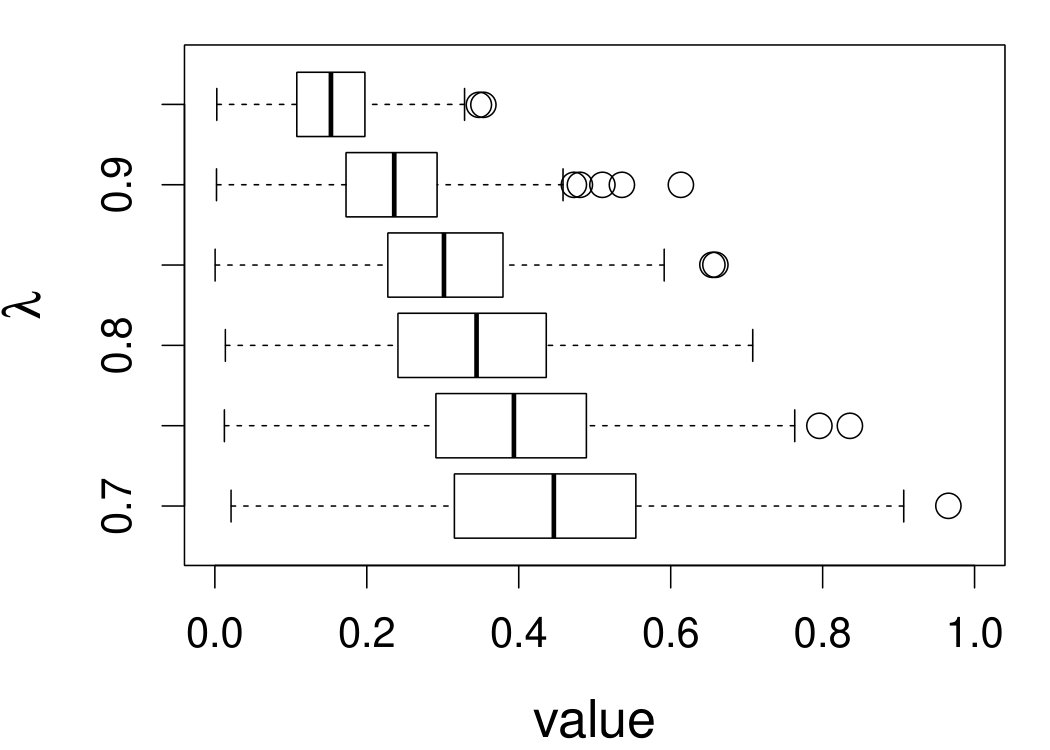 Figure 15
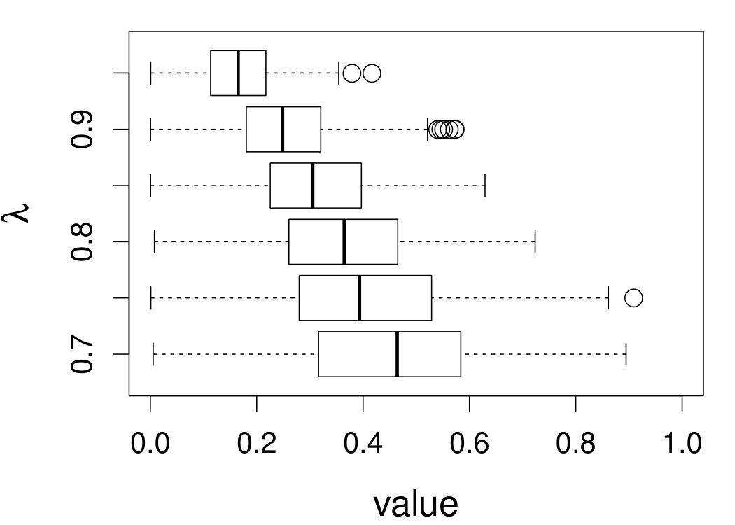 Figure 16
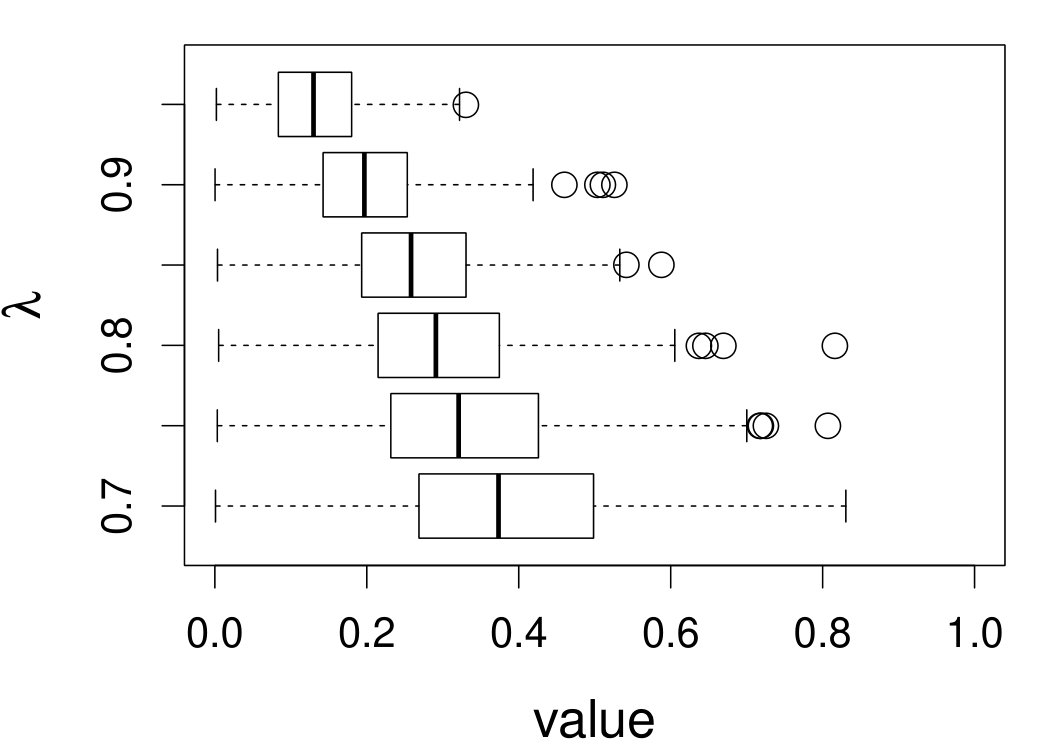 Figure 17
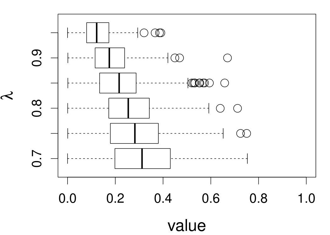 Figure 18
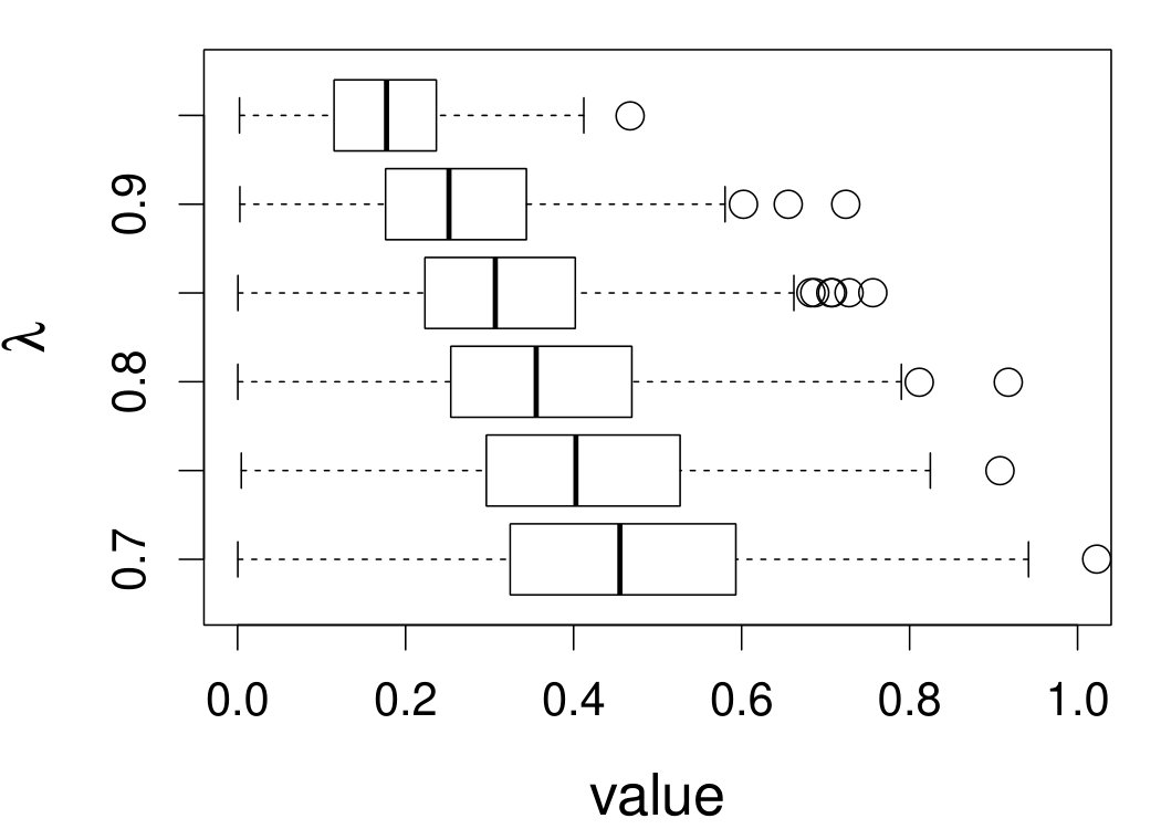 Figure 19
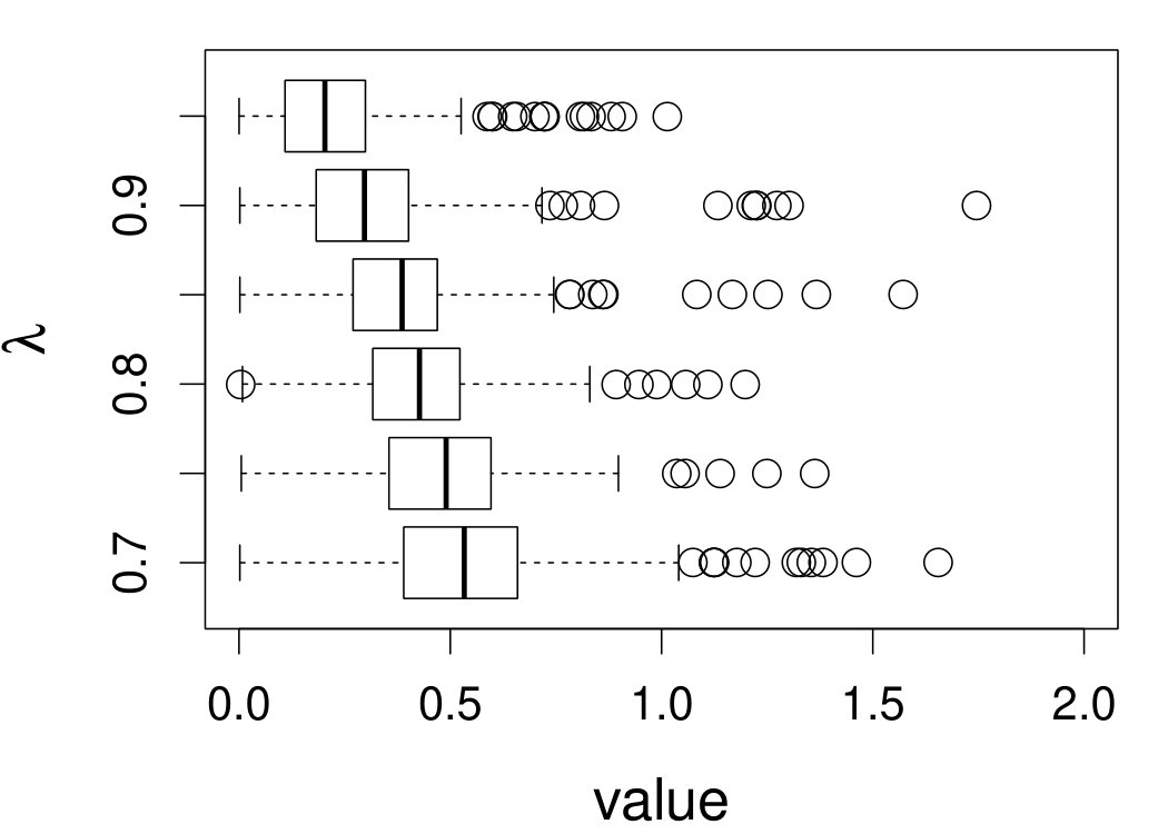 Figure 20
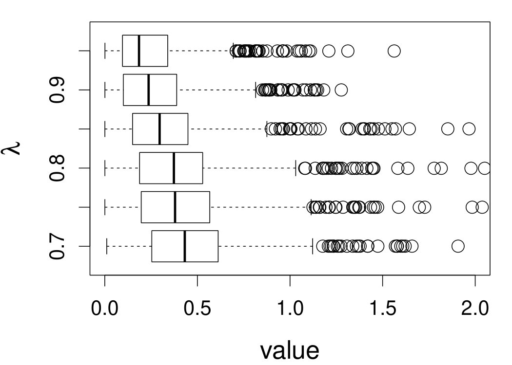 Figure 21
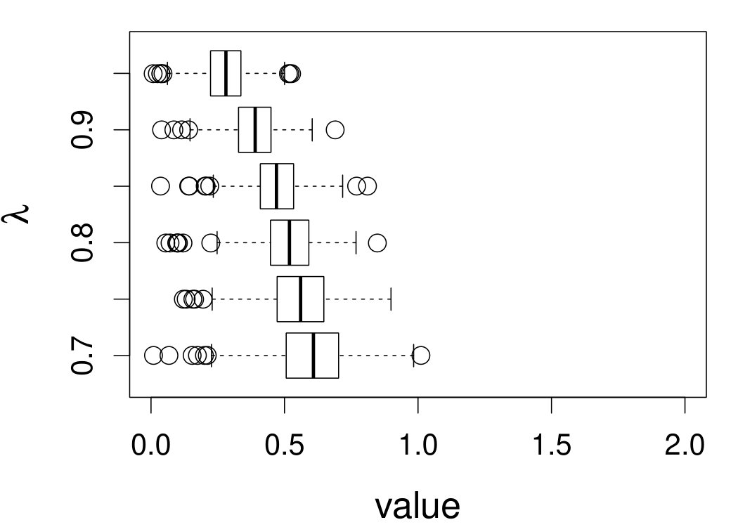 Figure 22
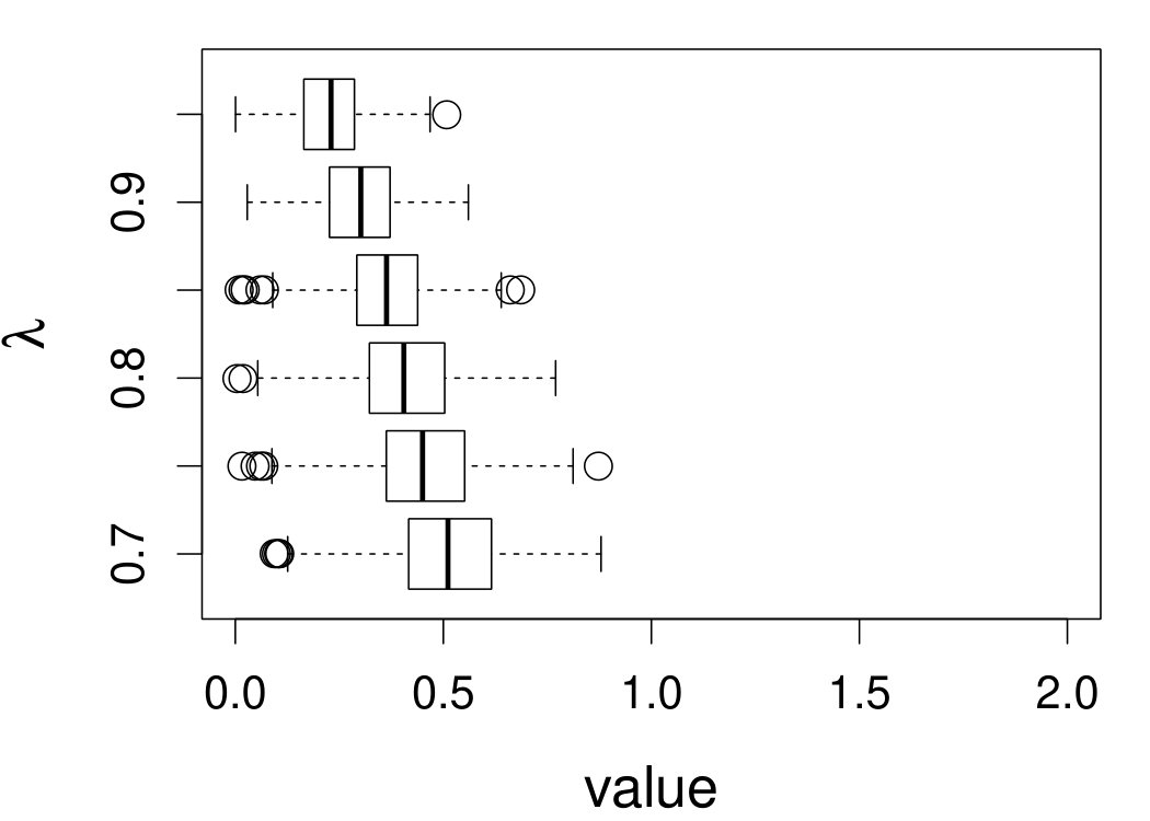 Figure 23
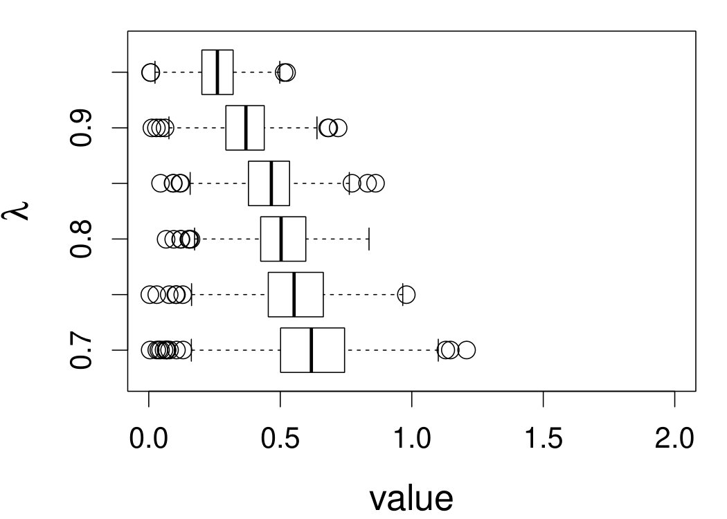 Figure 24
 Figure 25
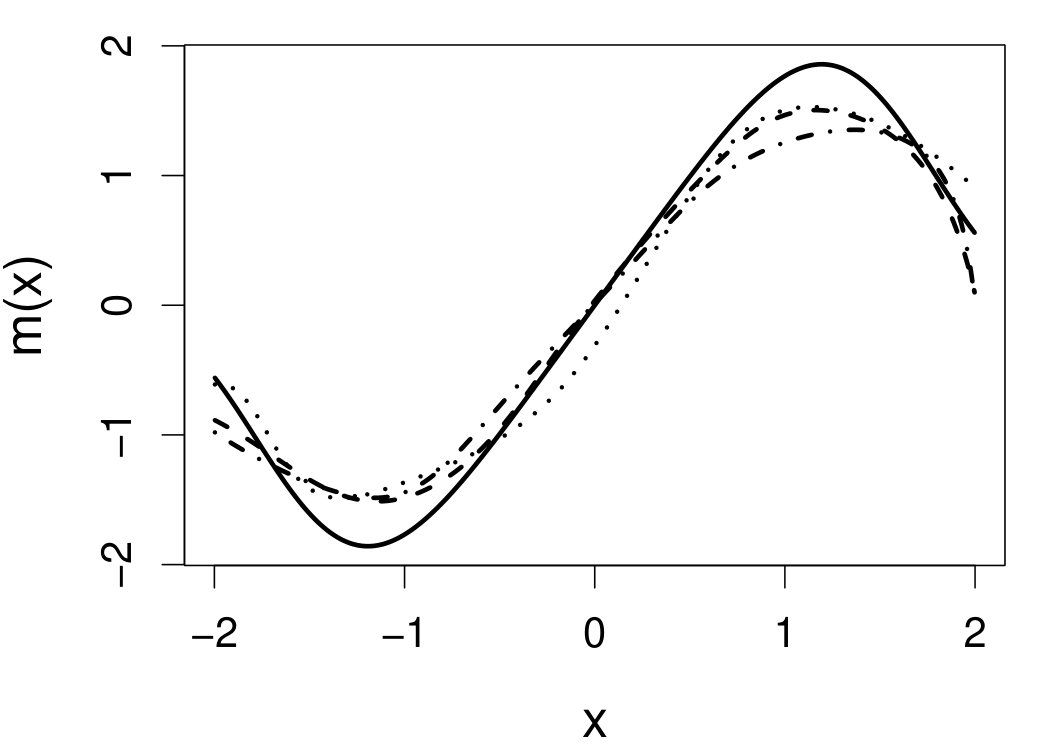 Figure 26
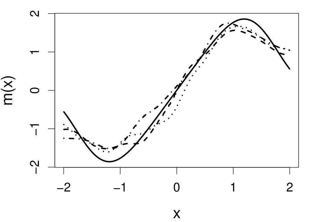 Figure 27
 Figure 28
 Figure 29
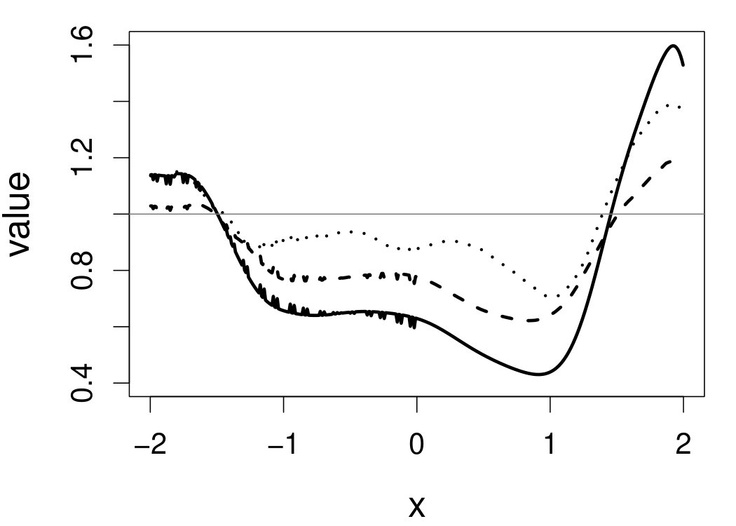 Figure 30
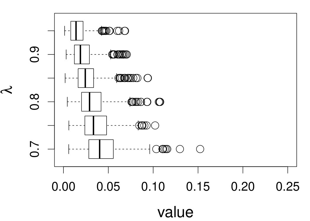 Figure 31
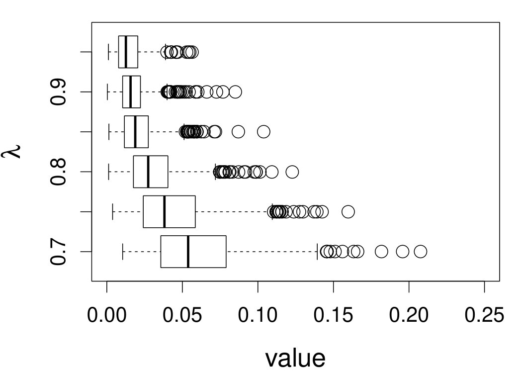 Figure 32
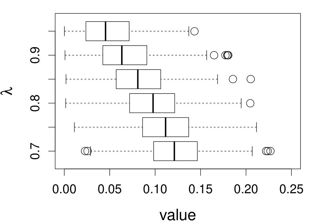 Figure 33
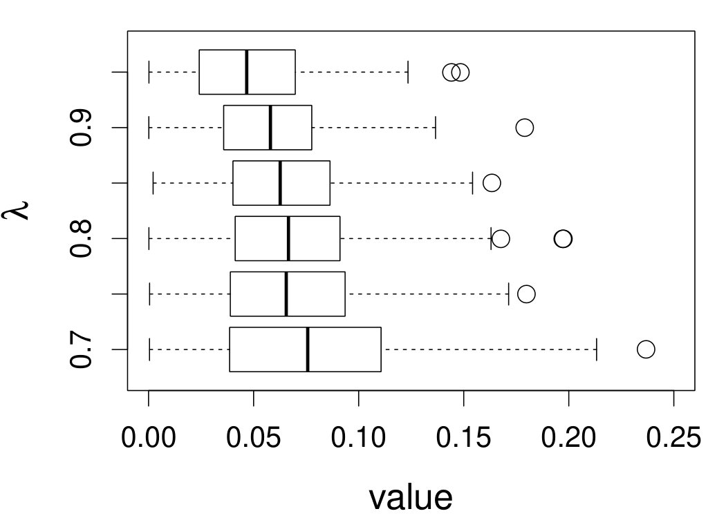 Figure 34
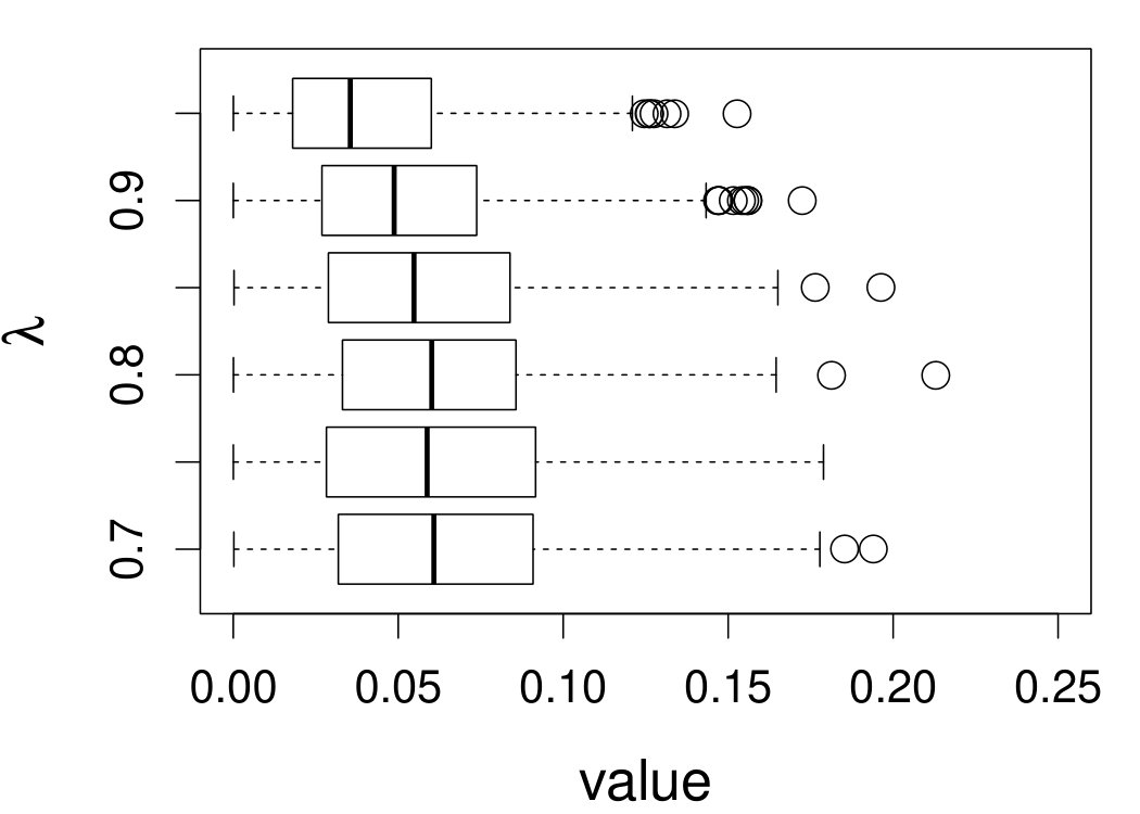 Figure 35
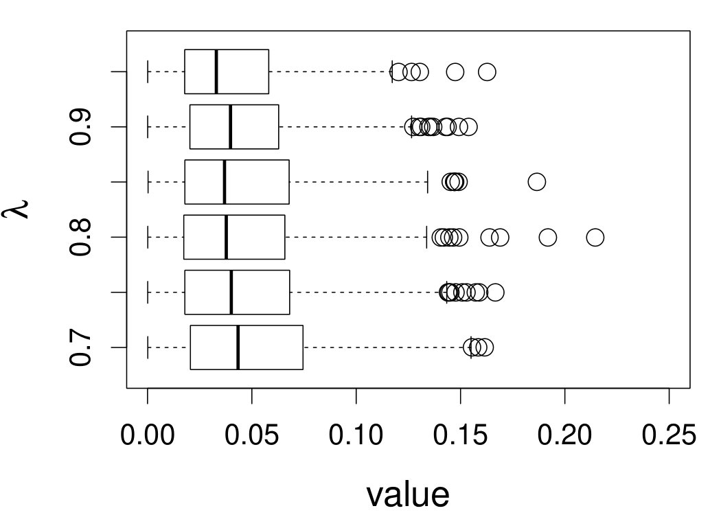 Figure 36
 Figure 37
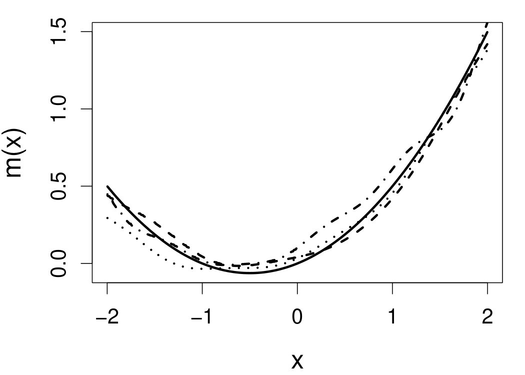 Figure 38
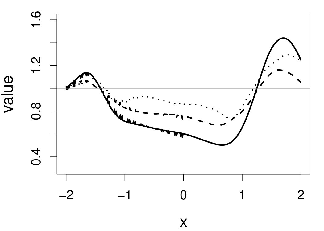 Figure 39
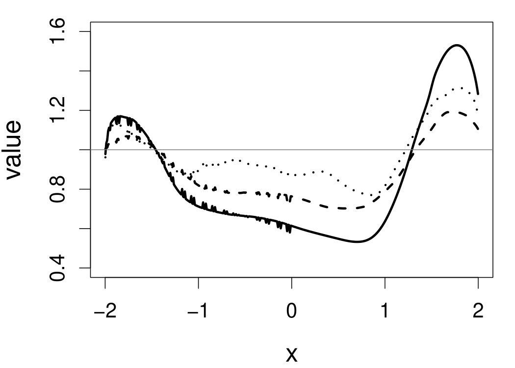 Figure 40
Peer Reviews
No public reviews on file for this paper yet. If you reviewed it on a platform where reviews are public (OpenReview, ICLR, NeurIPS, ICML), you can paste yours below so the community can read it here.
Videos
No videos yet. Explain this paper in a talk, walkthrough, or lecture? Add one.
Taxonomy
TopicsStatistical Methods and Inference · Fault Detection and Control Systems · Gaussian Processes and Bayesian Inference
An alternative local polynomial estimator for the error-in-variables problem
\nameXianzheng Huanga*∗* and Haiming Zhoub ∗Corresponding author. Email: [email protected] aDepartment of Statistics, University of South Carolina, Columbia, South Carolina, U.S.A.; bDivision of Statistics, Northern Illinois University, DeKalb, Illinois, U.S.A.
(v4.0 released June 2015)
Abstract
We consider the problem of estimating a regression function when a covariate is measured with error. Using the local polynomial estimator of Delaigle et al. (2009) as a benchmark, we propose an alternative way of solving the problem without transforming the kernel function. The asymptotic properties of the alternative estimator are rigorously studied. A detailed implementing algorithm and a computationally efficient bandwidth selection procedure are also provided. The proposed estimator is compared with the existing local polynomial estimator via extensive simulations and an application to the motorcycle crash data. The results show that the new estimator can be less biased than the existing estimator and is numerically more stable.
keywords:
convolution; deconvolution; Fourier transform; measurement error.
{classcode}
62G05; 62G08; 62G20
1 Introduction
The error-in-covariates problem has received great attention among researchers who study nonparametric inference for regression functions over the past two decades. Schennach (2004a, b) proposed an estimator of the regression function when the error-prone covariate is measured twice. Her estimator does not require a known measurement error distribution. Zwanzig (2007) proposed a local least square estimator of the regression function, assuming a uniformly distributed error-prone covariate with normal measurement error. Many more existing methods are developed under the assumption of a known measurement error distribution and an unknown true covariate distribution. Among these works, many follow the theme of deconvolution kernel pioneered in the density estimation problem in the presence of measurement error (Carroll and Hall, 1988; Stefanski and Carroll, 1990). In particular, starting from the well-known Nadaraya-Watson kernel estimator developed for error-free case (Nadaraya, 1964; Watson, 1964), Fan and Truong (1993) formulated the local constant estimator of a regression function using the deconvolution kernel technique. Generalization of this estimator to local polynomial estimators of higher orders was achieved by Delaigle et al. (2009) via introducing a complex transform of the kernel function. This transform is the key step that allows for the extension from the zero-order to a higher-order local polynomial estimator in error-in-variables problems.
In this study, we propose a new estimator motivated by an identity that relates the Fourier transform of the functions to be estimated to the Fourier transform of the counterpart naive functions. Here, a naive estimate refers to an estimate that results from replacing the unobserved true covariate one would use in the absence of measurement error with the error-contaminated observed covariate. This identity and the new estimator are presented in Section 2, following a brief review of the estimator in Delaigle et al. (2009), which we refer to as the DFC estimator henceforth. Sections 3, 4, and 5 are devoted to studying the asymptotic distribution of the new estimator. The finite sample performance of our estimator is demonstrated in comparison with the DFC estimator in Section 6. We summarize our contribution and findings, discuss some practical issues in Section 7. All appendices referenced in this article are provided in the Supplementary Materials.
2 Existing and proposed estimators
Denote by a random sample of size from a regression model with additive measurement error in the covariate specified as follow,
[TABLE]
where is the unobserved true covariate following a distribution with probability density function (pdf) f_{\hbox{\tinyX}}(x), is the measurement error, assumed to be independent of and follow a known distribution with pdf f_{\hbox{\tinyU}}(u), is the error-contaminated observed covariate following a distribution with pdf f_{\hbox{\tinyW}}(w), for . The problem of interest in this study is to estimate the regression function, , based on the observed data. The index is often suppressed in the sequel when a generic observation or random variable is referenced.
2.1 The DFC estimator
In the absence of measurement error, the well-known local polynomial estimator of order for is given by (Fan and Gijbels, 1996, Chapter 3)
[TABLE]
where \mbox{\boldmathe}_{1} is a vector with 1 in the first entry and 0 in the remaining entries,
[TABLE]
and , in which
[TABLE]
and with being a symmetric kernel function and being the bandwidth.
In the presence of measurement error, one could replace with for in the above local polynomial estimator, yielding a naive estimator of , denoted by . Clearly, is merely a sensible estimator of the naive regression function . Following the rationale behind the corrected score method (Carroll et al., 2006, Section 7.4), Delaigle et al. (2009) sought some function, denoted by , that satisfies
[TABLE]
where . The authors derived such function via solving the Fourier transform version of (4), and showed that L_{\ell}(x)=x^{-\ell}K_{\hbox{\tinyU},\ell}(x), where
[TABLE]
in which , \phi^{(\ell)}_{\hbox{\tinyK}}(t) is the -th derivative of \phi_{\hbox{\tinyK}}(t)=\int e^{itx}K(x)dx, and \phi_{\hbox{\tinyU}}(x) is the characteristic function of . Throughout this article, denotes the Fourier transform (characteristic function) of if is a function (random variable). All integrals in this article integrate over either the entire real line or a subset of it that guarantees the existence of relevant integrals, and we will make remarks on such subset whenever it is needed for clarity. The DFC estimator is given by \hat{m}_{\hbox{\tiny DFC}}(x)=\mbox{\boldmathe}_{1}^{\mathrm{\scriptscriptstyle T}}\hat{\mathbf{S}}_{n}^{-1}\hat{\mathbf{T}}_{n}, where and are similarly defined as and in (2) but with the elements in the matrices given by
[TABLE]
The transform of defined in (5) is a natural extension of the transform used in the deconvolution density estimator (Stefanski and Carroll, 1990) and the local constant estimator (Fan and Truong, 1993) of under the setting of (1). In particular, the estimator in Fan and Truong (1993) is a special case of the DFC estimator with .
2.2 The proposed estimator
Deviating from the theme of deconvolution kernel and its extension in (5), we propose a new estimator that more directly exploits the naive inference as a whole. This direct use of the naive inference is motivated by the following result proved in Delaigle (2014), m^{*}(w)f_{\hbox{\tinyW}}(w)=(mf_{\hbox{\tinyX}})*f_{\hbox{\tinyU}}(w), where (mf_{\hbox{\tinyX}})*f_{\hbox{\tinyU}}(w) is the convolution given by \int m(x)f_{\hbox{\tinyX}}(x)f_{\hbox{\tinyU}}(w-x)dx. Applying Fourier transform on both sides of this identity, one has
[TABLE]
where \phi_{m^{*}f_{\hbox{\tinyW}}}(t) is the Fourier transform of m^{*}(w)f_{\hbox{\tinyW}}(w) and \phi_{mf_{\hbox{\tinyX}}}(t) is the Fourier transform of m(x)f_{\hbox{\tinyX}}(x). Immediately following (6), by the Fourier inversion theorem, one has m(x)f_{\hbox{\tinyX}}(x)=(2\pi)^{-1}\int e^{-itx}\phi_{m^{*}f_{\hbox{\tinyW}}}(t)/\phi_{\hbox{\tinyU}}(t)dt. This motivates our local polynomial estimator of order for given by, assuming the relevant Fourier transforms well defined,
[TABLE]
where \hat{f}_{\hbox{\tinyX}}(x) is the deconvolution kernel density estimator of f_{\hbox{\tinyX}}(x) in Stefanski and Carroll (1990), and \phi_{\hat{m}^{*}\hat{f}_{\hbox{\tinyW}}}(t) is the Fourier transform of \hat{m}^{*}(w)\hat{f}_{\hbox{\tinyW}}(w), in which is the -th order local polynomial estimator of , and \hat{f}_{\hbox{\tinyW}}(w) is the regular kernel density estimator of f_{\hbox{\tinyW}}(w) (Fan and Gijbels, 1996, Section 2.7.1), i.e., the naive estimator of f_{\hbox{\tinyX}}(\cdot). Note that, although we consider a scalar covariate for notational simplicity in this article, the estimators on the right-hand side of (7) have their multivariate counterparts to account for multivariate covariates. Hence, with multivariate (inverse) Fourier transform used in (7), the proposed estimator becomes applicable to regression models with multiple covariates. Moreover, if some of these covariates are measured without error, one may reflect this in \phi_{\hbox{\tinyU}}(t) by viewing that the elements in the multivariate corresponding to the error-free covariates follow a degenerate distribution with all probability mass on zero.
By its appearance, the new estimator in (7) results from applying an integral transform similar to that in (5) on the naive product \hat{m}^{*}(\cdot)\hat{f}_{\hbox{\tinyW}}(\cdot) rather than on . It can be shown (via straightforward algebra omitted here) that, when , this new estimator is the same as the DFC estimator, both reducing to the local constant estimator in Fan and Truong (1993). Other than this special case, differs from in general.
2.3 Preamble for asymptotic analyses
The majority of the theoretical development presented in Delaigle et al. (2009) revolves around properties of the transformed kernel, K_{\hbox{\tinyU},\ell}(x), which is not surprising as K_{\hbox{\tinyU},\ell}(x) is everywhere in the building blocks of their estimator. Because of the close tie between our proposed estimator and the naive estimators, much of our theoretical development builds upon well established results for kernel-based estimators in the absence of measurement error. This can be better appreciated by interchanging the order of the two integrals in (7), assuming that \phi_{\hat{m}^{*}\hat{f}_{\hbox{\tinyW}}}(t) is compactly supported on (to allow the interchange), \hat{m}_{\hbox{\tiny HZ}}(x)\hat{f}_{\hbox{\tinyX}}(x)=\int\hat{m}^{*}(w)\hat{f}_{\hbox{\tinyW}}(w)(2\pi)^{-1}\int_{I_{t}}e^{-it(x-w)}/\phi_{\hbox{\tinyU}}(t)\,dtdw. This identity can be re-expressed more succinctly as
[TABLE]
where \mathcal{A}(w)=\hat{m}^{*}(w)\hat{f}_{\hbox{\tinyW}}(w), \mathcal{B}(x)=\hat{m}_{\hbox{\tiny HZ}}(x)\hat{f}_{\hbox{\tinyX}}(x), and D(s)=(2\pi)^{-1}\int_{I_{t}}e^{-its}/\phi_{\hbox{\tinyU}}(t)dt. Note that is a random process depending on the native estimators and \hat{f}_{\hbox{\tinyW}}(w), and results from convoluting and the non-random function . A natural question is, given the asymptotic properties of , what can be deduced from the convolution of and . More specifically, we are interested to know how the moments of compare with those of , and whether a Gaussian process on implies another Gaussian process on . These questions about random process convolution are of mathematical interest in their own rights besides being the key to understanding .
Here we provide two definitions of smoothness of a distribution (Fan, 1991a; Fan,, 1991b; Fan, 1991c) and two sets of conditions to be referenced later.
Definition 1**.**
The distribution of is ordinary smooth of order if
[TABLE]
for some positive constants and .
Definition 2**.**
The distribution of is super smooth of order if
[TABLE]
for some positive constants , , , , and .
Condition O:
For , \|\phi^{(\ell)}_{\hbox{\tinyK}}(t)\|_{\infty}<\infty and \int(|t|^{b}+|t|^{b-1})|\phi^{(\ell)}_{\hbox{\tinyK}}(t)|dt<\infty. For , \int|t|^{2b}|\phi^{(\ell_{1})}_{\hbox{\tinyK}}(t)||\phi^{(\ell_{2})}_{\hbox{\tinyK}}(t)|dt<\infty. And, \|\phi^{\prime}_{\hbox{\tinyU}}(t)\|_{\infty}<\infty.
Condition S:
For , \|\phi^{(\ell)}_{\hbox{\tinyK}}(t)\|_{\infty}<\infty, and \phi_{\hbox{\tinyK}}(t) is supported on .
In addition, we assume f_{\hbox{\tinyX}}(x)>0 and \phi_{\hbox{\tinyU}}(t) is an even function that never vanishes. We reach the convolution form in (8) under the assumption that \phi_{\hat{m}^{*}\hat{f}_{\hbox{\tinyW}}}(t) is compactly supported on , where is a region that guarantees well defined. This assumption can be easily satisfied by choosing a kernel of which the Fourier transform has a finite support. Even without this assumption the asymptotic properties presented in the following three sections still hold, although some of the proof need to be revised to use the estimator of its original form in (7). While acknowledging the overlap between the regularity conditions needed in our asymptotic analyses and those required for the DFC estimator, we also assume existence of the Fourier transform of m^{*}(\cdot)f_{\hbox{\tinyW}}(\cdot) and that of m(\cdot)f_{\hbox{\tinyX}}(\cdot) in (6). We next dissect the asymptotic bias, variance and normality of .
3 Asymptotic bias
We provide the derivations of the asymptotic bias of for in Appendix A. To better apprehend the distinction between our bias results and those of , we present a brief derivation of the bias when in this section.
3.1 Dominating bias when
Define , for . Let A(w)=m^{*}(w)f_{\hbox{\tinyW}}(w) and B(x)=m(x)f_{\hbox{\tinyX}}(x) be the non-random counterparts of and in (8), respectively. Then, like (8), we have .
By Theorem 2.1 in Stefanski and Carroll (1990), the deconvolution density estimator \hat{f}_{\hbox{\tinyX}}(x) is a consistent estimator of f_{\hbox{\tinyX}}(x). Noting that \hat{f}_{\hbox{\tinyX}}(x)/f_{\hbox{\tinyX}}(x) converges to one in probability, we derive the dominating bias via elaborating E[\{\hat{m}_{\hbox{\tiny HZ}}(x)-m(x)\}\hat{f}_{\hbox{\tinyX}}(x)/f_{\hbox{\tinyX}}(x)|\mathbb{W}], which is equal to
[TABLE]
where , and
[TABLE]
To derive in (9), we invoke the following two results for kernel-based estimators in the absence of measurement error (Fan and Gijbels, 1996, Chapter 3),
[TABLE]
Following these results, one can show that
[TABLE]
where M(w)=m^{*}(w)f^{(2)}_{\hbox{\tinyW}}(w)+m^{*(2)}(w)f_{\hbox{\tinyW}}(w). Then, assuming interchangeability of expectation and integration, (8) and (11) imply
[TABLE]
Finally, by (10) and (12), (9) reduces to
[TABLE]
which reveals the dominating bias of of order .
Different from Delaigle et al. (2009), we directly use the existing results associated with estimators in the absence of measurement error for deriving the asymptotic bias.
3.2 Comparison with the bias of the DFC estimator
By Theorem 3.2 in Delaigle et al. (2009), the dominating bias of is the same as that of , which is when . To make the comparison of dominating bias more tractable, we consider regression functions in the form of a polynomial of order , . Furthermore, we set and , resulting in a reliability ratio (Carroll et al., 2006, Section 3.2.1) of .
Under this setting, the dominating bias in (13) can be derived explicitly. Instead of directly comparing the dominating bias associated with the two estimators, we focus on studying the number of ’s at which each dominating bias is zero. Note that is a polynomial of order provided that , and thus the dominating bias of is zero at no more than ’s. In contrast, we show in Appendix A that the dominating bias in (13) reduces to a polynomial of order , suggesting that the dominating bias of can be zero at ’s. Suppose that the bias of each estimator is continuous in , which is a realistic assumption in many applications. Then having two more roots to the equation, , for indicates that the proposed estimator can have two more regions in the support of within which is less biased than , where each region is a neighborhood of some root. For example, when , clearly the dominating bias of can never be zero. It is shown in Appendix A that, the dominating bias of is zero at the roots of the equation . With , one can easily show that this quadratic equation has two roots.
4 Asymptotic variance
Because
[TABLE]
we focus on deriving in order to study the asymptotic variance of . Detailed derivations are provided in Appendix B, which consists of five steps. In what follows, we provide a sketch of the derivations, where we highlight the connection between our results and the counterpart results in the absence of measurement error, and how our derivations differ from and relate to those in Delaigle et al. (2009).
4.1 Derivations of
First, we deduce from (8) that can be formulated as an iterative convolution of the covariance of as follows,
[TABLE]
Since \hat{f}_{\hbox{\tinyW}}(w)/f_{\hbox{\tinyW}}(w) converges to 1 in probability under regularity conditions,
[TABLE]
Second, we view as a weighted least squares estimator (Fan and Gijbels, 1996, page 58), and show that
[TABLE]
where \mbox{\boldmath\Sigma}_{12}=\textrm{diag}\{K_{h}(W_{1}-w_{1})K_{h}(W_{1}-w_{2})\nu^{2}(W_{1}),\ldots,K_{h}(W_{n}-w_{1})K_{h}(W_{n}-w_{2})\nu^{2}(W_{n})\}, , and, for , ,
[TABLE]
Then we approximate the random quantities on the right hand side of (17) to establish that
[TABLE]
where and \mathbf{S}^{*}_{\hbox{\tinyW},h}=(\xi_{\ell_{1},\ell_{2}}((w_{1}-w_{2})/2,h))_{0\leq\ell_{1},\ell_{2}\leq p}, in which, for ,
[TABLE]
The result in (LABEL:eq:covmm2) is a counterpart result of , where (Fan and Gijbels, 1996, equation (3.7)).
Third, substituting (LABEL:eq:covmm2) in (16) gives
[TABLE]
where \gamma(w)=\nu^{2}(w)f_{\hbox{\tinyW}}(w). And plugging (20) in (15) yields
[TABLE]
Note that, among the matrices in (LABEL:eq:varB2), only \mathbf{S}^{*}_{\hbox{\tinyW},h} depends on and , of which the entries are in (19).
The fourth step is to derive
[TABLE]
which is equal to
[TABLE]
Define \kappa_{\ell_{1},\ell_{2}}(h)=\int K_{\hbox{\tinyU},\ell_{1}}(v)K_{\hbox{\tinyU},\ell_{2}}(v)\,dv to highlight the dependence of this integral on (since K_{\hbox{\tinyU},\ell}(v) depends on according to (5)), and define matrix . To this end, we can conclude that, by (LABEL:eq:varB2) and (23),
[TABLE]
This is where the path of our derivations meets that of Delaigle et al. (2009), as now we need to incorporate the properties of as (and thus ), for an ordinary smooth and for a super smooth , respectively. These properties are thoroughly studied in Delaigle et al. (2009) and summarized in their Lemmas B.4, B.6, B.9, which are restated in Appendix B for completeness. Equipped with these lemmas, we are ready to move on to the fifth step of the derivations.
By Lemma B.4, for an ordinary smooth , under Condition O, as , where
[TABLE]
in which and are constants in Definition 1. Define , then , and thus (24) implies (25) in Theorem 4.1 below. For a super smooth , by Lemma B.9, under Condition S, , where , , and are constants in Definition 2, and is some generic non-negative finite constant appearing in Lemma B.8 in Delaigle et al. (2009). This leads to (26) in Theorem 4.1 below, which serves as a recap of our findings in this subsection.
Theorem 4.1**.**
When is ordinary smooth of order , under Condition O, if , then
[TABLE]
When is super smooth of order , under Condition S, if , then is bounded from above by
[TABLE]
4.2 Comparison with the variance of the DFC estimator
By Theorem 3.1 in Delaigle et al. (2009), when the distribution of is ordinary smooth, under Condition O, if , then
[TABLE]
where . Note that the asymptotic variance results in Theorem 4.1, as well as the asymptotic bias results in Section 3, are conditional on whereas (27) is an unconditional variance. The conditional arguments in our moment analysis originate from the direct use of asymptotic moments of the local polynomial estimator of a regression function in the absence of measurement error, which are conditional moments given (Ruppert and Wand, 1994). As pointed out in Ruppert and Wand (1994, Remark 1, page 1351), because the dominating terms in these conditional moments are free of , they still have the interpretation of unconditional dominating moments. Once this is clear, one can see that the difference between the dominating variance in (27) and that in (25) lies in the distinction between (\tau^{2}f_{\hbox{\tinyX}})*f_{\hbox{\tinyU}}(x) and . It is shown in Appendix B that \gamma(x)=(\tau^{2}f_{\hbox{\tinyX}})*f_{\hbox{\tinyU}}(x)+f_{\hbox{\tinyW}}(x)\textrm{Var}\{m(X)|W=x\}\geq(\tau^{2}f_{\hbox{\tinyX}})*f_{\hbox{\tinyU}}(x). Hence, for an ordinary smooth , the dominating variance of is greater than or equal to that of . In Section 6, we will see how this large sample comparison takes effect in the comparison of finite sample variances associated with the two estimators.
5 Asymptotic normality
Under the conditions stated in Theorem 4.1, we show the asymptotic normality of in Appendix C. The logic behind the proof is similar to that in Delaigle et al. (2009). More specifically, we first approximate via an average, , where is a set of independent and identically distributed (i.i.d.) random variables at each fixed . Then we show that, for some positive constant ,
[TABLE]
which is a sufficient condition for
[TABLE]
This in turn leads to the asymptotic normality of , and further suggests the asymptotic normality of .
To this end, we have answered the questions raised in Section 2.3 regarding the properties of a random process resulting from the convolution of another random process and the non-random function . We now see that the first two moments of are closely related to the the first two moments of via similar convolutions. Also, if is asymptotically Gaussian, then under mild regularity conditions, is also asymptotically Gaussian, and many of these conditions can be satisfied by choosing an appropriate kernel function in .
6 Implementation and finite sample performance
After a thorough investigation of asymptotic properties of the proposed estimator, we are now in the position to look into its finite sample performance. By the construction of , we need to evaluate continuous Fourier transforms (CFT) and inverse CFTs. In this section we first describe the algorithm for these evaluations, then discuss bandwidth selection. Finally, we present experiments to compare our estimator with the DFC estimator under four settings where we simulate data from the true models with our design of , and under another setting where error-prone data are simulated from a motorcycle-crash data set with the underlying unknown.
6.1 Numerical evaluations
For an integrable function that maps the real line onto the complex space, , define the CFT of as
[TABLE]
In our study, we first approximate the CFT via a discrete Fourier transform (DFT), then we use the fast Fourier transform algorithm (FFT, Bailey and Swarztrauber, 1994) to evaluate the corresponding DFT. For a sequence of complex values , the DFT is defined as , for , which can be easily evaluated using FFT in standard statistical software. The approximation of CFT using DFT is sketched next.
To prepare for the approximation, one first specifies a sequence of input values and then specifies a sequence of output values accordingly. More specifically, let be the input values for the CFT, where is an even integer, is the increment, and is chosen such that (28) can be well approximated by . With the input values specified, the corresponding output values are , where . With the input and output values ready, we approximate the CFT as follows, for ,
[TABLE]
This approximation converges to the truth very rapidly provided that the Fourier coefficients of rapidly decrease (Davis and Rabinowitz, 1984). The values of and determine the resolution of the input and output results, respectively. Comparable resolutions in and are typically desired, which can be achieved by setting . A larger tends to yield a more accurate approximation of the CFT. Bailey and Swarztrauber (1994) computed the CFT of the standard normal density function using and achieved the root-mean-squared error of order . In the simulations presented in this article, we set , resulting in and . In additional simulation studies where we used a larger , we found the results essentially unchanged. This algorithm can be similarly applied to approximate the inverse CFT.
6.2 Bandwidth selection
It has been well acknowledged that the choice of bandwidth is crucial in kernel-based nonparametric estimation. In our study, we adopt the method of cross-validation (CV) in conjunction with simulation extrapolation (SIMEX, Carroll et al., 2006, Chapter 5) as proposed by Delaigle and Hall (2008). To implement this method, one first randomly divides the observed data, , into subsamples of (nearly) equal size. Denote by the th subsample, and the set of subject indices corresponding to the observations in , for . Then one carries out two rounds of -fold cross validation using further contaminated data. In the first round, one generates further contaminated data according to , for and , where are i.i.d. according to f_{\hbox{\tinyU}}(u). Viewing as the “unobserved true” covariate values, and as the target regression function to be estimated using the “observed” data, , for , one may use the proposed method to estimate . Denote this estimator by . Now one carries out the -fold cross validation to choose a bandwidth for estimating that minimizes
[TABLE]
where is the estimate computed using the further contaminated data excluding , for , and is a suitable weight function. Define . In the second round of -fold cross validation, another set of further contaminated data is produced according to , where are i.i.d. according to f_{\hbox{\tinyU}}(u), for and , also independent of . Similar to the first round, one views as the “unobserved true” covariate values, and considers estimating another target regression function using the proposed method based on the “observed” data , for . Denote this estimator by . To select a bandwidth for estimating , one minimizes the following criterion with respect to ,
[TABLE]
where is the estimate computed using the data excluding , for . Define . Finally, one sets as the bandwidth used in for estimating based on the original observed data .
This bandwidth selection procedure can be computationally cumbersome because, first, in search of and , one needs to evaluate and on a fine grid of candidate bandwidths; second, as recommended in most SIMEX applications, one needs a not too small in order to control the Monte Carlo variability when generating further contaminated data. To reduce the computational burden, we propose a procedure to refine the search region of . Take the first round of cross validation described above as an example. Recall that, during this round, is viewed as the unobserved true covariate values whereas is the error-contaminated version of the true covariate values. To narrow down the search region of when minimizing , we first find an initial bandwidth, . In particular, we obtain by minimizing the following approximated mean integrated squared error (MISE) for the deconvolution kernel density estimator of f_{\hbox{\tinyW}}(w) using (Stefanski and Carroll, 1990),
[TABLE]
where \int\{f^{\prime\prime}_{\hbox{\tinyW}}(w)\}^{2}dw can be easily estimated using . After is found, we search for across grid points within . This strategy is motivated by the theoretical finding that the deconvolution kernel regression estimators have the same optimal rates as the deconvolution kernel density estimators. In our extensive trial-and-error simulation experiments under the model settings described in Section 6.3, we considered a wider search region that encompasses , and we observed all selected indeed fell in the above refined search region. Similarly, in the second round of cross validation where we search for across grid points within , where is chosen by minimizing (29), but, different from the first round, now \int\{f^{\prime\prime}_{\hbox{\tinyW}}(w)\}^{2}dw there is replaced by \int\{f^{\prime\prime}_{\hbox{\tinyW^{*}}}(w)\}^{2}dw, which can be easily estimated using .
One may legitimately question our choice of the multiplicative factors, 0.2 and 2, in the recommended refined search region of . For a given application, the safe and conservative way to choose usually involves some trial-and-error. If the optimal found within this refined region is too close to one of the boundaries, one may consider pushing that end of the region out slightly and adjusting the search region accordingly. Using the refined search region of at each round of cross validation, we also observe in simulations that one can even use a much smaller without noticeably compromising the quality of . This refined bandwidth selection procedure and the algorithm for approximating CFT and inverse CFT described in Section 6.1 are implemented in an R package called lpme created and maintained by the second author, which provides both and .
6.3 Simulation study
In the simulation experiments, we compare realizations of and (with ) obtained under the following four model configurations:
- (C1)
, where , , X_{1}\sim f_{\hbox{\tinyX_{1}}}(x)=0.1875x^{2}I_{[-2,2]}(x), , and . 2. (C2)
, where , , and . 3. (C3)
, where , , and . 4. (C4)
, where , , and .
Among these configurations, (C1) is considered in Delaigle et al. (2009); (C2) creates a scenario where the dominating bias of never vanishes since is a second-order polynomial; (C3), with being a higher order polynomial, results in zero dominating bias for within the support of at ; and (C4) has out of the polynomial family yet it can be expanded as a polynomial of infinite order. Besides the model configuration, we also vary the reliability ratio from 0.7 to 0.95 at increments of 0.05 when generating . Under (C2), although the measurement errors are simulated from a normal distribution, we computed the estimates of assuming a normal first, and then we repeated the estimation assuming a Laplace . This exercise allows us to observe the effects of a misspecified distribution for on the estimates. Under each simulation setting, Monte Carol (MC) replicates of sample size are generated from the true model of . For both estimation methods, we used the kernel of which the Fourier transform is given by \phi_{\hbox{\tinyK}}(t)=(1-t^{2})^{8}I_{[-1,1]}(t).
Denote by one of the two estimates under comparison generically. For the majority of the simulation experiments, in order to mitigate the confounding effect of a data-driven bandwidth selection method on the quality of , we computed using the theoretical optimal bandwidth obtained via minimizing an approximate of the integrated squared error (ISE), , where is the interval of the true covariate value of interest. This approximated is given by , where is the partition resolution, is the largest integer no greater than , and , for . For a small portion of the presented simulation experiments, we used the CV-SIMEX bandwidth selection strategy described in Section 6.2 to select a bandwidth for each of the two estimators. Note that, when choosing a bandwidth for , one should change and in Section 6.2 to the counterpart estimates and , respectively.
We compare the performance of and with regard to the quality of the entire regression curve estimation over , as well as the quality of the estimation of at individual ’s. The quantity used to monitor the overall regression curve estimation is the approximated ISE. The quantities used to assess the quality of at a particular point are based on the pointwise absolute error (PAE), . Specifically, we compute the following three summary statistics: first, the pointwise mean absolute error ratio (PmAER) defined by
[TABLE]
second, the pointwise standard deviation of absolute error ratio (PsdAER) defined by
[TABLE]
and third, the pointwise mean squared error ratio (PMSER) defined by
[TABLE]
These quantities are presented in Figures 1–4 for (C1)–(C4), respectively. Figure 5 shows the counterpart results of Figure 2 under (C2) when it is (incorrectly) assumed that follows a Laplace distribution. These five figures depict results obtained when the theoretical optimal is used. Lastly, Figure 6 is the counterpart of Figure 4 under (C4) with chosen by the CV-SIMEX bandwidth selection procedure with and . Very similar performance of the two estimates is observed when larger values of or are used in this round of experiment.
When the theoretical optimal bandwidth is used, as in Figures 1–5, outperforms over the majority region of each considered range of in regard to both accuracy and precision. Even though it is shown in Section 4.2 that the dominating variance of is higher than that of when the distribution of is ordinary smooth (e.g., a Laplace distribution), this large sample trend does not take effect for the majority region of in these finite sample experiments. The regions where performs better than in regard to bias, variance, and MSE are usually neighborhoods of the inflection points of . For instance, under (C3) (see panel (i) in Figure 3), is less biased than at the small neighborhoods of . It is worth pointing out that the gain in accuracy and precision from our estimator compared to the DFC estimator is especially promising at the boundary of in (C3) and (C4) (see panels (c), (f), and (i) in Figures 3 and 4). In both cases, data points uniformly distribute over the domain of . Different from (C3) and (C4), in (C1), there are more data points near the boundaries than elsewhere in the domain. Excluding (C2) (since the plotted range of in Figures 2 and 5 is not the entire observed range), (C1) is the only case among all considered cases here that outperforms near the boundaries in terms of bias. However, is still substantially less variable, and its MSE is lower than that of the competing estimator (see panels (c), (f), and (i) of Figure 1). Finally, contrasting Figure 2 and Figure 5, one can see that both estimators are fairly robust to the misspecification of the measurement error distribution.
When the bandwidth is chosen by the refined CV-SIMEX method, as in Figure 6, both estimates become more variable, with our estimates better than the DFC estimates over most of the 500 MC replicates. As mentioned earlier, increasing to a larger value does not substantially change our estimate. More importantly, using a smaller than ten affects our estimator far less than it affects the DFC estimator.
6.4 Motorcycle data
We now apply the two estimation methods to error-contaminated data sets created based on the motorcycle crash data from a simulated motorcycle crash designed to test crash helmets (available under R library MASS). The original data set consists of 133 measurements of head acceleration measured in standard gravity acceleration (gs) at various times in milliseconds after impact. It is of interest to estimate the underlying head acceleration, , as a function of time after impact, . Having the error-free data in this example allows us to have a reference estimate of the regression function with which the estimates based on error-prone data can be compared.
Based on the original data, we first obtain the local linear estimate of , denoted by , using the R function locpol in the locpol package, with the bandwidth chosen by cross validation (Wang and Jones, 1995) implemented by function regCVBwSelC in the same R package. Compared to the fitted curves using error-prone data, the can be viewed as the “ideal” estimate in the sense that one cannot do better than this with error-contaminated data. We use this ideal curve as the reference curve in our follow-up experiments, where we contaminate with simulated independent Laplace measurement errors to achieve different levels of reliability ratio . At each level of , we use the error-contaminated data to estimate the acceleration curve using the two estimation methods, both assuming Laplace . This experiment of curve estimation is repeated 500 times at each level of . We obtained very similar results when we contaminated with simulated normal while assuming Laplace for estimations.
Figure 7 depicts the results, including boxplots of ISE at each level, the fitted curves for selected according to quantiles of ISE when the approximated theoretical optimal is used, and the counterpart fitted curves when the refined CV-SIMEX method is used to select with and . Using the ideal estimate as the “truth,” our estimate appears to be less biased and less variable at all considered levels of error contamination than the DFC estimate. When the refined CV-SIMEX method is used to select , our estimator suffers less numerical instability compared to the competing method.
7 Discussion
In this study we proposed a local polynomial estimator of the regression function when the covariate is measured with error. The proposed estimator makes direct use of the naive inference, leading to relatively more transparent connections between the properties of the proposed estimator and those of the inference from error-free data. We rigorously derived the asymptotic properties of the proposed estimator in comparison with the estimator proposed by Delaigle et al. (2009). Under very similar regularity conditions, besides the asymptotic normality that both estimators possess, the asymptotic bias and variance of these estimators are carefully compared. Theoretical evidence suggests that the new estimator can be less biased than the competing estimator. Results from extensive simulation study also support this finding.
To implement the proposed method, we thoughtfully refined the CV-SIMEX bandwidth selection method proposed by Delaigle and Hall (2008) to narrow the search region of , which in turn allows us to use a much smaller in the SIMEX implementation without noticeable loss in accuracy. This refinement greatly reduces the computational burden for the otherwise intrinsically cumbersome bandwidth selection procedure.
In our simulation studies, how the proposed estimator and the DFC estimator compare at the boundary of the support of depends on the distribution of . Even though the proposed estimator appears to suffer less numerical instability when the refined CV-SIMEX method is used to select , it can still be rather challenging to estimate the curve near the boundary. The properties of our estimator near the boundary deserve further investigation, which may lead to ways to improve its behavior near the boundary. Besides the generalization of the proposed method pointed out earlier in Section 2.2 to allow multiple covariates, one can also follow the construction of the proposed estimator in (7) to obtain non-naive estimators of by starting with a parametric naive estimator . For instance, one may naively fit a polynomial regression function to obtain , then use it in (7) to achieve a non-naive estimator of that is not completely nonparametric. However, the obtained estimator of is usually not of the same functional form as . If one wishes to fit a polynomial regression function accounting for measurement error, the method proposed by Zavala et al. (2007) is a more appealing approach than our proposed nonparametric approach.
The measurement error distribution is assumed be known in the simulation study presented in Section 6.3, where in one case the distribution is misspecified as a Laplace distribution, and we apprehend little influence of such misspecification on the proposed estimator. This robustness phenomenon is also pointed out in Delaigle et al. (2009) for the DFC estimator, and is discussed in Meister (2004) and Delaigle (2008). Taking advantage of this robustness feature, when the measurement error distribution is unknown, we recommend using the mean-zero Laplace characteristic function, \phi_{\hbox{\tinyU}}(t)=1/\{1+(\sigma^{2}_{u}/2)t^{2}\} in the estimator, where can be trivially and consistently estimated by equation (4.3) in Carroll et al. (2006) when repeated measures of each are available. We implement this recommended strategy for the four cases considered in Section 6.3 and observe very similar results as those shown in Figures 1–5. In particular, we generate two replicate measures, , where ’s are i.i.d. with variance , for , . Then we define , for , as the observed covariate values used in and , where the associated measurement error variance is . Following equation (4.3) in Carroll et al. (2006), we estimate via . Figure 8 shows the counterpart results of those shown in Figure 5, from which we can see that using an estimated variance in the misspecified \phi_{\hbox{\tinyU}}(t) does not affect the estimates noticeably. Plots parallel to Figures 1, 3, and 4, which show estimates obtained using the same strategy under the other three cases, are given in Appendix D.
Alternatively, one may follow the approach proposed by Delaigle et al. (2008) to estimate \phi_{\hbox{\tinyU}}(t) when repeated measures are available, which we also implement in the four cases considered in Section 6.3 using the aforementioned simulated repeated measures. Although this approach frees one from assuming a specific distribution for and estimating , the resultant estimates are mostly inferior to the estimates resulting from an assumed Laplace with estimated. Figure 9 shows the comparison between these two treatments of \phi_{\hbox{\tinyU}}(t) in our proposed estimator in regard to bias, variability, and MSE. In the three ratios, PmAER, PsdAER, and PMSER, depicted in Figure 9, the estimate in the numerators is our estimate assuming Laplace with an estimated , and the estimate in the denominator is our estimate with the estimated \phi_{\hbox{\tinyU}}(t). The comparison clearly shows that there is no gain from estimating \phi_{\hbox{\tinyU}}(t) instead of simply assuming a Laplace with estimated. Obviously, neither nor \phi_{\hbox{\tinyU}}(t) is identifiable when one does not have repeated measures or other forms of external data that allow one estimate the measurement error distribution. In this case, one can carry out sensitivity analysis with varying over a range of practical interest.
Supplemental materials
The supplement to this article contains Appendices A–D referenced in Sections 3, 4, 5, and 7.
Acknowledgments
The authors express sincere thanks to the Editor, the Associate Editor and an anonymous referee for their constructive and valuable suggestions on this article, which have led to significant improvements.
Disclosure statement
No potential conflict of interest was reported by the authors.
Funding
The first author gratefully acknowledges support from the NSF under grant number DMS-1006222.
The reference list from the paper itself. Each links out to its DOI / PubMed record.
- 1Bailey and Swarztrauber (1994) Bailey, D. and Swarztrauber, P. (1994), ‘A fast method for the numerical evaluation of continuous Fourier and Laplace transforms’, SIAM Journal on Scientific Computing , 15, 1105–1110.
- 2Carroll and Hall (1988) Carroll, R. and Hall, P. (1988), ‘Optimal rates of convergence for deconvoluting a density’, Journal of the American Statistical Association , 83, 1184–1186.
- 3Carroll et al. (2006) Carroll, R., Ruppert, D., Stefanski, L. A., Crainiceanu, C. M. (2006), Measurement error in nonlinear models: A model perspective (2nd ed.), Chapman & Hall/CRC. Boca Raton, FL.
- 4Davis and Rabinowitz (1984) Davis, P. J. and Rabinowitz, P. (1984), Methods of Numerical Integration . Academic Press.
- 5Delaigle (2008) Delaigle, A. (2008), ‘An alternative view of the deconvolution problem’, Statistica Sinica , 18, 1025-1045.
- 6Delaigle (2014) Delaigle, A. (2014), ‘Nonparametric kernel methods with errors-in-variables: constructing estimators, computing them, and avoiding common mistakes’, Australian & New Zealand Journal of Statistics , 56, 105–124.
- 7Delaigle et al. (2009) Delaigle, A., Fan, J., and Carroll, R. (2009), ‘A design-adaptive local polynomial estimator for the error-in-variables problem’, Journal of the American Statistical Association , 104, 348–359.
- 8Delaigle and Hall (2008) Delaigle, A. and Hall, P. (2008), ‘Using SIMEX for smoothing-parameter choice in errors-in-variables problems’, Journal of the American Statistical Association , 103, 280-287.