Influence of the number of predecessors in interaction within acceleration-based flow models
Antoine Tordeux, Mohcine Chraibi, Andreas Schadschneider, Armin, Seyfried

TL;DR
This paper analyzes how the number of predecessors in acceleration-based flow models affects stability, revealing non-monotonic relations and providing conditions for stability in microscopic pedestrian and car-following models.
Contribution
It introduces a stability analysis considering multiple predecessors and uncovers unexpected non-monotonic effects on stability in flow models.
Findings
Stability depends on small relaxation times.
Non-monotonic relation between number of predecessors and stability.
General conditions for linear stability on ring geometries.
Abstract
In this paper, the stability of the uniform solutions is analysed for microscopic flow models in interaction with predecessors. We calculate general conditions for the linear stability on the ring geometry and explore the results with particular pedestrian and car-following models based on relaxation processes. The uniform solutions are stable if the relaxation times are sufficiently small. The analysis is focused on the relevance of the number of predecessors in the dynamics. Unexpected non-monotonic relations between and the stability are presented.
Click any figure to enlarge with its caption.
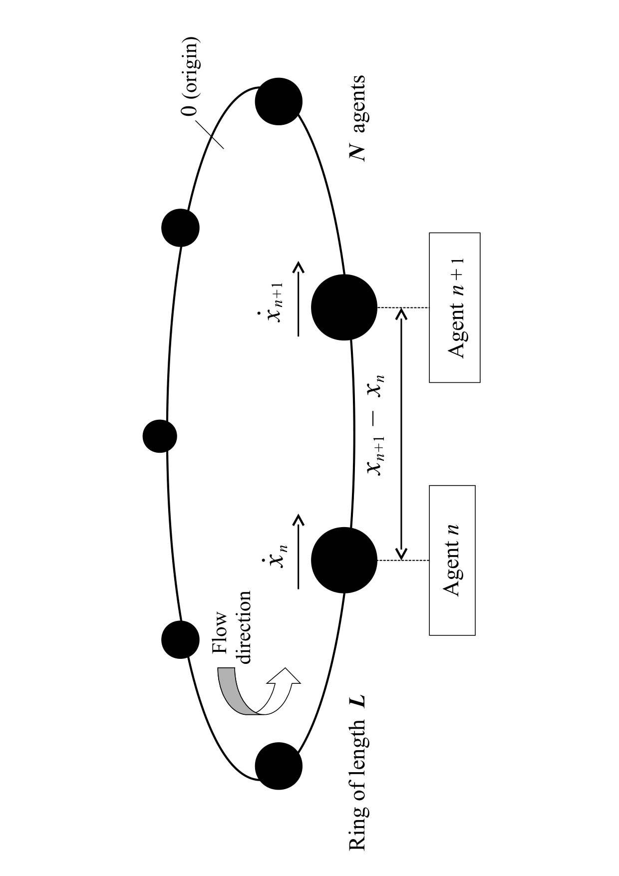 Figure 0
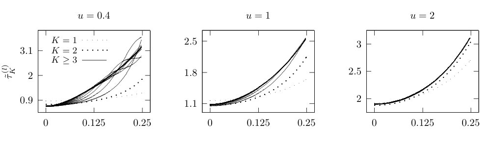 Figure 1
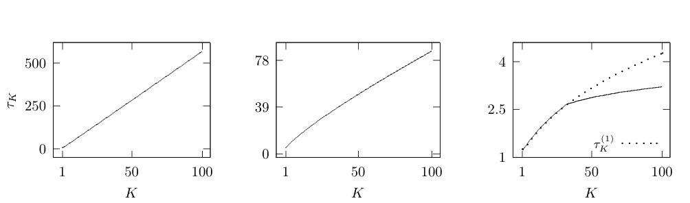 Figure 10
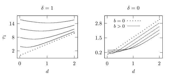 Figure 11
 Figure 12
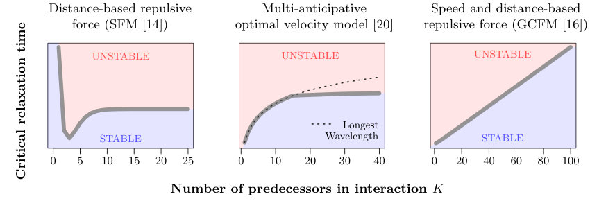 Figure 13
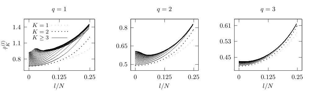 Figure 2
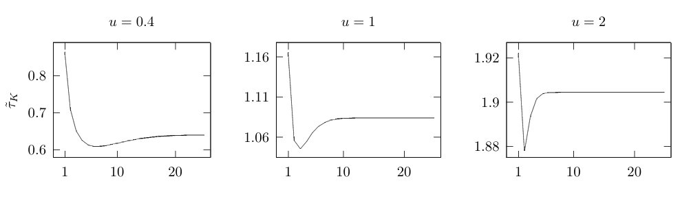 Figure 3
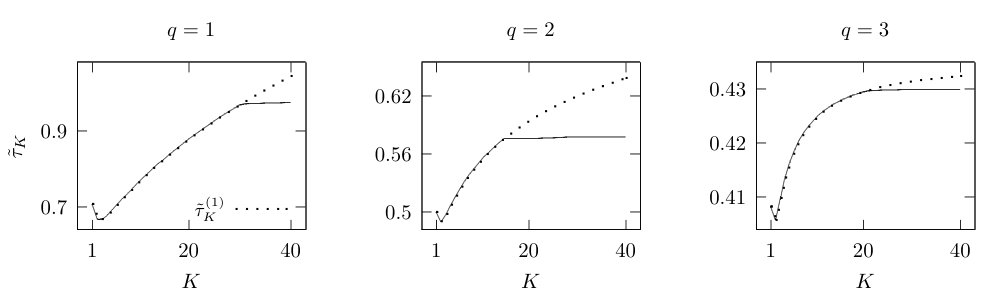 Figure 4
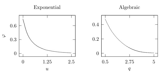 Figure 5
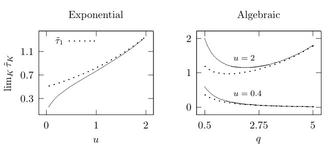 Figure 6
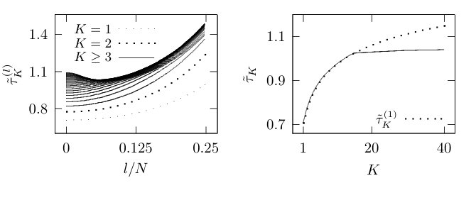 Figure 7
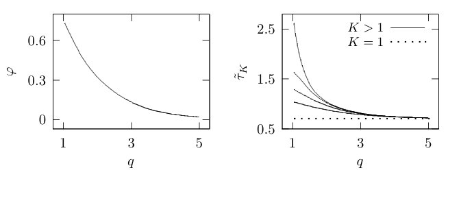 Figure 8
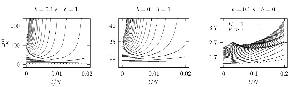 Figure 9
| Models | Range | Positive equil. speed | Stability for | Cut-off radius | Unstable wave |
|---|---|---|---|---|---|
| Exponential | Short | Bounded, | Implicit | Longest | |
| SFM [14] | non-monotonic | ||||
| Algebraic | Long | Bounded, | Implicit | Characteristic | |
| [15, 32] | if | non-monotonic | for large | ||
| OV [20] | Long | Given by | Unbounded, | To be | Characteristic |
| non-decreasing | calibrated | for large | |||
| Short | Given by | Bounded, | Implicit | Characteristic | |
| non-decreasing | for large | ||||
| GCF [16] | Long | Solution of | Unbounded, | To be | Longest |
| degree polynomials | non-decreasing | calibrated | |||
| Long | Solution of | Bounded, | Implicit | Characteristic | |
| degree polynomials | non-decreasing | for large |
Peer Reviews
No public reviews on file for this paper yet. If you reviewed it on a platform where reviews are public (OpenReview, ICLR, NeurIPS, ICML), you can paste yours below so the community can read it here.
Videos
No videos yet. Explain this paper in a talk, walkthrough, or lecture? Add one.
Influence of the number of predecessors in interaction
within acceleration-based flow models
Antoine Tordeux1,2,111Corresponding author. Email address: [email protected] , Mohcine Chraibi1, Andreas Schadschneider3 and Armin Seyfried1,2
Institute for Advanced Simulation, Forschungszentrum Jülich GmbH, Germany
Computer Simulation for Fire Safety and Pedestrian Traffic, Bergische Universität Wuppertal, Germany
Institut für Theoretische Physik, Universität zu Köln, Germany
Abstract
In this paper, the stability of the uniform solutions is analysed for microscopic flow models in interaction with predecessors. We calculate general conditions for the linear stability on the ring geometry and explore the results with particular pedestrian and car-following models based on relaxation processes. The uniform solutions are stable if the relaxation times are sufficiently small. However the stability condition strongly depends on the type of models. The analysis is focused on the relevance of the number of predecessors in the dynamics. Unexpected non-monotonic relations between and the stability are presented. Classes of models for which increasing the number of predecessors in interaction does not yield an improvement of the stability, or for which the stability condition converges as increases (i.e. implicit finite interaction range) are identified. Furthermore, we point out that increasing the interaction range tends to generate characteristic wavelengths in the system when unstable.
Keywords: Microscopic flow models, number of neighbors in interaction, homogeneous solution, linear stability analysis
1 Introduction
1.1 Context
Self-driven many-body systems are frequently used to model pedestrian or road traffic streams [1, 2, 3]. Continuous speed and acceleration models are defined with systems of ordinary, stochastic or delayed differential equations. They admit the uniform configurations (where all the spacing and speed are constant and equal) as a stationary solution. The stability analysis allows to determine conditions on the parameters for which perturbations around the uniform solution disappear (see for instance [4, 5, 6]). Real observations of pedestrian or vehicle streams present non-homogeneous configurations, with propagation of so-called stop-and-go waves for congested density levels [7, 8]. Therefore, realistic models should have unstable uniform solutions [9].
Traffic flow models can be microscopic, mesoscopic (kinetic), or macroscopic [6]. Microscopic models describe the individual trajectories in Lagrangian coordinates. They are usually called self-driven or motorized particle systems. Microscopic models are used since the 1950’s for traffic flow modelling in 1D (see for instance [10, 11, 12]), and since the 1970’s for pedestrians in 2D (see, e.g., [13, 14, 15, 16]). Speed-based models refer to as models of the first order while acceleration-based models generally refer to as second order models, or again force-based models for pedestrian dynamics in analogy to the Newtonian mechanic. The models are investigated theoretically or as simulation tools, notably to understand the formation and propagation of stop-and-go waves [5, 17].
The number of neighbors in interaction is a central parameter in microscopic models. It is related to as an anticipation factor in traffic modelling (spatial anticipation, see [18]). Many car-following models with several predecessors in interaction exist in the literature (see, e.g., [19, 20, 21, 22, 23, 24]). Most of the approaches are extensions of the optimal velocity (OV) model [4]. All of them show that increasing the number of predecessor in interaction stabilizes the uniform solutions. However, it is unclear whether stabilization occurs for models different from extended OV models. Such a feature is fundamental for connected and autonomous vehicles (CAV) [25, 26, 27]. For the pedestrian dynamics, the models are generally defined with infinite interaction ranges (i.e. all neighbors in interaction) while finite ones (cut-off radius) are used for the simulation to limit the computational effort. Nowadays, the impact of the cut-off radius restriction on the dynamics is mainly investigated by simulation (see for instance [28]).
Technically, the stability conditions are derived by linearising the models around the homogeneous solution, determining the characteristic equation of the linear system and bounding the real part of the characteristic equation solutions. In the traffic literature, stability analysis are broadly used with particular models or even variants of existing models [29, 19, 4, 21, 30, 24]. To our knowledge, there exists no systematic analysis of generic models, especially when the number of predecessors in interaction is taken as an arbitrary parameter. Furthermore, the stability analysis are generally investigated for the longest wavelength (see, e.g., [29, 19, 21, 24]). Such an approach uses a second linearisation process in the characteristic equation allowing to simplify the calculation. However the longest wavelength is not systematically the most unstable wave in the system. Some studies notably report characteristic wavelengths in stationary states in case of instability (see for instance [9]).
In this article, we calculate general linear stability conditions of an acceleration-based model with predecessors in interaction for any wavelength. The results are explored with particular pedestrian and car-following models including some kind of velocity-relaxation process (e.g. force-based or optimal velocity models). The analysis is focused on the relevance of the number of predecessors for the interaction on the critical relaxation time. Unexpected non-monotonic relations between and the stability are pointed out. The organization of the article is the following. The model and its uniform solution are defined in the two next subsections. The general linear stability conditions are calculated in Sec. 2. Applications to distance and speed-based models are investigated in Secs. 3, 4 and 5. Secs. 6 and 7 present summary and conclusion.
1.2 Definition of the model
We consider single-file motion with agents on a one-dimensional ring of length . We denote the index of the agents and \big{(}x_{1}(t),\ldots,x_{N}(t)\big{)} their curvilinear positions at time (see Fig. 1). The initial positions are such that
[TABLE]
The dynamics of the system are supposed strictly asymmetric (i.e. forward interaction). They are described by the second order (i.e. acceleration-based) model
[TABLE]
for all and all . The acceleration of the agent at time depends on the speed and distance spacing, and on the speeds and distance spacings of the predecessors at the same time. We assume that is if , and that is when . Furthermore we suppose that and that the function is at least differentiable.
1.3 Uniform solution
For a given mean spacing , we suppose that there exists an equilibrium speed such that
[TABLE]
Under this assumption, the uniform (or homogeneous) configurations such that
[TABLE]
are stationary solutions for the system (2). Here the uniform configurations depend on the initial conditions \big{(}x_{1}(0),\ldots,x_{N}(0)\big{)}. We investigate in the next section the linear stability of these solutions.
2 Linear stability analysis
We determine conditions for the parameters of the acceleration-based model (2) for which the uniform solutions (4) are linearly stable. The local stability analysis, for a finite line of agents with a leader travelling at a known speed, is distinguished from the global stability, for agents on a ring or on an infinite line [5]. The global stability conditions are more restrictive since they contain as well convective perturbations that can locally vanish [6]. Here the global stability conditions are calculated for the ring geometry.
2.1 Linearisation of the system
The stability conditions are calculated by considering the evolution of the perturbation
[TABLE]
A uniform solution is said to be stable if and as for all . By construction and, from the Taylor’s theorem and by using (3),
[TABLE]
with
[TABLE]
the partial derivatives of and where is a function tending to zero as tend to zero. Neglecting the rest , we obtain the linear dynamics
[TABLE]
In the following, we focus on the evolution of the variables . A uniform configuration is said to be linearly stable if and as for all .
2.2 Calculation of the characteristic equation
The linear stability analysis requires the solution of a second order polynomial characteristic equation with complex coefficients (or even a polynomial with real coefficients). The characteristic equation of the linear system (8) can be obtained by matrix calculus (see Appendix 1), or directly by using the exponential Ansatz with and . One gets in the last case
[TABLE]
Here describes the wavelength of the system when it is unstable. We have for the ring and solutions for (9). For (or ), the two solutions are and . Assuming
[TABLE]
the uniform solution (4) is linearly stable if the zeros of the characteristic equation (9) have strictly negative real parts for all .
2.3 General stability condition
Equation (9) is a second order polynomial of the form with complex coefficients , such that
[TABLE]
with and . The sufficient and necessary conditions for that a polynomial with complex coefficients have all its zeros in the half-plane are given in [31, Th. 3.2]. The results are a generalization of the Hurwitz conditions for polynomials with real coefficients. These conditions are
[TABLE]
The condition is general but difficult to interpret. It will be investigated with particular distance and speed-based pedestrian and car-following models in the three next sections. Note that the inequalities are the same if we substitute by . Therefore the study is restricted to instead of . The condition (12) is confirmed with some particular models for which the conditions are well-known in the literature, see Appendix 2.
3 Pedestrian models with distance-based repulsive force
Many pedestrian models are described by the sum of a relaxation to the desired speed and additive repulsions with the neighbors (see for instance [14, 15, 32, 33, 34])
[TABLE]
with the desired speed, the relaxation time and a positive and non-increasing function for the repulsion. Here, the repulsive force solely depends on the spacing. In this model class, the equilibrium speed solution of (3) is, for a given mean spacing ,
[TABLE]
The equilibrium speed is positive if and converges as if . This is a preliminary restriction on the relaxation time parameter that a model has to satisfy. Note that long-range models cannot by construction fulfil the positivity condition of the equilibrium speed as .
With the model (13), the partial derivatives are , for all , and for all . The parameters (11) are
[TABLE]
and do not depend on the equilibrium speed . The first linear stability condition in (12) is . It is always true and implies the preliminary assumption (10). The second condition in (12) gives the stability threshold for the relaxation time
[TABLE]
Note that for all . The stability occurs for a relaxation time sufficiently small. Since is positive and non-increasing, for all . This implies or again, using the Cauchy criterion and changing the variable,
[TABLE]
This proves the convergence of and within pedestrian models with distance-based repulsive force. Therefore the impact on the stability of the number of predecessors in interaction is limited, i.e. there exists an intrinsic interaction range, as soon as the repulsion as (irrespective of the convergence speed). The stability condition at the limit may be well approximated for a finite value of . Therefore the use of cut-off radius in such models can have not effect on the dynamics. Yet, the value of the range depends on the convergence speed of the series . This point is investigated using exponential and algebraic repulsive forces.
Exponential force
We first consider the exponential repulsive force with parameters
[TABLE]
This short-range force is used within the social force model [14]. The equilibrium speed is positive with this model as soon as
[TABLE]
In the following, we use the dimensionless spacing and critical relaxation time
[TABLE]
We have with the exponential repulsive force (18)
[TABLE]
Here is a form parameter and and are scale parameters for the dimensioned , while has no influence.
Algebraically decaying force
We consider the algebraic repulsive force with parameters
[TABLE]
This model is used in [15] with and in [32] with . Here, the repulsive force can be short or long range according to the value of . The model is long range for in one dimension. The equilibrium speed converge as if and only if (i.e. for short range forces). More precisely, the equilibrium speed is positive if
[TABLE]
The dimensionless critical relaxation time is
[TABLE]
Here and are scale parameter for , has no influence while and are form parameters.
3.1 Stability condition function of
The uniform solutions (4) are linearly stable for the distance-based models with forces (18) and (22) if the relaxation time is strictly less than critical time (i.e. by using dimensionless variables, if ). Thus we have to calculate the minimum of the functions to determine the stability condition. Yet, the sign of the derivative of the function is hard to extract. Therefore, we investigate it numerically with .
The critical times (21) for the exponential model are plotted as a function of in Fig. 2, top panels. Here, varies from to , and we compare , and . We observe that for the exponential force, the are minimal for for all , i.e. . Further numerical investigations (not shown here) confirm it. This means that the longest wavelength is always the most unstable with the exponential repulsive force. The critical times (24) for the algebraic model are plotted as a function of in Fig. 2, bottom panels, with , and . One observes that are minimal for when is low. For high , the minimums are reached for . Further results show that converges when increases. Therefore the most unstable wavelength has a characteristic size proportional to with the algebraic force, if is sufficiently high.
The critical relaxation times determine the border of the linear stability for any wavelength. They are plotted as function of in Fig. 3 for the exponential force (top panels), and for the algebraic one (bottom panels). The critical time converges to a constant value through a single damped oscillation for both models. This non-monotonic relation between and the stability is unexpected. Increasing the number of pedestrians in interaction first results in a decrease of the stability (at list until ). Then increasing increases and so the stability. The convergence of is relatively smooth for the exponential force. One observes a brusque transition for the algebraic force when the stability is broken for wavelength smaller than the longest one. In general, the speed of damping of the function depends on the spacing parameter for the exponential model, and on the force range parameter for the algebraic model.
3.2 Variation of the stability condition
The proportion of variation of the critical relaxation time
[TABLE]
allows to quantify the influence of the number of predecessors in interaction on the stability. It is the same for initial and dimensionless critical times and . For , the model weakly depends on the interaction range and inversely for . The proportion does not depend on and for both exponential and algebraic forces. It depends on for the exponential model, while it depends on for the algebraic model, but not on . In the Fig. 4, the variation is plotted as a function of for the exponential model (left panel), and as a function of for the algebraic model (right panel). tends to zero as the dimensionless mean spacing increases with the first model. This means that marginally varies for low density levels. The same phenomenon occurs as increases with the algebraic model.
3.3 Stability conditions for other parameters
The critical relaxation time depends on the parameter for the exponential force, see (21), and on for the algebraic force, see (24). We investigate here how the stability condition depends on these parameters. For the exponential model, the function increases as increases. This means that the stability improves as the distance spacing increases, for any . One has
[TABLE]
with for all , and . More precisely we have for all and , while for all and . In Fig. 5, left panel, the increasing critical time at the limit is compared to the time for . One has for all , while, as expected since the variation tends to zero, for any . For the algebraic force, the function increases as increases since
[TABLE]
The relation is more complicated. One has
[TABLE]
For , for all , and the sign of is the sign of . It is negative for all if while it is minimum for if . Comparable properties are obtained for (see Fig. 5, right panel).
4 Optimal velocity model
The multi-anticipative optimal velocity model [20] with predecessors in interaction is
[TABLE]
The equilibrium speed is given by the function for this model. We assume in the following that and with the relaxation time with the first predecessor and a parameter calibrating the range of the force (in a similar way than the algebraic force). The stability condition is
[TABLE]
The mean spacing has only a role through the derivative of the optimal speed function that is a scale parameter. Only the parameter is a form one.
4.1 Stability condition function of
The critical times are proportional to the square of and converges if and only if . Oppositely to the force-based model (13), the critical times not always converge as increases within the OV model. When , the forms of the functions are comparable to the ones obtained with the algebraic force (see Fig. 6, left panel, and Fig. 2, bottom middle panel). The critical time does not describe damped oscillation with the OV model (see Fig. 6, right panel). This means that the stability improves as the number of predecessors in interaction increases for any and . This in agreement with the results presented in the literature about extended OV models [19, 20, 21, 22, 23, 24]. The critical times converge if . In this case, as for the previous pedestrian models, the impact of on the stability is limited (see also [35]). Note that as previously the critical relaxation times are not minimal for the longest wavelength if is sufficiently large (e.g. for approximately in Fig. 6, right panel).
4.2 Variation of the stability condition
The proportion of variation of the critical time (see Eq. (25)), is not defined when with the OV model (29) since in this case diverges. For , the proportion tends to zero as increases (see Fig. 7, left panel). As expected, and as we observe with the algebraic model (see Fig. 4, right panel) the influence of decreases as the model becomes short range (i.e. as increases). The critical time does not depends on for . For any , the times decreases as increases. Therefore the stability is negatively influenced by the range (see also [36]). The constant minimal value for corresponds here to the limit as increases for any (see Fig. 7, right panel). This means that, oppositely to the algebraic model with , the OV model can remain stable at the limit .
5 Generalized centrifugal force model
The repulsive force in the generalized centrifugal force (GCF) model [16] depends, as in the extended social force model given in [37], on the distance spacings and also on the speeds of the predecessors. The GCF model is
[TABLE]
with and with parameters for the size of the pedestrian. Here is a boolean variable for the speed difference term. The model is the centrifugal force one [38] if and , while it is the previous algebraic model (22) with if .
The equilibrium speed solution of (3) is not explicit with the GCF model. For a given mean spacing , it is the solution of
[TABLE]
Here as and as . Moreover as and as , for and . The function is continuous and strictly decreasing on the subsets , ,…, , . From the opposite signs of the limits, we deduce by continuity that admits solutions, one on each subset. We want that the solution satisfies . It is only the case for the solution belonging to the subset . We solely consider in the following this solution. It depends on the , and parameters. The solution is one of the roots of a polynomial equation. It has no explicit definition as soon as .
5.1 Stability condition function of
We calculate the stability condition (12) within the GCF model. Denoting
[TABLE]
we have , , and for all . The preliminary condition (10) as well as the first condition in (12) hold. The parameters (11) are
[TABLE]
Here the parameters depend on the equilibrium speed and therefore on . Since the analytical form of is unknown, we can not explicitly express the stability condition on as we did previously. The critical relaxation times are investigated numerically with . The results show that the linear stability occurs if the parameter is smaller than and inversely. As before, the stability requires a sufficiently fast relaxation to the desired speed.
The critical times as a function of are plotted Fig. 8, top panels, for . Here, the values of the parameters are: and m/s (see [16]). We use in order to obtain the algebraic distance-based model at the limit if . We compare the cases s and , and , and s and . The results show that the critical time is minimum for , for all if , while the critical time is minimum for if is large when . As for the exponential model, the longest wavelength is the most unstable if the speed difference term is considered. If , as for the algebraic and OV models, specific wavelengths are the most unstable if is sufficiently high.
The critical time for any wavelength are drawn in Fig. 8, bottom panels. When , linearly increases with , and does not converge (further experiments done with higher confirm it). The stability always occurs if enough predecessors are taken into account. Furthermore, the speed at which diverges is positively correlated to , i.e. increasing increases the stability. When the speed difference term is deleted, i.e. for , converges (see Fig. 8, bottom right panel, here again further experiments done with higher confirm it). In this last case, the impact of the parameter on the stability is not straightforward. It can be positive or negative according to the value of or mean spacing .
5.2 Stability condition for other parameters
The stability condition (12) is investigated with the GCF model as a function of the mean spacing and size slope parameters. As for the distance-based models (18) and (22), the stability always holds as the density tends to zero (see Fig. 9). Yet, the role of differs according to , and . When , the parameter positively impacts the stability, i.e. increases as increases, for any . For and sufficiently high, the function admits a minimum (see Fig. 9, top left panel). This feature disappears when increases (see Fig. 9, bottom left panel), the critical time tending to be concave. Different characteristics are obtained when the speed difference term is not taken into account, i.e. for . When is small, the parameter positively influences for small spacing (see Fig. 9, top right panel). When is high (approximately for m in the example), the stability decreases as increases. When the number of predecessors in interaction is high (approximately higher that here), the parameter , as for the case , always positively impacts the stability (see Fig. 9, bottom middle panel).
The proportion of variation of the critical time (see Eq. (25) has only a sense if the speed difference term is not taken into account, i.e. for (since diverges for ). Only the parameters and are form ones for . It decreases as the spacing increases (see Fig. 9, bottom right panel). This means that the influence of on the stability decreases as the density decreases. When , the model with is the algebraic model (22) for which the variation does not depend on the spacing (see dotted horizontal line in Fig. 9, bottom right panel). Increasing emphasizes the impact of . Yet, the proportion tends to the constant minimal value obtained when as increases for any . Oppositely to the exponential model (see Fig.4, left panel), the proportions do not tend to zero and the role of remains not negligible even if .
6 Summary
The general stability condition provided in Eq. (12) is applied to a large class of car-following and pedestrian models based on relaxation processes. The stability systematically occurs when the relaxation times are sufficiently small. However, the precise nature of the influence of the number of predecessors in interaction on stability strongly depends on the type of models.
The critical relaxation times converge as increases for the distance-based models with additive repulsion (as, e.g., the social force model [14]), for any repulsion function as soon as it tends to zero as the spacing increases. Therefore, the parameter has only limited effects on the stability. For this model class, a cut-off radius in the simulation has no influence on the dynamics if it is sufficiently large. The convergence describes a damped oscillation and the impact of the predecessor number on the stability is not systematically positive. This is not observed with optimal velocity models for which the stability always increases as the predecessor number increases (see, e.g., [20]). The role of the parameter on the stability is not negligible when the interactions are large (i.e. distance-based models with repulsion or or OV model such that with small ). On the opposite, the stability condition weakly depends on for short-range interactions (i.e. large ).
The dynamics of the generalized centrifugal force f(d,v,v_{1})\propto\big{(}\gamma+\delta(v-v_{1})\big{)}^{2}\big{(}d-b(v+v_{1})\big{)}^{-1} is different. When the speed difference term is taken into account (i.e. for ), the critical relaxation time diverges as increases. This means that the stability always holds for sufficiently high number of predecessors in interaction. Therefore the cut-off radius influences the dynamics and has to be calibrated as a parameter. The size slope parameter positively impacts the stability. However, tends to decrease the equilibrium speed. As for the distance-based models, the critical relaxation time converges as increases when the speed difference term is not taken into account (i.e. for ). Yet the speed of convergence can be slow when and are high. Here the impact of on the stability can be either positive, when is high, or negative, when is low.
We summarize in Table 1 where the models are distinguished according to: 1. Their range, that can be short or long. 2. The definition of the mean speed in homogeneous configuration, that has in one dimension to be positive. 3. The influence of the number of predecessors in interaction. The influence can be bounded, unbounded, non-decreasing or non-monotonic. 4. The impact of a cut-off radius on the dynamic. This is a consequence of the previous bounded influence of the predecessor number . The cut-off is implicit when has limited effects (i.e. bounded influence) while it has to be calibrated as a parameter for unbounded influence of . 5. The most unstable wavelength. The most unstable wavelength can be the longest wave. In such a case the characteristic equation of the linear stability can be solved by expanding linear approximations (as in, e.g., [29, 19, 21, 24]). In some other cases the most unstable wavelengths have specific sizes and the characteristic equation has to be solved for any wavelength.
7 Conclusion
The linear stability conditions of uniform solutions are calculated in one dimension for any wavelength for a large class of acceleration-based microscopic flow models with predecessors in interaction. The framework is general and includes many pedestrian as well as road traffic models. The influence on stability of the number of predecessors in interaction depends strongly on the type of models. It can be both positive or negative, and also irrelevant in certain cases (see Fig. 10).
We observe that the increase of predecessors in the interaction not systematically gives increase of the stability. This result contrasts with the classical properties of OV traffic models for which increase of the interaction range systematically yields a stability improvement [19, 20, 21, 22, 23, 24], as well as to expected features of connected and autonomous vehicles [25, 26, 27].
The stability condition converges as increases for a particular class of distance-based models that notably includes the social force model [14]. The parameter is only partially relevant in the dynamics and a cut-off radius during the simulation can be reasonably used.
From a technical side, we point out that the most unstable wavelength is not systematically the longest wave. This is especially the case when an important number of predecessors is taken in account for the interaction. In such a case, linear approximations used to solve the characteristic equation of the linear stability [29, 19, 21, 24] are no more valid and the stability has to be analysed for any wavelength.
Note that the analysis is carried out in one-dimension and for strictly asymmetric interaction. Pedestrian flows and heterogeneous urban traffic stream in two dimensions, and with asymmetric interaction. Multi-dimensional streaming may have stability conditions different from the basic 1D streams and has to be investigated specifically. Furthermore, other speed-based models such that the full velocity difference model [39] remain to be analysed. The impact of the speed difference term on the stability may have different characteristics than the systematic stability improvement we observe with the GCF model.
Acknowledgements
The authors acknowledge financial support from the Deutsche Forschungsgemeinschaft (DFG) under grants SCHA 636/9-1 and SE 1789/4-1.
Appendix 1: Matrix calculation of the linear stability condition
The linear system (8) is
[TABLE]
with
[TABLE]
being the transpose of the vector , and, denoting ,
[TABLE]
The size of the vectors and is , while is a matrix. The solution of this linear system is
[TABLE]
We have to check if is diagonalizable. If it is, we will have with the diagonal matrix with coefficients . This allows to obtain
[TABLE]
and to calculate a solution of the system. The results show that the system converge to a stationary state if is diagonalizable with for all . We will determinate the conditions for that the system converges to the vector nil (i.e. a uniform configuration is linearly stable). The matrix has the form
[TABLE]
The matrix is invariant per circular permutation of block, i.e. we have by denoting the operator shifting all the coefficients of a matrix (or a vector) of 2 ranks to the right and 2 ranks to the down
[TABLE]
If is an eigenvalue associated to the eigenvector , then
[TABLE]
We have
[TABLE]
By construction, is also an eigenvector associated to . This implies
[TABLE]
with . Denoting , we obtain
[TABLE]
and by iterating
[TABLE]
This directly implies
[TABLE]
as well as and for all . The eigenvectors are
[TABLE]
with , and . The eigenvalue associated to the eigenvector is the solution of or again and . This is
[TABLE]
There are two distinct complex eigenvalues and associated to the eigenvector . Since varies from to , there are distinct eigenvalues for . This proves by construction that is diagonalizable. The equation (A14) is the characteristic equation (9) with .
For , , and . If we assume that
[TABLE]
then we have and
[TABLE]
with P=\big{[}\mathbf{u}_{1}^{(1)}\ \mathbf{u}_{1}^{(2)}\ldots\ \mathbf{u}_{N}^{(1)}\ \mathbf{u}_{N}^{(2)}\big{]}. Therefore, under the assumptions (A15), converges to the vector nil if
[TABLE]
This equality allows to identify the unique uniform configuration which is linearly stable for the system.
Appendix 2: Solved examples
We illustrate here the linear stability condition (12) with two particular models for which the condition is well known in the literature.
Model with one predecessor
For , the model is the second order model with one predecessor in interaction
[TABLE]
investigated in [40]. We suppose that for a mean spacing , exists speed such that . We have for this model the three parameters , and , and, denoting and , the parameters (11) are
[TABLE]
The first condition in (12) is
[TABLE]
This condition corresponds to the first one related in [40, see Eq. (B12)]. It holds for all if . This makes true the preliminary assumption (10). Assuming , the second condition of (12) is
[TABLE]
This condition is the one related in [40, Eq. (B19)]. It holds for all if
[TABLE]
Optimal velocity model
We investigate the multi-anticipative optimal velocity model (29) with predecessors in interaction [20]. With this model, the equilibrium speed corresponding to the mean spacing is , while , , for all , and , for all . Denoting and the parameters (11) are
[TABLE]
The first condition (12) is
[TABLE]
It is always true and implies the preliminary assumption (10). The second condition (12) is, after rearranging
[TABLE]
This is the condition related in [20, see Eq. (14)]. Note that the case corresponds to the well know optimal velocity model [4]. For this model, the condition is
[TABLE]
Since , the condition holds for all if
[TABLE]
(see [4]).
The reference list from the paper itself. Each links out to its DOI / PubMed record.
- 1Chowdhury et al. [2000] D. Chowdhury, L. Santen, and A. Schadschneider. Statistical physics of vehicular traffic and some related systems. Phys. Rep. , 329(4-6):199–329, 2000.
- 2Helbing [2001] D Helbing. Traffic and related self-driven many-particle systems. Phys. Mod. Phys. , 73(4):1067–1141, 2001.
- 3Schadschneider et al. [2010] A. Schadschneider, D. Chowdhury, and K. Nishinari. Stochastic Transport in Complex Systems. From Molecules to Vehicles . Elsevier Science Publishing Co Inc., 2010.
- 4Bando et al. [1995] M. Bando, K. Hasebe, A. Nakayama, A. Shibata, and Y. Sugiyama. Dynamical model of traffic congestion and numerical simulation. Phys. Rev. E , 51(2):1035–1042, 1995.
- 5Orosz et al. [2010] G. Orosz, R.E. Wilson, and G. Stepan. Traffic jams: Dynamics and control. Proc. R. Soc. A , 368(1957):4455–4479, 2010.
- 6Treiber and Kesting [2013] M. Treiber and A. Kesting. Traffic Flow Dynamics . Springer, Berlin, 2013. ISBN 978-3-642-32459-8.
- 7Sugiyama et al. [2008] Y. Sugiyama, M. Fukui, M. Kikushi, K. Hasebe, A. Nakayama, K. Nishinari, and S. Tadaki. Traffic jams without bottlenecks. experimental evidence for the physical mechanism of the formation of a jam. New J. Phys. , 10(3):033001, 2008.
- 8Seyfried et al. [2010] A. Seyfried, A. Portz, and A. Schadschneider. Phase coexistence in congested states of pedestrian dynamics. In Proceedings of the 9th international conference on Cellular automata for research and industry , pages 496–505, 2010.