TL;DR
This paper presents a method to translate integral upper limits into spectrum parameters for power law spectra, clarifying the sensitivity of high-energy telescopes in non-thermal astrophysics.
Contribution
It introduces a simple, direct relation between integral upper limits and power law spectrum parameters, aiding interpretation of observational constraints.
Findings
Unified framework for upper limit translation
Enhanced understanding of telescope sensitivity
Application to high-energy astrophysics data
Abstract
The high-energy non-thermal universe is dominated by power law-like spectra. Therefore results in high-energy astronomy are often reported as parameters of power law fits, or, in the case of a non-detection, as an upper limit assuming the underlying unseen spectrum behaves as a power law. In this paper I demonstrate a simple and powerful one-to-one relation of the integral upper limit in the two dimensional power law parameter space into the spectrum parameter space and use this method to unravel the so far convoluted question of the sensitivity of astroparticle telescopes.
Click any figure to enlarge with its caption.
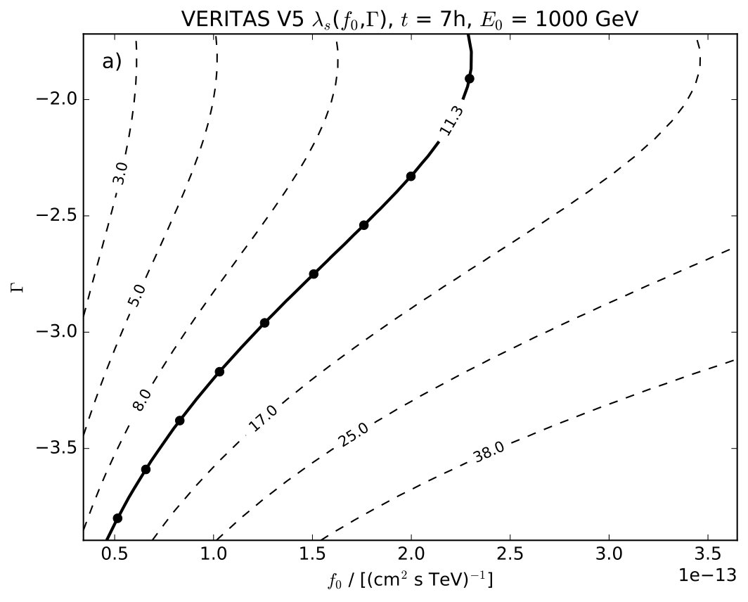 Figure 1
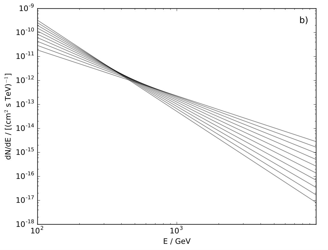 Figure 1
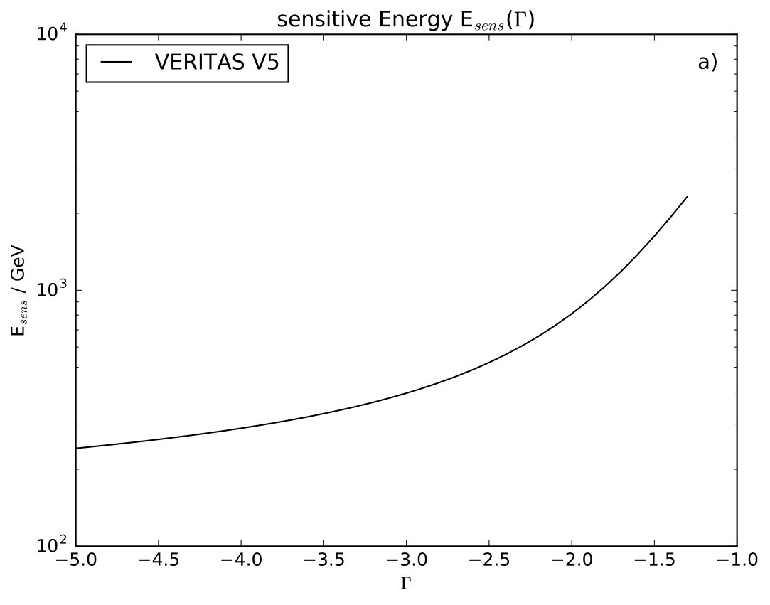 Figure 2
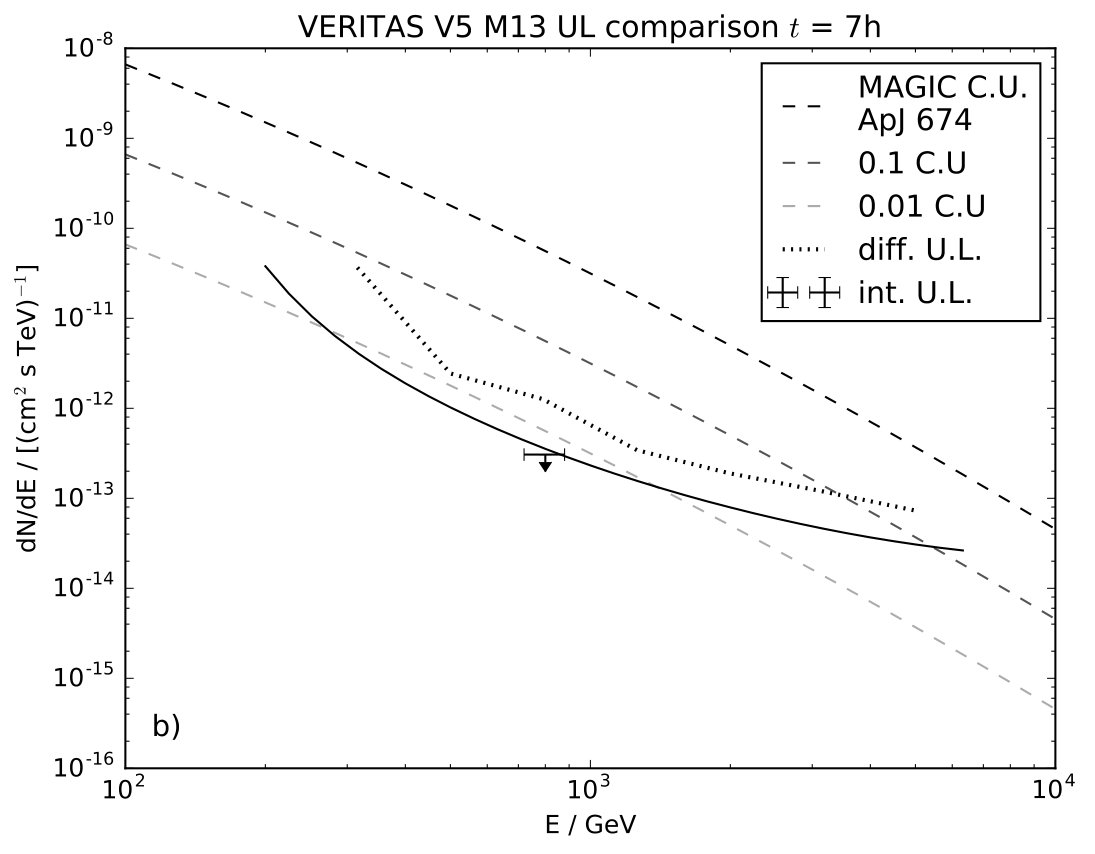 Figure 2
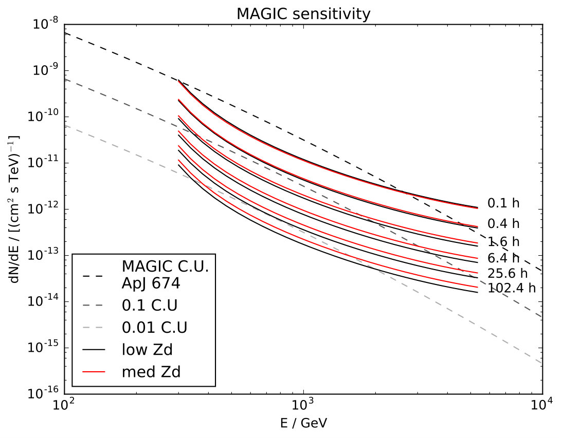 Figure 3
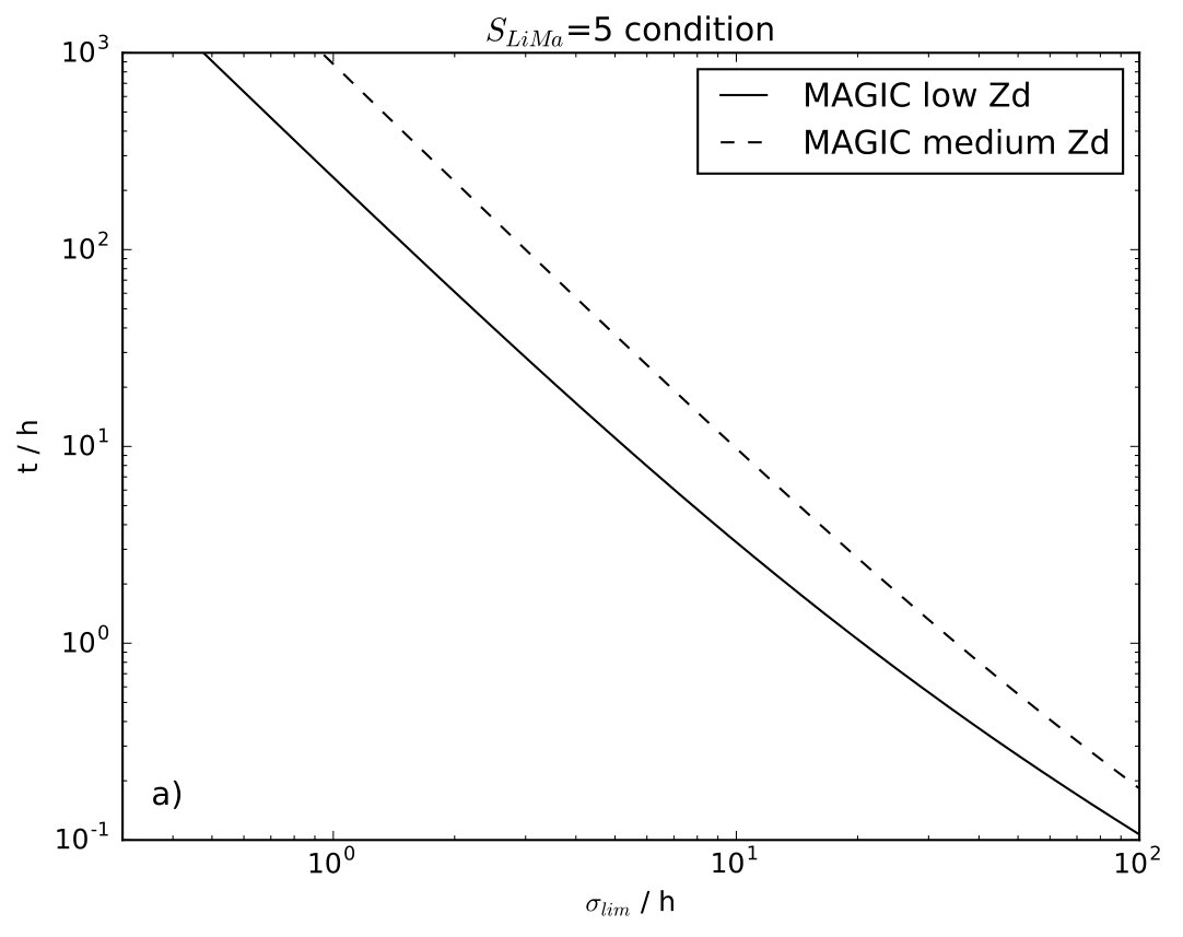 Figure 4
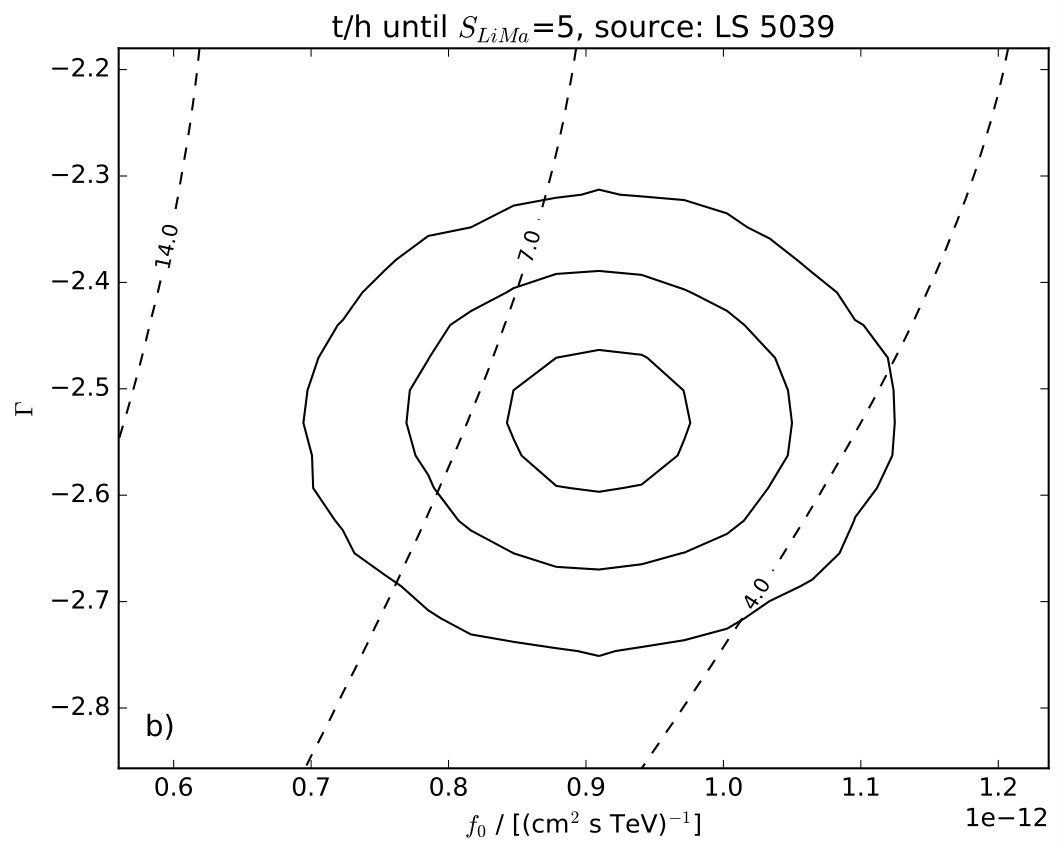 Figure 4
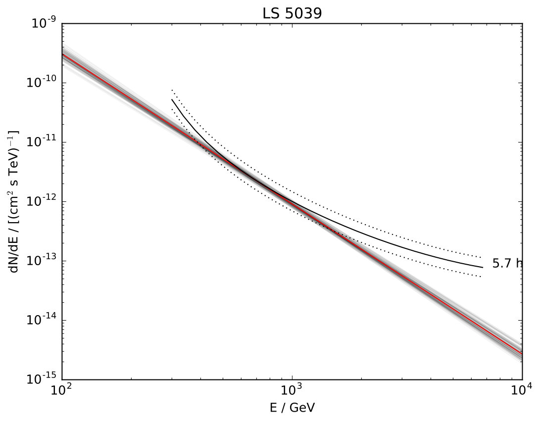 Figure 5
| C.I. | ||||||
|---|---|---|---|---|---|---|
| (h) | ||||||
| 1) | 7 | 0.95 | 1/10 | 55 | 670 | 11.3 |
| mode | extra cut | |||
|---|---|---|---|---|
| (1/h) | ||||
| low Zd | 1) | 1/5 | 7.37 | |
| med. Zd | 1) | 1/5 | 28.83 |
| name | assoc. tevcat | RA | dec | Zd range | ref. | |||
|---|---|---|---|---|---|---|---|---|
| (∘) | (∘) | (h) | ||||||
| Crab | TeV J0534+220 | 83.629 | 22.022 | low | 1) | |||
| HESS J1837-069 | TeV J1837-069 | 279.410 | -6.950 | medium | 2) | ∗ | ||
| W 41 | TeV J1834-087 | 278.690 | -8.780 | medium | 3) | |||
| Cas A | TeV J2323+588 | 350.806 | 58.808 | medium | 4) | |||
| LS 5039 | TeV J1826-148 | 276.563 | -14.842 | medium | 5) | ∗ | ||
| W 49B | TeV J1911+090 | 287.780 | 9.087 | low | 6) | ∗ | ||
| CTB 87 | TeV J2016+372 | 304.008 | 37.220 | low | 7) | ∗ | ||
| 3C 58 | TeV J0209+648 | 31.379 | 64.841 | medium | 8) |
Peer Reviews
No public reviews on file for this paper yet. If you reviewed it on a platform where reviews are public (OpenReview, ICLR, NeurIPS, ICML), you can paste yours below so the community can read it here.
Code & Models
Videos
No videos yet. Explain this paper in a talk, walkthrough, or lecture? Add one.
On integral upper limits assuming power law spectra
and the sensitivity in high-energy astronomy
Max L. Ahnen11affiliation: [email protected]
Institute for Particle Physics, ETH Zurich, 8093 Zurich, Switzerland
Abstract
The high-energy non-thermal universe is dominated by power law-like spectra. Therefore results in high-energy astronomy are often reported as parameters of power law fits, or, in the case of a non-detection, as an upper limit assuming the underlying unseen spectrum behaves as a power law. In this paper I demonstrate a simple and powerful one-to-one relation of the integral upper limit in the two dimensional power law parameter space into the spectrum parameter space and use this method to unravel the so far convoluted question of the sensitivity of astroparticle telescopes.
gamma-rays: general — methods: statistical
1 Introduction
Power law spectra are a general feature in the non-thermal high-energy universe. Often results in high-energy astronomy are reported as parameters of power law fits (e.g. Ackermann et al., 2016; Aharonian et al., 2006b), or, if no source is detected, as a flux limit (e.g. Archambault et al., 2016; Aliu et al., 2012, 2014a; Ahnen et al., 2016b; Aleksić et al., 2015; Abramowski et al., 2014; Aliu et al., 2015; Ahnen et al., 2016a) assuming the unseen spectrum is a power law
[TABLE]
In Eqn. 1 is a freely chosen reference energy, is the flux normalization, and is the spectral index.
The ability of gamma-ray, neutrino, and cosmic-ray telescopes to detect a source depends on their intrinsic parameters and on the external source spectrum (Aleksić et al., 2016; Aharonian et al., 2006d; Murase & Takami, 2008; Bertou et al., 2002; Aartsen et al., 2015). However, even when no significant signal counts are detected, lone would like to put limits on the observed signal flux would allow inference of physical results, as observing nothing is fundamentally different from not observing at all. But what does an upper limit on the signal count rate mean for the spectrum? This question is tightly related to the detection limit of a given instrument. After all, every observer is interested to know: How long does it take to detect my source with an assumed average flux?
Currently, there are only convoluted or partial answers to these two fundamental questions in high-energy astronomy. However, the universal observation of power laws in gamma-ray sources allows framing the questions in the parameter space of the power law.
2 Upper limits in the context of On/Off measurements
In the low count regime of high-energy astronomy one experimental method is well established: The On/Off measurement (Li & Ma, 1983; Rolke et al., 2005; Knoetig, 2014; Abraham et al., 2007; Abbasi et al., 2011). In it, the experimenter would like to measure an imprecisely known background count rate as well as a potential signal count rate. The measurement consists of two observations: The first counts events in a region with potential signal, the second counts events in an adjacent region which is assumed to be signal free. Both regions are related to one another through the ratio of exposures . If the data show no evidence for a source, an upper limit on the signal counts can be calculated using , , and (Rolke et al., 2005; Knoetig, 2014). This limit can be used to infer constraints on the potential source spectrum.
The most constraining upper limits can be extracted from integral upper limits, calculated using the average signal counts integrated over all energies. Then, in order to to make inferences about the source spectrum one, usually, further assumes a certain power law with a common spectral index (Abramowski et al., 2014; Aleksić et al., 2015; Ahnen et al., 2016b; Aliu et al., 2015, 2014a).
[TABLE]
Assuming a steady source, the integrated average signal counts depend on the instrument effective area for each energy , the observation time , and the assumed source spectrum parameter . The limit flux normalization is then calculated such that the resulting power law spectrum would yield the limit
[TABLE]
The result is often reported as integrated source flux above a certain threshold energy
[TABLE]
Implicit in this method is the choice of the power law index which can be extrapolated (Ahnen et al., 2016b), physically motivated (Aliu et al., 2015, 2014a), or hedged to have little impact on the result (Abramowski et al., 2014; Aleksić et al., 2015). However, extrapolating is not always possible and the power law index often varies strongly from source to source (Ackermann et al., 2016), which propagates to a potentially large systematic error in the flux limits.
A method to reduce the systematic error of the choice of power law index and to infer spectral information in the absence of signal is to calculate differential upper limits. Although they are called differential, no observation can measure differentials directly. Therefore, differential upper limits are approximated by upper limits integrated in small bins, assuming a certain power law index and using Eqn. 3 and Eqn. 4. The limit curve obtained in this way still depends on the choice of (Ahnen et al., 2016b), admittedly less than the full integral upper limit. The main issue with differential upper limits is their lower sensitivity due to the binning, which falls short of the real detection capabilities of the instrument.
A more sensitive approach to the influence of the power law index is the decorrelation energy method (Aliu et al., 2012; Archambault et al., 2016). Here, integral upper limits are first calculated assuming three different power law indices. This results in three different limit power laws. The decorrelation energy is then defined as the energy at which their flux and therefore their upper limit estimate depends the least on the power law index. In a final step the weakest of the three upper limits at the decorrelation energy (which turns out to be the upper limit of the central power law index) is reported. While this method better accounts for variations in , it is still not universal as three common power law indices have to be chosen, none of which are distinguished.
In this paper, I demonstrate a more useful approach to integral upper limits than the previously discussed methods. The key insight comes from investigating integral upper limits in the two dimensional parameter space of the power law.
3 Generalized integral upper limits assuming power law spectra
In the following I derive the novel integral upper limit method, and compare it to, a data set from the VERITAS Cherenkov telescope (McCutcheon, 2012). In it, upper limits from an observation of the globular cluster M13 are reported. M13 is measured to host millisecond pulsars (Hessels et al., 2007) and is a popular, yet undetected, target for Cherenkov telescopes (McCutcheon, 2012; Anderhub et al., 2009). In this case the observations took place during the VERITAS epoch V5 (Park, 2016) in 2010. The following components must be specified to calculate any integral upper limit for a specific On/Off measurement:
: Effective area as a function of true energy after all cuts 2. 2.
: Effective observation time 3. 3.
: Choice of criterion on the signal counts limit e.g., Rolke et al. (2005); Knoetig (2014); calculation relies on
- (a)
Choice of credible interval or confidence interval e.g., 2. (b)
: On/Off region exposure ratio 3. (c)
: Number of events in the On region 4. (d)
: Number of events in the Off region
The components used in this section are shown in Tab. 3. The resulting signal limit is calculated using the 95% credible limit on the signal posterior using the method from Knoetig (2014).
When investigating spectra of sources it is important to take the difference between estimated energy and true (or simulated true) energy into account. This relationship is the migration matrix. This means that the effective area measured over estimated energy is a convolution of the effective area over true energy , the migration matrix, and the source spectrum. However, as the method proposed here is an integral limit method, it needs the effective area as a function of the true (simulated) energy . In my case however, I use the commonly reported (McCutcheon, 2012; Aleksić et al., 2016) as an approximation to as no suitable effective areas are published together with the necessary data components.
When examining the family of excluded power laws in the parameter space for the VERITAS M13 observation, the result is Fig 1a). It shows the average signal counts as a function of the power law parameters (Eqn. 3), together with the implicitly defined curve where the average signal counts are equal to the signal limit (Eqn. 4). The power laws on this curve represent the border of the excluded parameter space — the region with higher fluxes to the right is excluded. This plot can already be used to compare models with limits, as sources populate the power law parameter space (Ackermann et al., 2016). However, most physicists compare source spectra and models in the spectrum parameter space.
The following translation of the implicitly defined power law exclusion curve (Fig. 1a) into the spectrum parameter space (Fig. 1b) is key. When looking at a set of power laws from the family of curves on the exclusion line, it becomes apparent that they produce an envelope curve when regarding flux upper limits in the spectrum parameter space. This means that for every assumed power law index there is an energy I call sensitive energy in the spectrum parameter space. At the sensitive energy the limit power law with has, locally, the maximum flux (Eqn. 1), compared to the other power laws on the power law exclusion curve. Therefore, one specific integral flux upper limit is distinguished at , which can be used to construct a one-to-one relation from points on the power law exclusion curve to points in the spectrum parameter space by
[TABLE]
The curve in the spectrum parameter space represents the border of the region, which I call integral spectral exclusion zone.
The necessary conditions for the existence of the integral spectral exclusion zone can be deduced from the method of Lagrange multipliers, which is done in Appendix A. A fundamental analytical result of this is
[TABLE]
where is defined as the average of the natural logarithm of the true energy over sensitive area weighted by the power law
[TABLE]
The example VERITAS is shown in Fig. 2a). To calculate the integral spectral exclusion zone , one has to determine the power law that is locally tangent to the border of the zone at energy . This can be done in two ways:
Use the Lagrange multiplier results.
- (a)
Calculate numerically by inverting (using Eqn. 7). 2. (b)
Calculate by solving the power law exclusion line constraint Eqn. 4
[TABLE]
where is defined as the spectrum-weighted acceptance
[TABLE] 3. (c)
Insert parameters in
[TABLE] 2. 2.
Calculate Eqn. 6 by maximizing the local flux under constraints directly.
What is the physical meaning of and the integral spectral exclusion zone? In case a power law with index crosses into the integral spectral exclusion zone, its corresponding implicitly defined (Eqn. 4) upper limit flux normalization at the sensitive energy is lower. Therefore, the border of the integral spectral exclusion zone is the physical boundary where every source with a power law spectrum crossing it would be detected, independent of . From this point of view, is the energy at which a source with a given power law index is best constrained. As the sensitive energy is a monotonically increasing function of (see Appendix A), this yields the intuitive result that harder spectra are better constrained at higher energies and that softer spectra are better constrained at lower energies.
Applying this method to the VERITAS M13 data set results in Fig 2b). Here, the integral spectral exclusion zone is calculated maximizing the logarithm of the flux under constraints directly (see Eqn. 6) using the scipy.optimize Python library (Jones et al., 2001–). The integral spectral exclusion zone is compatible with the reported integral limit at the decorrelation energy and is about 5 times more sensitive than the reported differential limit. The VERITAS method of reporting an integral upper limit at the decorrelation energy (see Sec. 2) approximates the integral spectral exclusion zone at one point, which is also apparent from the method. In this sense the integral spectral exclusion zone is a generalization of the decorrelation energy method.
4 Application: The sensitivity of astroparticle telescopes
One important application of the integral spectral exclusion zone is the fundamental question: What sources can a certain instrument detect? After all, upper limits are a statement of sensitivity. Therefore, the current methods tackling this question are equivalent to the current methods of calculating upper limits described in Sec. 2.
First, there are integral methods assuming a certain power law index . Among the possible power laws, the power law with minimum flux normalization which is required for a detection in a certain observation time is chosen. This is often reported as a function of observation time (Aharonian et al., 2006d). A similar approach is to report the integral sensitivity as a function of the minimum flux required for detection above a given threshold energy (Aleksić et al., 2016). However, this method does not constitute a full analysis as the last cut (in energy) is unspecified. Therefore, it can not be compared to other sensitivities easily. Furthermore, the power law index problem persists: What if the source has a different ?
Second, authors report sensitivities as differential upper limits (Aleksić et al., 2016; Bernlöhr et al., 2013), solving the power law index issue. This method is also used to compare instrument sensitivities (Funk et al., 2013) but, as discussed in Sec 2, being a differential limit, it falls short of the real detection capabilities of the instruments.
I demonstrate my novel method using the latest published performance data from the MAGIC Cherenkov telescope (Aleksić et al., 2016). For a given On/Off measurement analysis, the following components define the sensitivity of an astroparticle telescope to detect sources with power law spectra:
: Effective area as a function of true energy after all cuts 2. 2.
: The sensitivity consensus criterion is, unlike the upper limit criterion, five standard deviations calculated according to Li & Ma (1983). Subsequently required are
- (a)
: On/Off normalization factor 2. (b)
: Background event rate in the On region, estimated from simulations or independent Off region data
Unfortunately, it is not common for Cherenkov telescope collaborations to publish , , and coherently for selected and specific analyses. This means that it is not possible, outside of a telescope collaboration, to calculate the time until an analysis detects a power law source without further assumptions. I therefore make the following assumptions (see Tab 4) in order to use the published MAGIC results (Aleksić et al., 2016):
: Possible values for stated in that publication are and . Given that similar Cherenkov telescopes use even more Off regions (see Tab. 3), I assume the more sensitive value is reasonable. 2. 2.
: The reported effective area is not given after all cuts. The authors used an additional energy cut at to achieve the most sensitive instrument. Therefore, to approximate , I use the reported with a threshold at convoluted with the energy resolution stated in Aleksić et al. (2016).
Table 4 further contains the MAGIC analyses specific zenith distance domain names (low and medium ) and background rates .
The integral spectral exclusion zone method can now be applied to the MAGIC sensitivity question. When investigating the sensitivity, most authors (Aleksić et al., 2016; Aharonian et al., 2006d; Park, 2016) use five standard deviations calculated according to Equation 17 in Li & Ma (1983) as sensitivity limit criterion. The connection between this criterion and the signal counts limit can be constructed from assuming a constant background flux in an area with On region exposure
[TABLE]
where the signal rate limit (to be inferred) is related to the signal counts limit via the observation time
[TABLE]
When inserting Eqn 12 and Eqn 13 into the limit condition , one can numerically solve for . Then, Eqn. 14 can be used to calculate . The Li&Ma criterion is only valid for count numbers which are “not too few” (Li & Ma, 1983). Therefore, it is common (Aleksić et al., 2016; Park, 2016; Aharonian et al., 2006d) to use an additional limit, which is imposing to measure at least ten gamma-ray signal counts in the On region .
In this way, the instrument- and analysis-specific sensitivities can be calculated for any observation time using the integral spectral exclusion zone method.
The result, applied to the MAGIC telescope analyses from Tab. 4, is shown in Fig. 3. It agrees well with MAGIC’s ability (Aleksić et al., 2016) to detect a Crab nebula-like source with 1% Crab nebula flux within .
In the case of specific sources, it is useful to return to the power law parameter space . Table 4 shows eight selected galactic TeV emitting gamma-ray sources, observable from the MAGIC site (Latitude ) at low or medium zenith distances. This implies source declinations . As the MAGIC background rate parameters from Tab. 4 are valid for point-like sources, only MAGIC quasi point-like sources (up to a mean extension of ) are considered. In the following, I use the LS 5039 low state flux as an example for how to estimate the necessary observation time until detection.
The average time to detect a certain power law in the power law parameter space must be calculated by numerically inverting the signal rate limit . Figure 4a) shows as a function of the signal rate for the low Zd and medium Zd MAGIC analyses.
Then, the power law limit curve Eqn 4 can be reformulated using the average signal counts function (Eqn. 3), the power law spectrum (Eqn. 1), and as
[TABLE]
Finally, the average estimated observation time until detection (Eqn. 15) can be calculated as a function of the power law parameters . This is demonstrated in Fig. 4b) together with the measured LS 5039 parameter confidence intervals (Aharonian et al., 2006a) assuming uncorrelated normal distributed errors in and . The data indicates that MAGIC, using the analysis parameters from Tab. 4, would need in order to detect this source.
To quantify , one can sample from the parameter space according to the LS 5039 parameter errors and calculate the histogram of times to detection. I report the times to detection as the median time with asymmetric errors calculated from the 16th percentile and the 84th percentile in Tab 4. In the case of LS 5039, this results in an estimated MAGIC time to detection of . Four out of eight calculated are predictions as MAGIC has not reported detections on HESS J1837-069, LS 5039, W 49B, and CTB 87.
Finally, one can illustrate the estimated time to detection using the integral spectral exclusion zone, which is done in Fig. 5. It shows the simple but powerful interpretation of the integral spectral exclusion zone as the instrument detection capability — the border of the region in the spectrum parameter space which any detectable power law would cross.
5 Discussion
The calculations in this manuscript are done using the true energy , as I only consider integral results (see Sec. 3). Therefore, limited energy resolution and migration do not affect the integral spectral exclusion zone, as a power law source does indeed emit with its true individual spectrum and an instrument measures the events according to . This is the case even when one is unable to reconstruct the individual event energies at all. Therefore, it is possible to know the sensitivity of an instrument to detect power law sources without reconstructing the energy of individual events.
There are several cases when sources reveal additional curvature, besides the general power law behavior, after measuring them with high significance and low statistical uncertainty. However, the upper limit question and the sensitivity question for an individual telescope analysis only consider what happens at the detection threshold and only what happens in the limited energy domain of (see Eqn. 3). There, basically every source in astroparticle physics appears as power law initially. Therefore, I argue that the integral spectral exclusion zone is applicable, even when source spectra deviate “not too much” from power laws.
In this manuscript I only considered On/Off measurements so far, which infer results in view of Poissonian signal-and-noise experiments (see Sec. 2), but there may be other cases when, for instance, no background is expected and can be calculated from a single Poisson process producing . In general, there are plenty of statistical approaches to choose from. However, the details of calculating are up to each individual experimentalist and what method she believes in. The signal count limit , formulated as constraint in Eqn 6, is only the interface of my integral spectral exclusion zone method with the world of statistics: It stays the same while the statistical methods may be exchanged.
6 Conclusion
Many high-energy astronomers struggle with the implications of non-detections and instrument limits. The universal observation of power laws in high-energy sources allows framing these problems in the parameter space of the power law model. A simple and powerful one-to-one relation of the integral spectral limit in the power law parameter space into spectra makes it possible to construct the integral spectral exclusion zone. This integral spectral exclusion zone demonstrates what astroparticle telescopes are actually capable of detecting – and how long it will take. In this way one can easily compare instrument performances, optimize analysis algorithms, and test model predictions of high-energy astrophysics.
A python package implementing the methods from this manuscript can be found at https://github.com/mahnen/gamma_limits_sensitivity
I would like to thank Adrian Biland, Sebastian A. Mueller, Scott Lindner, Camila Shirota and Dariusz Gora for support, discussions, and valuable comments on the article.
Appendix A Application of the Lagrange multiplier method for calculating
the integral spectral exclusion zone
Motivated by the results shown in Fig. 1, I assume the existence of a maximum flux (Eqn. 1) given the external constraint (Eqn. 4). Then, the necessary conditions for the existence of the integral spectral exclusion zone can be deduced from the method of Lagrange multipliers. The first step is the construction of the problem specific Lagrange function by joining the function to be maximized to the external constraint using a Lagrange multiplier
[TABLE]
where is an abbreviation for the spectrum weighted acceptance
[TABLE]
By taking the gradient with respect to the parameters and equating it to zero one gets a set of equations
[TABLE]
which, together with the external constraint Eqn. 4, constitute the necessary conditions. Equation A4 solved for gives
[TABLE]
This equation inserted back into Eqn. A3 results in
[TABLE]
When interchanging the integral and differentiation in the explicit formula of and solving Eqn A6 for the energy E the result is
[TABLE]
where is an abbreviation for the average of the natural logarithm of the energy over the spectrum weighted acceptance
[TABLE]
is independent of , which is a reasonable result for a scale factor. I identify the energy at which the Lagrange function has a maximum with the sensitive Energy in Sec 3.
Equation A8 shows that the existence of the integral spectral exclusion zone is a direct consequence of the physical argument that there can not be infinite counts which leads to the normalizability of the spectrum weighted acceptance (finite numerator and denominator in Eqn. A8). The average natural logarithm of the energy is an increasing function of , as harder spectra produce higher energy events more frequently. Therefore, is also an increasing function, which means it is invertible. Finally, one can take Eqn. A7, solve it numerically for , and find the last remaining undetermined parameter by solving the so far unused constraint function Eqn. 4, which is shown in Eqn. 9.
The reference list from the paper itself. Each links out to its DOI / PubMed record.
- 1Aartsen et al. (2015) Aartsen, M. G., Abraham, K., Ackermann, M., Adams, J., et al. 2015, Ap J, 809, 98
- 2Abbasi et al. (2011) Abbasi, R., Abdou, Y., Abu-Zayyad, T., et al. 2011, Phys. Rev. D, 84, 022004
- 3Abdalla et al. (2016) Abdalla, H., Abramowski, A., Aharonian, F., et al. 2016, ar Xiv preprint ar Xiv:1609.00600
- 4Abraham et al. (2007) Abraham, J., Aglietta, M., Aguirre, C., et al. 2007, Astropart. Phys., 27, 244
- 5Abramowski et al. (2014) Abramowski, A., Aharonian, F., Benkhali, F. A., et al. 2014, A&A, 564, A 9
- 6Ackermann et al. (2016) Ackermann, M., Ajello, M., Atwood, W. B., et al. 2016, Ap JS, 222, 5
- 7Aharonian et al. (2004) Aharonian, F., Akhperjanian, A. G., Beilicke, M., et al. 2004, Ap J, 614, 897
- 8Aharonian et al. (2006 a) Aharonian, F., Akhperjanian, A. G., Bazer-Bachi, A. R., et al. 2006 a, A&A, 460, 743
