Fast initial conditions for Glauber dynamics
Eyal Lubetzky, Allan Sly

TL;DR
This paper introduces new methods using information percolation to analyze the mixing times of Glauber dynamics for the 1D Ising model from various initial states, revealing temperature-dependent optimal starting conditions.
Contribution
It provides the first analysis of mixing times from non-worst-case initial states in Glauber dynamics, showing the alternating initial condition is fastest at high temperatures.
Findings
Alternating initial condition is fastest at high temperatures.
Mixing time at the optimal initial condition is faster than at infinite temperature.
The dominant test function varies with temperature, switching from autocorrelation to Hamiltonian.
Abstract
In the study of Markov chain mixing times, analysis has centered on the performance from a worst-case starting state. Here, in the context of Glauber dynamics for the one-dimensional Ising model, we show how new ideas from information percolation can be used to establish mixing times from other starting states. At high temperatures we show that the alternating initial condition is asymptotically the fastest one, and, surprisingly, its mixing time is faster than at infinite temperature, accelerating as the inverse-temperature ranges from 0 to . Moreover, the dominant test function depends on the temperature: at it is autocorrelation, whereas at it is the Hamiltonian.
Click any figure to enlarge with its caption.
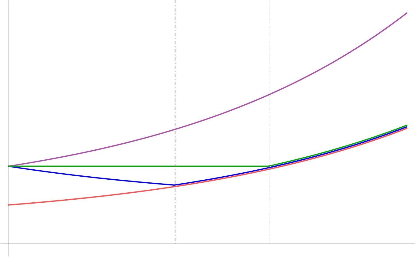 Figure 1
Peer Reviews
No public reviews on file for this paper yet. If you reviewed it on a platform where reviews are public (OpenReview, ICLR, NeurIPS, ICML), you can paste yours below so the community can read it here.
Videos
No videos yet. Explain this paper in a talk, walkthrough, or lecture? Add one.
Fast Initial Conditions for Glauber Dynamics
Eyal Lubetzky
Eyal Lubetzky Courant Institute of Mathematical Sciences
New York University
New York, NY 10012, USA.
and
Allan Sly
Allan Sly Department of Mathematics
Princeton University
Princeton, NJ 08544, USA, and Department of Statistics
UC Berkeley
Berkeley, CA 94720, USA.
Abstract.
In the study of Markov chain mixing times, analysis has centered on the performance from a worst-case starting state. Here, in the context of Glauber dynamics for the one-dimensional Ising model, we show how new ideas from information percolation can be used to establish mixing times from other starting states. At high temperatures we show that the alternating initial condition is asymptotically the fastest one, and, surprisingly, its mixing time is faster than at infinite temperature, accelerating as the inverse-temperature ranges from 0 to . Moreover, the dominant test function depends on the temperature: at it is autocorrelation, whereas at it is the Hamiltonian.
1. Introduction
In the study of mixing time of Markov chains, most of the focus has been on determining the asymptotics of the worst-case mixing time, while relatively little is known about the relative effect of different initial conditions. The latter is quite natural from an algorithmic perspective on sampling, since one would ideally initiate the dynamics from the fastest initial condition. However, until recently, the tools available for analyzing Markov chains on complex systems, such as the Ising model, were insufficient for the purpose of comparing the effect of different starting states; indeed, already pinpointing the asymptotics of the worst-case state for Glauber dynamics for the Ising model can be highly nontrivial.
In this paper we compare different initial conditions for the Ising model on the cycle. In earlier work [LS4], we analyzed three different initial conditions. The all-plus state is provably the worst initial condition up to an additive constant. Another is a quenched random condition chosen from , the uniform distribution on configurations, which with high probability has a mixing time which is asymptotically as slow. A third initial condition is an annealed random condition chosen from , i.e., to start at time 0 from the uniform distribution, which is asymptotically twice as fast as all-plus.
Here we consider two natural deterministic initial configurations. The first is the alternating sequence
[TABLE]
which we will show is asymptotically the fastest deterministic initial condition—yet strictly slower than starting from the annealed random condition—for all (at they match). The second is the bi-alternating sequence
[TABLE]
For convenience we will assume that is a multiple of 4, which ensures that the configurations are semi-translation invariant and turns both sequences into eigenvectors of the transition matrix of simple random walk on the cycle. (This is not necessary for the main result but leads to cleaner analysis.)
In what follows, set , and let denote the time it takes the dynamics to reach total variation distance at most from stationarity, starting from the initial condition .
Theorem 1**.**
For every and there exist and such that the following hold for Glauber dynamics for the Ising model on the cycle at inverse-temperature for all .
- (i)
Alternating initial condition:
[TABLE] 2. (ii)
Bi-alternating initial condition:
[TABLE]
Surprisingly, the mixing time for the alternating initial condition begins as actually faster than the infinite temperature model: it decreases as a function of before increasing when .
The following theorem summarizes the bounds we proved in [LS1, LS4] for the all-plus and random initial conditions. See Figure 1 for the relative performance of all these different initial conditions.
Theorem 2** ([LS1, LS4]).**
In the same setting of Theorem 1, the following hold.
- (i)
All-plus initial condition :
[TABLE] 2. (ii)
Quenched random initial condition:
[TABLE] 3. (iii)
Annealed random initial condition:
[TABLE]
(Note that, in the case of the all-plus initial conditions, the mixing time is known in higher precision: it was shown [LS1, LS4] to be within an additive constant (depending on and ) of .)
The upper bounds on the mixing times in Theorem 1 rely on the information percolation framework introduced by the authors in [LS4]. The asymptotically matching lower bounds in that theorem are derived from two test functions: the autocorrelation function, which for instance matches our upper bound on the alternating initial condition for ; and the Hamiltonian test function, which gives rise to the following lower bound on every deterministic initial condition.
Proposition 3**.**
Let be Glauber dynamics for the Ising model on at inverse-temperature . For every sequence of deterministic initial conditions , the dynamics at time
[TABLE]
is at total variation distance from equilibrium; that is,
[TABLE]
As a consequence of this result and Theorem 1, Part (i), we see that the initial condition is indeed the optimal deterministic one in the range , and that marks the smallest where a deterministic initial condition can first match the performance of the annealed random condition.
The mixing time estimates in Theorem 1 (as well as those in Theorem 2) imply, in particular, that Glauber dynamics for the Ising model on the cycle, from the respective starting configurations, exhibits the cutoff phenomenon—a sharp transition in its distance from stationarity, which drops along a negligible time period known as the cutoff window (here, , vs. which is of order ) from near its maximum to near 0. Until recently, only relatively few occurrences of this phenomenon, that was discovered by Aldous and Diaconis in the early 1980’s (see [Aldous, AD, DiSh, Diaconis]), were rigorously verified, even though it is believed to be widespread (e.g., Peres conjectured [LLP]Conjecture 1,[LPW]§23.2 cutoff for the Ising model on any sequence of transitive graphs when the mixing time is of order ); see [LPW]*§18.
For the Ising model on the cycle, the longstanding lower and upper bounds on from a worst-case initial condition differed by a factor of 2—in our notation, and —while cutoff was conjectured to occur (see, e.g., [LPW]*Theorem 15.4, as well as [LPW]*pp. 214,248 and Question 8 in p. 300). This was confirmed in [LS1], where the above lower bound was shown to be tight, via a proof that relied on log-Sobolev inequalities and applied to , for any dimension , so long as the system features a certain decay-of-correlation property known as strong spatial mixing. This result was reproduced in [LS4] (with a finer estimate for the cutoff window) via the new information percolation method. Soon after, a remarkably short proof of cutoff for the cycle—crucially hinging on the correspondence between the one-dimensional Ising model and the “noisy voter” model—was obtained by Cox, Peres and Steif [CPS]. It is worthwhile noting that the arguments both in [CPS] and in [LS1] are tailored to worst-case analysis, and do not seem to be able to treat specific initial conditions as examined here. In contrast, the information percolation approach does allow one to control the subtle effect of various initial conditions on mixing.
To conclude this section, we conjecture that Proposition 3 also holds for , i.e., that is asymptotically fastest among all the deterministic initial conditions at all . We further conjecture that the obvious generalization of to for (a checkerboard for ) is the analogous fastest deterministic initial condition throughout the high-temperature regime.
2. Update support and information percolation
In this section we define the update support and use the framework of information percolation (see the papers [LS3, LS5] as well as the survey paper [LS6] for an exposition of this method) to upper bound the total variation distance with alternating and bi-alternating initial conditions.
2.1. Basic Notation
The Ising model on a finite graph with vertex-set and edge-set is a distribution over the set of configurations ; each is an assignment of plus/minus spins to the sites in , and the probability of is given by the Gibbs distribution
[TABLE]
where is a normalizer (the partition-function) and is the inverse-temperature, here taken to be non-negative (ferromagnetic). The (continuous-time) heat-bath Glauber dynamics for the Ising model is the Markov chain—reversible w.r.t. the Ising measure —where each site is associated with a rate-1 Poisson clock, and as the clock at some site rings, the spin of is replaced by a sample from the marginal of given all other spins. See [Martinelli97] for an extensive account of this dynamics. In this paper we focus on the graph and will let denote the Glauber dynamics Markov chain on .
An important notion of measuring the convergence of a Markov chain to its stationarity measure is its total-variation mixing time, denoted for a precision parameter . From initial condition we denote
[TABLE]
and the overall mixing time as measured from a worst-case initial condition is
[TABLE]
where here and in what follows denotes the probability given , and the total-variation distance is defined as .
2.2. Information percolation clusters
The dynamics can be viewed as a deterministic function of and a random “update sequence” of the form , where are the update times (the ringing of the Poisson clocks), the ’s are i.i.d. uniformly chosen sites (which clocks ring), and the ’s are i.i.d. uniform variables on (to generate coin tosses). There are a variety of ways to encode such updates but in the case of the one-dimensional model there is a particularly useful one. We add an extra variable which is a randomly selected neighbor of Then given the sequence of the updates are processed sequentially as follows: set ; the configuration for all () is obtained by updating the site via the unit variable as follows: if update the spin at to a uniformly random value and with probability set it to the spin of .
With this description of the dynamics, we can work backwards to describe how the configurations at time (or at any intermediate time) depend on the initial condition. The update support function, denoted , as introduced in [LS1], is the random set whose value is the minimal subset which determines the spins of given the update sequence along the interval .
We now describe the support of a vertex as it evolves backwards in time from to . Initially, ; then, updates in reverse chronological order alter the support: given the next update , if and then is set to , and if then it is set to . Thus, backwards in time performs a continuous-time simple random walk with jump rate which is killed at rate . We refer to the full trajectory of the update support of a vertex as the history of the vertex. The survival time for a walk is exponential and so for ,
[TABLE]
For general sets we have that and taken together the collection of the update supports of the vertices are a set of coalescing killed continuous-time random walks.
A key use of these histories is to effectively bound the spread of information, as achieved by the following lemma.
Lemma 2.1**.**
For any we have that
[TABLE]
Proof.
By equation (2.2) we have that so it is sufficient to show that
[TABLE]
This probability is bounded above by the probability of a rate continuous-time random walk to make at least jumps by time . This is exactly the probability that a Poisson with mean is at least , which satisfies the required bound by standard tail bounds. ∎
3. Upper bounds
We will consider the dynamics run up to time and derive an upper bound on its mixing time. We will first estimate the total variation distance not of the full dynamics but simply at a single vertex from initial conditions and .
Lemma 3.1**.**
For we have that,
[TABLE]
Proof.
We will begin with the case of initial condition . Of course is the uniform measure on . The history is killed before time [math] with probability and on this event is uniform on . Condition that it survives to time [math] and let . This is simply a continuous-time random walk on which switches state at rate . Thus,
[TABLE]
It therefore follows that , and altogether,
[TABLE]
The case of follows similarly, with the exception that has jump rate since it only switches sign with probability each step. ∎
3.1. Update Support
In this subsection we analyse the geometry of the update support similarly to [LS1] in order to approximate the Markov chain as a product measure. Let and define the support time as . By Lemma 2.1 we expect the histories to not travel “too far” along the time-interval to ; precisely, if we define as the event
[TABLE]
then by Lemma 2.1,
[TABLE]
The following event says that the support at time clusters into small well separated components. Let be the event that there exists a set of intervals that (i) cover the support:
[TABLE]
(ii) have logarithmic size:
[TABLE]
and (iii) are well-separated:
[TABLE]
Lemma 3.2**.**
We have that .
Proof.
Define the following intervals on :
[TABLE]
Restricting to , we let
[TABLE]
Since we have that by Lemma 3.1. Next, let be the event
[TABLE]
By a union bound and equation (2.2), we have that
[TABLE]
and so
[TABLE]
Moreover, conditional on the events are conditionally independent since the history of is determined by the updates within the set which are disjoint. Hence, for all ,
[TABLE]
hence,
[TABLE]
Taking a union bound over all we have that
[TABLE]
We have thus arrived at the following: with probability at least , for every there exists a block of consecutive vertices whose histories are killed before within distance on both the right and the left, implying the existence of the decomposition and completing the lemma. ∎
When the event holds we will assume that there is some canonical choice of the ’s. We set
[TABLE]
On the event that both and hold, the sets are disjoint, and satisfy
[TABLE]
We will make use of Lemma 3.3 from [LS3], a special case of which is the following.
Lemma 3.3** ([LS3]).**
For any and any set of vertices we have that
[TABLE]
Using this result, we have that
[TABLE]
3.2. Coupling with product measures
On the event we couple and with product measures. Since the ’s depend only on the updates along the interval and are independent of the dynamics up to time we will treat the as fixed deterministic sets satisfying (3.6). Let be a product measure of copies of . Then, by the exponential decay of correlation of the one-dimensional Ising model,
[TABLE]
Next, let be independent copies of the dynamics up to time . Define the event
[TABLE]
and for each define the analogous event
[TABLE]
where is the support function for the dynamics . From Lemma 2.1, together with a union bound, we infer that
[TABLE]
Let denote conditioned on and, similarly, let denote conditioned on . Then
[TABLE]
and so
[TABLE]
Now, since the laws of the for distinct depend on disjoint sets of updates, they are independent and equal in distribution to , hence
[TABLE]
Since is conditioned on ,
[TABLE]
Combining the previous three equations we find that
[TABLE]
Thus, to show that \big{\|}\mathbb{P}_{x_{0}}\left(X_{t_{\star}}\in\cdot\right)-\pi\big{\|}_{\textsc{tv}}\to 0 it is sufficient to prove that
[TABLE]
3.3. Local distance
Let , and for each set
[TABLE]
with if .
First we bound the right tail of the distribution of . If then at least histories from have survived to time and not intersected. Hence, by equation (2.2),
[TABLE]
Therefore, for we see that
[TABLE]
Let denote the event that for all we have that . By (3.11),
[TABLE]
and so implies that . On the event , we define
[TABLE]
Applying Lemma 3.3 we have that
[TABLE]
Lemma 3.4**.**
There exists such that, for every and ,
[TABLE]
Proof.
We will consider the case of , the proof for follows similarly. Let denote the first time the history coalesces to a single point:
[TABLE]
with the convention if . By equation (2.2),
[TABLE]
Denote the vertex . By Lemmas 3.1 and 3.3 we have that
[TABLE]
We estimate the right hand side as follows:
[TABLE]
where the final inequality follows by taking the maximal term in the sum. This, together with (3.14), completes the proof of the lemma. ∎
We now appeal to the -to- reduction developed in [LS1, LS3]. Recall that the -distance on measures is defined as
[TABLE]
and set
[TABLE]
By [LS3]*Proposition 7,
[TABLE]
We are now ready to prove the upper bound for the main theorem.
Proof of Theorem 1, Upper bound.
Again we focus on the case of . Set
[TABLE]
With this choice of we have that and so, by equations (3.10), (3.3) and (3.17), it is sufficient to show that
[TABLE]
Since each vertex is either plus or minus with probability that is uniformly bounded below by , given any choice of conditioning on the other vertices, we have that
[TABLE]
Comparing the and bounds we have that for any measures and set ,
[TABLE]
Thus, by Lemma 3.4,
[TABLE]
for some . Finally, by equation (3.11)
[TABLE]
Combining the previous two inequalities implies that and hence we have that
[TABLE]
as required. The proof for follows similarly for the choice of
[TABLE]
4. Lower bounds
In order to establish the lower bound we will analyze two separate test functions. First, in order to analyze our test functions, we establish the following decay of correlation bound.
Lemma 4.1**.**
Let such that and let be functions with . Then for any initial condition and time we have that
[TABLE]
Proof.
We will prove the result by showing that can be approximated locally. Let and so the are disjoint. Let denote the sigma-algebra of generated by updates in and set . Since the are disjoint the depend on independent updates and so are independent. Let
[TABLE]
be the event in Lemma 2.1. On the event , the random variables are completely determined by the initial condition and the updates in and so . Thus,
[TABLE]
and hence
[TABLE]
which completes the proof. ∎
Since the above bound is uniform in by taking to infinity we get the result for given by the stationary measure as well.
4.1. Autocorrelation test functions
The magnetization test function achieves, at least up to an additive constant, the mixing time from the all-plus initial condition, which is asymptotically the worst-case (see [LS4]). In this light it is natural to consider test functions for and based on the autocorrelation, . This can be seen as a special case of a test function based on conditional expectations,
[TABLE]
Because of the special structure of the histories as a killed random walk the expectation has the following useful representation. Let be the semigroup of a continuous-time rate-1 simple random walk on . Then by the killed random walk representation we have that
[TABLE]
The eigenvectors of are with eigenvalues for . Since the simple random walk is reversible with uniform stationary distribution we can write an orthonormal basis of real eigenvectors with eigenvalues . Not that both and are eigenvectors of with eigenvalues and respectively and in fact is the largest eigenvalue. We first give a condition for the chain to not be sufficiently mixed starting from .
Lemma 4.2**.**
If for a sequence of initial conditions and time points we have
[TABLE]
then
[TABLE]
Proof.
Let be distributed according to the stationary distribution. Then by symmetry,
[TABLE]
while
[TABLE]
To estimate the variance, observe that
[TABLE]
By Lemma 4.1, this is at most
[TABLE]
where the final inequality follows by the rearrangement inequality. Since Lemma 4.1 also applies to the stationary distribution, we further have
[TABLE]
Our test function considers the set A=\big{\{}x\in\{\pm 1\}^{\mathbb{Z}/n\mathbb{Z}}:R_{x_{0},t}(x)\geq\frac{1}{2}e^{-2\theta t}\|P_{(1-\theta)t}x_{0}\|_{2}^{2}\big{\}}. Therefore, by Chebyshev’s inequality,
[TABLE]
and so by the assumption of the lemma . Similarly,
[TABLE]
so which completes the lemma. ∎
We can now establish Proposition 3, giving a lower bound for any deterministic initial condition.
Proof of Proposition 3.
Writing we have that
[TABLE]
where the inequality follows from the fact that all the eigenvalues are bounded by 2. Thus,
[TABLE]
and so, by Lemma 4.2, we have that , as claimed. ∎
This gives the right bound in the case of since it is an eigenvector of eigenvalue 2. For we get a stronger lower bound. Since it has eigenvalue 1,
[TABLE]
So, taking ,
[TABLE]
and hence by Lemma 4.2 we have that
[TABLE]
4.2. Hamiltonian test functions
The alternating initial condition is an extreme value for the Hamiltonian and measuring its convergence to stationarity gives another test of convergence. Such test functions were studied in [LS4] to analyze the a random annealed initial condition. To treat and in a unified manner, consider the function given by
[TABLE]
For every and we have that, by Lemma 4.1,
[TABLE]
If is taken from the stationary distribution by taking a limit as , then we also have that . Let denote the set of all histories of the vertices from time , and consider . If the histories of and merge then and must take the same value and . If the histories do not merge and at least one is killed before reaching time 0 then it is equally likely to be so . Thus, the boundary condition can only play a role when both histories survive to time 0 and do not merge, as captured by the event
[TABLE]
Let be an independent configuration distributed as and let denotes the expectation started from the stationary measure. Then
[TABLE]
as the ferromagnetic Ising model is positively correlated. In a graph with two vertices connected by an edge, the correlation of spins of the Ising model can be found to be . Correlations are monotone in the edges of the graph, so for neighboring vertices in we have . It was shown in the proof of Theorem 6.4 of [LS4] that
[TABLE]
and so
[TABLE]
We will compare this bound with the behavior under the initial conditions and .
Claim 4.3**.**
For and we have that
[TABLE]
Proof.
We first treat the case of . Let and be independent rate-() continuous-time simple random walks with initial conditions and . Let denote the first time the walks hit each other and . By the killed random walk representation of the histories, we have that
[TABLE]
Note that is itself a Markov chain with state space and transition rate , and so
[TABLE]
Thus, since by the definition of , and , applying (4.5) we get
[TABLE]
Hence, .
For , the process is again a Markov chain but with transition rate . The requirement that is a multiple of 4 was chosen to ensure that . The argument is otherwise unchanged. ∎
Combining Lemma 4.5 with equation (4.2), we obtain that
[TABLE]
and thus
[TABLE]
We are now ready to prove the second lower bound.
Lemma 4.4**.**
Set
[TABLE]
For we have
[TABLE]
Proof.
Denote by the event
[TABLE]
By Chebyshev’s inequality and equations (4.2) and (4.6)
[TABLE]
and similarly
[TABLE]
Hence, , as claimed. ∎
Proof of Theorem 1, Lower bound.
The case of follows from combining Proposition 3 and Lemma 4.4, while the lower bound for follows from equation (4.1) and Lemma 4.4. ∎
Acknowledgements
We thank Yuval Peres for helpful discussions.
References