Improved stability for analytic quasi-convex nearly integrable systems and optimal speed of Arnold diffusion
Jianlu Zhang, Ke Zhang

TL;DR
This paper enhances the understanding of stability in analytic quasi-convex nearly integrable Hamiltonian systems, achieving optimal stability results that align with the maximum possible speed of Arnold diffusion.
Contribution
It provides an improved, optimal Nekhoroshev stability estimate for these systems, matching the fastest known Arnold diffusion speed.
Findings
Achieved optimal Nekhoroshev stability bounds.
Matched the stability results with the maximum speed of Arnold diffusion.
Enhanced theoretical understanding of Hamiltonian system stability.
Abstract
We improve the global Nekhoroshev stability for analytic quasi-convex nearly integrable Hamiltonian systems. The new stability result is optimal, as it matches the fastest speed of Arnold diffusion.
Click any figure to enlarge with its caption.
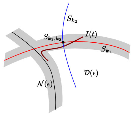 Figure 1
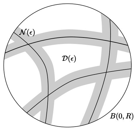 Figure 2
Peer Reviews
No public reviews on file for this paper yet. If you reviewed it on a platform where reviews are public (OpenReview, ICLR, NeurIPS, ICML), you can paste yours below so the community can read it here.
Videos
No videos yet. Explain this paper in a talk, walkthrough, or lecture? Add one.
Improved stability for analytic quasi-convex nearly integrable systems and optimal speed of Arnold diffusion
Jianlu Zhang
† Institute of Theoretical Studies, ETH Zürich, CH-8092 Zürich, Switzerland
and
Ke Zhang
‡ Department of Mathematics, University of Toronto, Toronto, Canada
Abstract.
We improve the global Nekhoroshev stability for analytic quasi-convex nearly integrable Hamiltonian systems. The new stability result is optimal, as it matches the fastest speed of Arnold diffusion.
Key words and phrases:
quasi convex Hamiltonian, Nekhoroshev estimate, Arnold diffusion
1991 Mathematics Subject Classification:
Primary 37J40; Secondary 70H08
1. Introduction
We consider a real analytic Hamiltonian
[TABLE]
with . It is a classical result of Nekhoroshev ([9], [10]) that when satisfies a non-degeneracy condition known as steepness (see also the modern treatments of [11], [5]), the system enjoys a global stretched exponential stability, of the type
[TABLE]
In the case when the integrable Hamiltonian is quasi-convex (see definition below), the system enjoys the largest stability exponent . Lochak and Neishtadt, also Pöschel (see for example [6], [8], [12]) obtained the exponents
[TABLE]
Lochak also discovered the remarkable phenomenon known as “stability by resonance”, that if the initial condition is close to a -resonance of low order, then one expects the stability exponents . By taking advantage of this fact, and that resonances divide the space, in [4], Bounemoura and Marco obtained larger stability exponent by allowing larger stability region (i.e. smaller ). The exponents obtained are
[TABLE]
where can be arbitrarily small. The exponent can be taken to be if one allows stability region of order .
On the flip side, one is interested in the instability question known as Arnold diffusion. This research was started by the nominal work of Arnold ([1]), where he discovered the first mechanism for instability for nearly integrable Hamiltonian systems. Bessi ([2], [3]) proved that for , there exists diffusion orbits , for which there exists such that
[TABLE]
This result was then generalized to arbitrary by the second author of this paper ([14], see also related work in [7]). The reason for the exponent is due to restriction of Arnold’s mechanism: the orbit constructed using Arnold’s idea must always cross a double resonance, therefore the exponents obtained are the best allowed in that class.
Up to now, there was still a gap between the best lower bound and upper bound of the stability exponent :
[TABLE]
In this paper, we close this gap by improving the stability exponents to
[TABLE]
Thus, the stability exponent can be arbitrary close to , and for Arnold diffusion, the exponent is optimal.
We obtain the improvements by separating the frequency space into two sets, one is close to resonances of order up to , and the complement which is sufficiently non-resonant. In the non-resonant region we provide an improved stability result using first a normal form, then applying the Nekhoroshev’s theory. In the resonant region, we apply an argument similar to the one in [4], to show that the fast diffusion orbit has to be close to a double resonance.
The paper is structured as follows: in section 2 we introduce notations and formulate the result. We also reduce the main theorem to two stability results, in the non-resonant and resonant regions. These results are proven in sections 3 and 4.
2. Formulation of the main result
For and define:
[TABLE]
and
[TABLE]
where is induced by the sup-norm in . consider the space of real analytic functions that is complex analytic on . The norm on this space is the sup-norm
[TABLE]
Let be parameters let be the ball of radius , we assume the following conditions for :
- •
.
- •
is -quasi-convex on , namely, for all , , and
[TABLE]
- •
for all .
Let us denote the ensemble of parameters, and we reserve the notation or for unspecified positive constants depending only on . The following is our main theorem.
Theorem 2.1**.**
Under the standard assumptions on , for any , there is , and such that if
[TABLE]
then for all solutions of with , we have
[TABLE]
Remark**.**
(1) follows by taking .
The theorem is proven by dividing the -space into two regions: neighborhood of lower order -resonance, and the complement. We produce a stability result on each region.
Let be a submodule, the space of resonant frequencies is defined by
[TABLE]
The associated resonance surface is
[TABLE]
We say that has rank if there is linearly independent such that . In this case, we also write . is called maximal if it’s not contained by a larger module of the same rank. Following Pöschel, we say that is a -module if is generated by , for all .
Given a parameter , we define
[TABLE]
and
[TABLE]
Let be a maximal submodule, then a set is called non-resonant modulo if for all . is called fully non-resonant if . Then the set is close to -strong resonances, while the set sufficiently non-resonant.
The main observation is that orbits in the fully non-resonant region are much more stable than expected.
Proposition 2.2**.**
Let . Under the our standing assumptions, there is , such that for defined using (2), if , the following hold for :
Suppose be an orbit of starting with , then
[TABLE]
Remark**.**
choosing implies , and the stability time is , which is much longer than what’s claimed in Theorem 2.1. The reason is the stability time is completely determined by what’s happening in the resonant region.
Proposition 2.3**.**
For , there exists and such that for
[TABLE]
and , the following hold:
Let , be an orbit of with and for all . Then
[TABLE]
Proof of Theorem 2.1.
Let be as in (3), and assume that is small enough so that
[TABLE]
Consider any orbit , such that . If there is such that , then by Proposition 2.2,
[TABLE]
Alternatively, for all of , then Proposition 2.3 applies, and the theorem follows. ∎
3. Stability in the non-resonant region
Let be a maximal submodule, define the projection operator for as follows:
[TABLE]
The function is called resonant modulo if .
We have the following resonant normal form lemma:
Lemma 3.1** ([12], Normal Form Lemma, page 192).**
Suppose is -nonresonant modulo , and satisfies the standing assumptions. There is such that, if , and satisfies
[TABLE]
and , then there exists a real analytic coordinate change with , such that with
[TABLE]
where and . Moreover, uniformly on , where denote the projection .
We apply Lemma 3.1 to the fully non-resonant case , then depends only on .
Corollary 3.2**.**
Assume the standing assumptions for , and let be chosen as in (2).
Write , and . Then there exists such that if and , there exists
[TABLE]
such that , with
- (1)
* is -quasi-convex on .* 2. (2)
* for all .* 3. (3)
. 4. (4)
.
Proof.
Let , , , , . Then for ,
[TABLE]
Therefore, Lemma 3.1 applies. It follows that , with
[TABLE]
Since is the trivial module, depends only on , and . Define
[TABLE]
using Cauchy estimates we have
[TABLE]
[TABLE]
Choose , such that
[TABLE]
Then on . To prove quasi-convexity, note that one of the following holds for all :
[TABLE]
Our estimates imply one of the following always hold:
[TABLE]
implying -semi-concavity. ∎
We then apply the following global stability theorem, which we apply to the normal form system. It’s important to note that does not satisfy our standing assumption, and special care needs to paid to which parameters the constants depends on.
Theorem 3.3** ([12], Theorem 1).**
Suppose , is quasi-convex and
[TABLE]
There is depending on such that the following hold. For , let satisfy
[TABLE]
Then for every orbit of with , one has
[TABLE]
Proof of Proposition 2.2.
Let .
Let be an orbit of with , then is an orbit of as long as . Note that according to item 4 of Corollary 3.2, , so .
Consider
[TABLE]
then Theorem 3.3 applies with parameters since
[TABLE]
Therefore
[TABLE]
since ; for the time interval
[TABLE]
which includes the time interval
[TABLE]
Using , and we obtain our proposition. ∎
4. Stability near strong -resonances
Suppose is a maximal submodule, and let be linearly independent and generates over . The volume of is defined as
[TABLE]
This definition is independent of the basis . is called a -lattice if .
Theorem 4.1** ([12], Theorem 3).**
Suppose satisfies the standing assumption, and consider a lattice of dimension . Then there exist such that if
[TABLE]
where is the volume of . Then for every orbit such that
[TABLE]
one has
[TABLE]
The stability in the resonant area follows by two steps. First, by geometric consideration, we show that any orbit which drifts a large enough distance, in the neighborhood of strong -resonance must be close to a -resonance with estimates on . We then apply Theorem 4.1.
Lemma 4.2**.**
Let be an orbit of with , and for all . Then there exists , and
[TABLE]
such that
[TABLE]
First we have the following lemma, which is a modified version of Lemma 3.4 from [4].
Lemma 4.3**.**
Let be a closed interval of length . Suppose , then there is an irreducible rational number such that
[TABLE]
Proof.
Let , then there is such that . We now show at least one of them satisfies the conclusion of the lemma. Indeed, if are distinct and , then , therefore at most one of and can have denominator bounded by when reduced. ∎
Proof of Lemma 4.2.
The proof is inspired by Lemma 3.3 of [4]. Consider the map
[TABLE]
then is a local diffeomorphism. Therefore, there exists depending on such that
[TABLE]
Suppose is small enough that . Write and be the first time the curve leaves the neighborhood of , with . Then the above observation implies
[TABLE]
Since energy conservation implies , we obtain
[TABLE]
which implies for some index , the interval has length at least . Then according to Lemma 4.3, there exists irreducible with and , such that . Let such that , (which exists since ), it follows that for , where denotes the coordinate vectors, we have
[TABLE]
Moreover, since and is irreducible, cannot be generated by any vector with , therefore is linearly independent.
Since , there exists such that . Let be the projection of to the hyperplane , we first note
[TABLE]
then
[TABLE]
and the lemma follows from taking , and plugging in and . ∎
According to our definition, is generated by the module , which is not necessarily maximal. In order to apply Theorem 4.1, we need the following lemma.
Lemma 4.4**.**
Suppose is the maximal module containing , namely
[TABLE]
where is linearly independent. Then is a -lattice, and .
Proof.
The lemma is non-trivial because does not necessary generate over .
We first derive a relation for arbitrary number of generators. Suppose is the maximal module containing , let generate over . Let be the matrix with columns , and with columns . Then there exist invertible integer matrix such that
[TABLE]
Then
[TABLE]
We now go to the case , we have , and the estimate follows from .
To prove is a lattice, we claim there exists generating with . The argument presented here is based on the more general argument in [13], Theorem 18. Define
[TABLE]
and . We now show generates over . For any , there exists such that . Assume that , then there exists such that . We have
[TABLE]
Since , this contracts with the minimality of . As a result . We can show by the same argument. Since and by definition, we know . ∎
Proof of Proposition 2.3.
Suppose , is an orbit satisfying for all . Arguing by contradiction, suppose for some . We apply Lemma 4.2, to obtain that there exists , and , , such that
[TABLE]
We will pick depending on such that for all , we have
[TABLE]
Let be the maximal lattice generated by . According to Lemma 4.4,
[TABLE]
We attempt to apply Theorem 4.1 near the resonance . Set
[TABLE]
Then . Then
[TABLE]
for . Then if and small enough depending on and , we have
[TABLE]
and
[TABLE]
Theorem 4.1 applies and we obtain
[TABLE]
for , as long as
[TABLE]
which is implied by
[TABLE]
This in particular would imply . Since , then , therefore for small enough which is a contradiction. ∎
Acknowledgments
The authors thank Abed Bounemoura for valuable discussions. K. Zhang was supported by the NSERC Discovery grant, reference number 436169-2013.
The reference list from the paper itself. Each links out to its DOI / PubMed record.
- 1[1] V. I. Arnol ′ d. Instability of dynamical systems with many degrees of freedom. Dokl. Akad. Nauk SSSR , 156:9–12, 1964.
- 2[2] Ugo Bessi. An approach to Arnol ′ d’s diffusion through the calculus of variations. Nonlinear Anal. , 26(6):1115–1135, 1996.
- 3[3] Ugo Bessi. Arnold’s example with three rotators. Nonlinearity , 10(3):763–781, 1997.
- 4[4] Abed Bounemoura and Jean-Pierre Marco. Improved exponential stability for near-integrable quasi-convex hamiltonians. Nonlinearity , 24(1):97, 2011.
- 5[5] Abed Bounemoura and Laurent Niederman. Generic Nekhoroshev theory without small divisors. Ann. Inst. Fourier (Grenoble) , 62(1):277–324, 2012.
- 6[6] P. Lochak and A. I. Neĭshtadt. Estimates of stability time for nearly integrable systems with a quasiconvex Hamiltonian. Chaos , 2(4):495–499, 1992.
- 7[7] Pierre Lochak and Jean-Pierre Marco. Diffusion times and stability exponents for nearly integrable analytic systems. Cent. Eur. J. Math. , 3(3):342–397 (electronic), 2005.
- 8[8] P. Loshak. Canonical perturbation theory: an approach based on joint approximations. Uspekhi Mat. Nauk , 47(6(288)):59–140, 1992.