Direct manipulation of wave amplitude and phase through inverse design of isotropic media
Yangji\'e Liu, B. Vial, S. A. R. Horsley, T. G. Philbin, Y. Hao

TL;DR
This paper introduces a novel inverse design method for isotropic media that independently controls wave amplitude and phase, enabling scattering-free electromagnetic wave manipulation without relying on transformation optics.
Contribution
It presents a new inverse design approach for creating isotropic, inhomogeneous materials that precisely control wave amplitude and phase, avoiding transformation optics approximations.
Findings
Successfully designed isotropic media with tailored wave properties
Demonstrated control over amplitude and phase in electromagnetic waves
Validated the methodology with practical examples
Abstract
In this article we propose a new design methodology allowing us to control both ampli- tude and phase of electromagnetic waves from a cylindrical incident wave. This results in isotropic materials and does not resort to transformation optics or its quasi-conformal approximations. Our method leads to two-dimensional isotropic, inhomogeneous material profiles of permittivity and permeability, to which a general class of scattering-free wave solutions arise. Our design is based on the separation of the complex wave solution into amplitude and phase. We give two types of examples to validate our methodology.
Click any figure to enlarge with its caption.
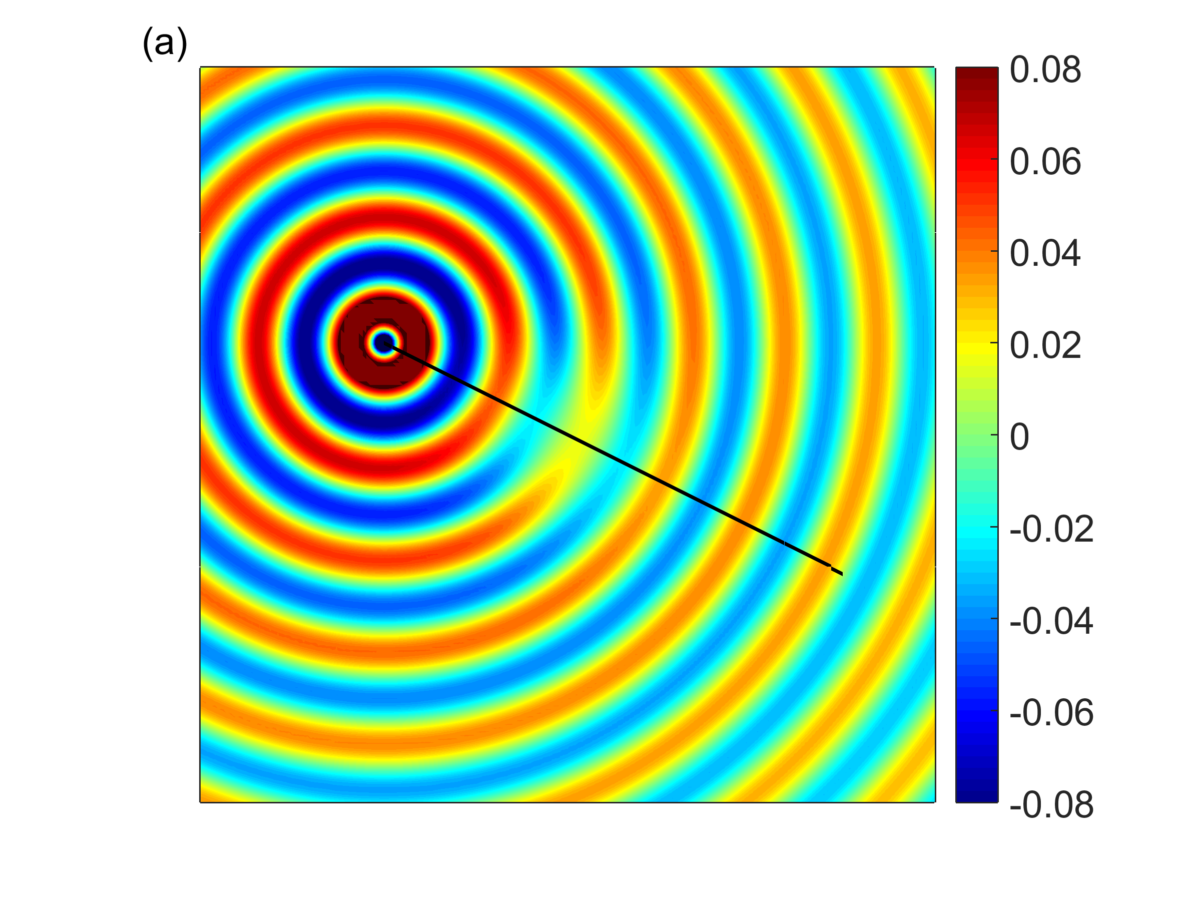 Figure 1
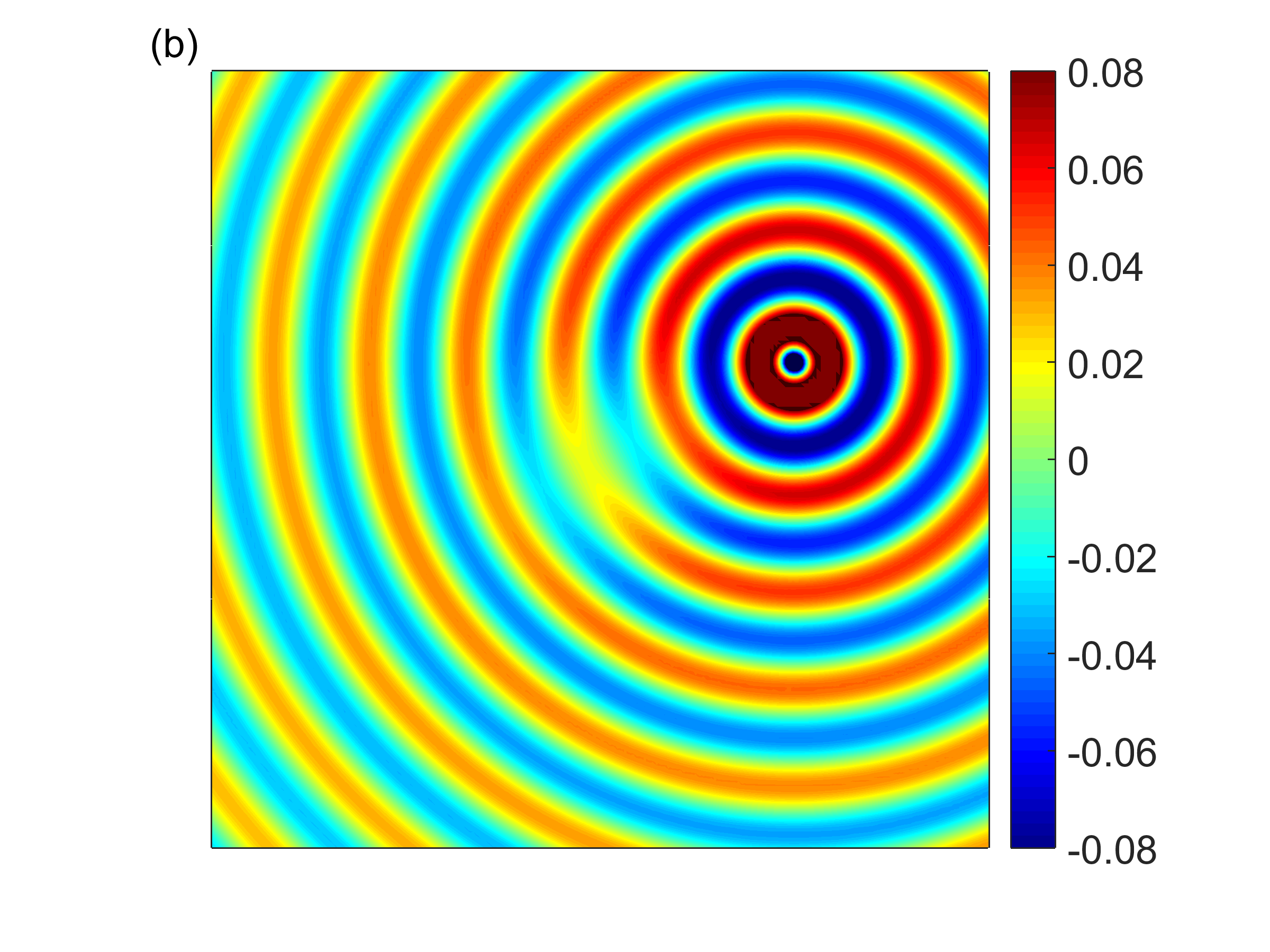 Figure 1
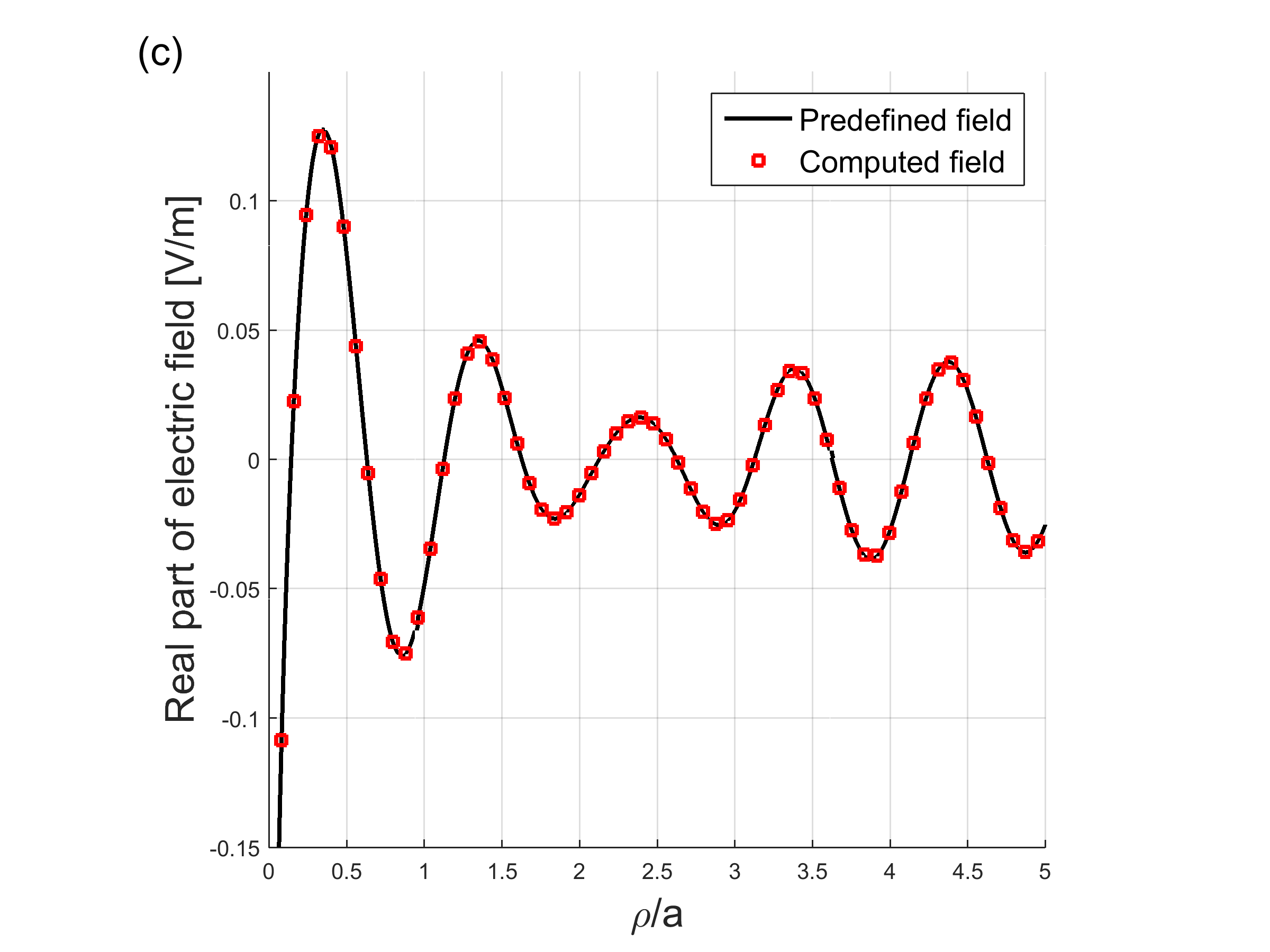 Figure 1
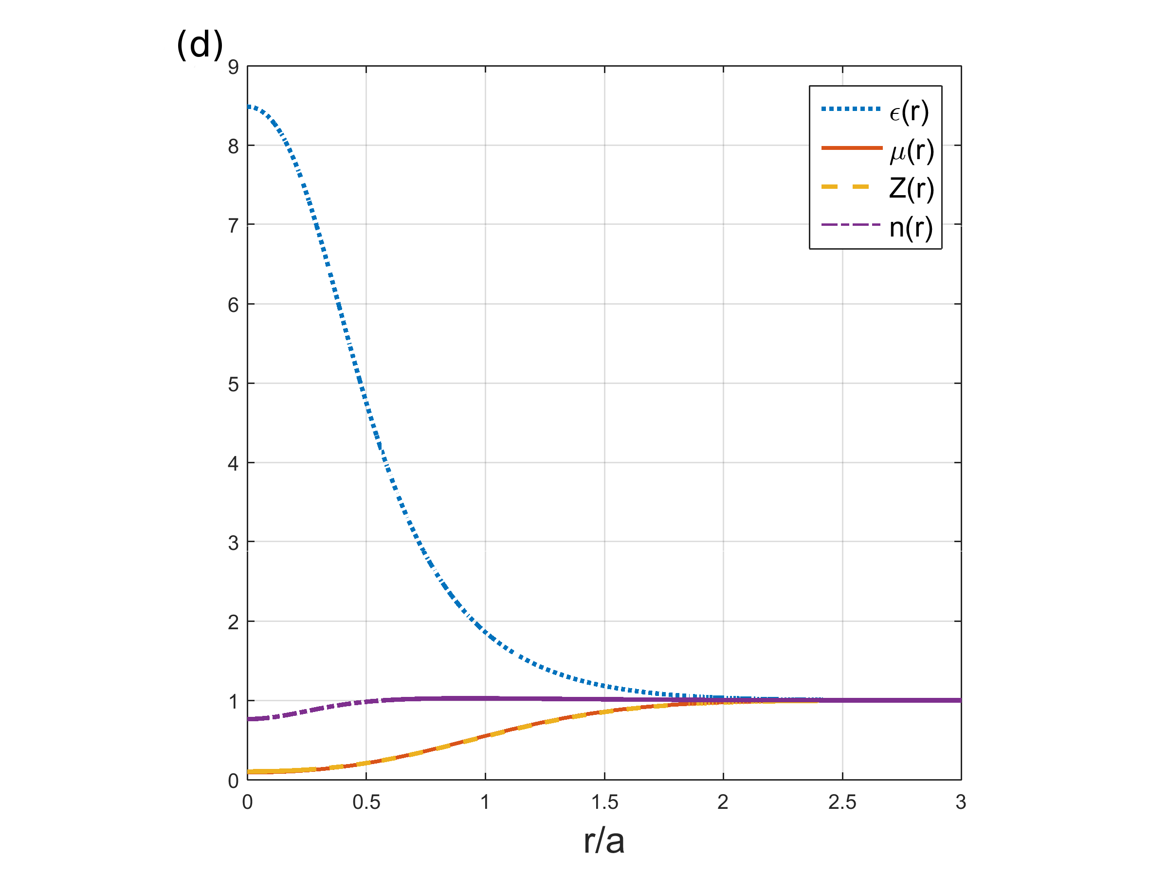 Figure 1
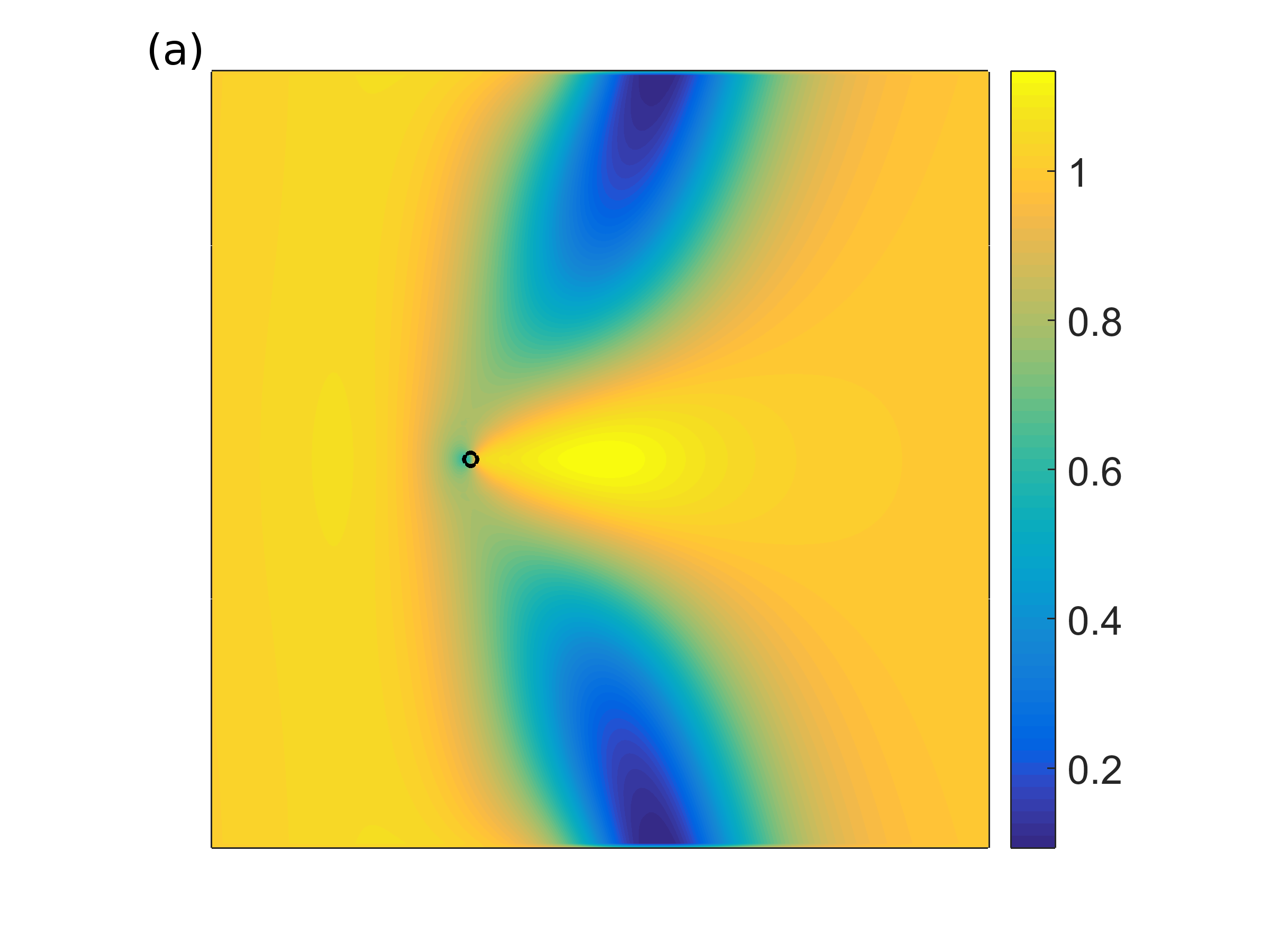 Figure 2
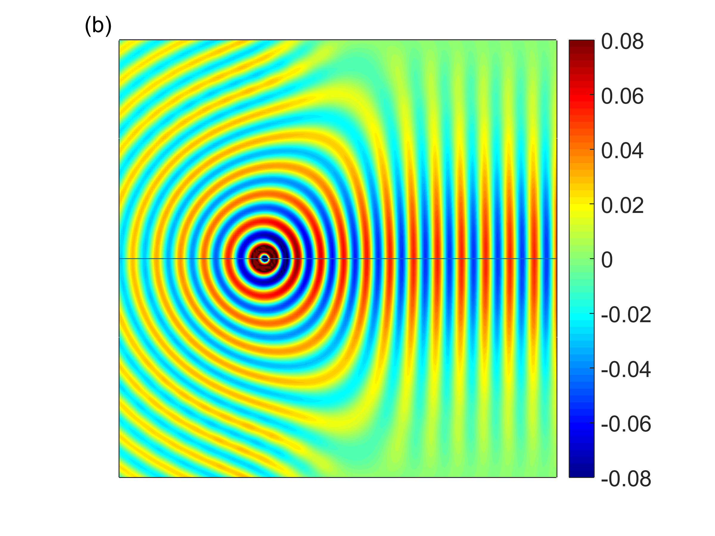 Figure 2
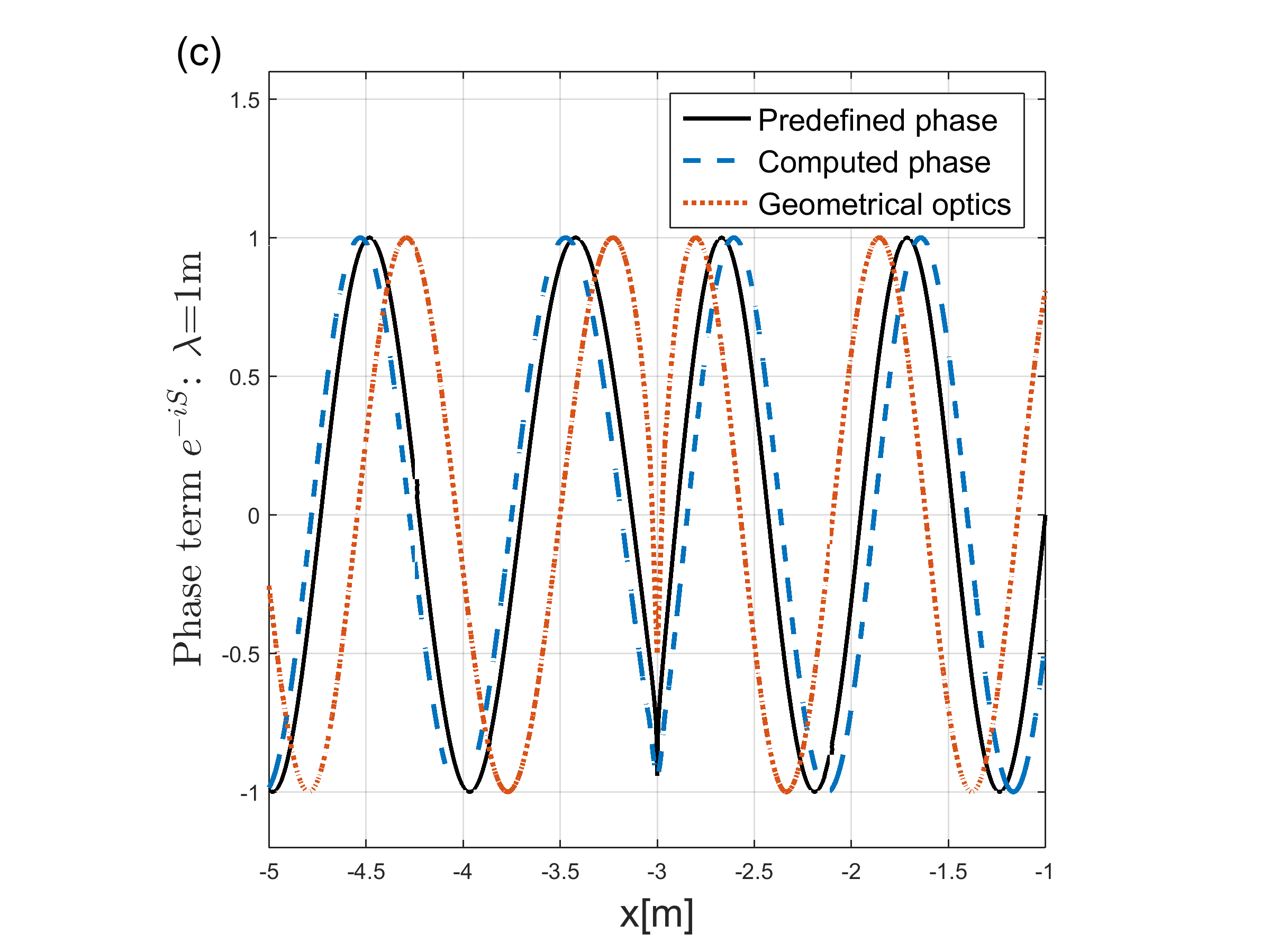 Figure 2
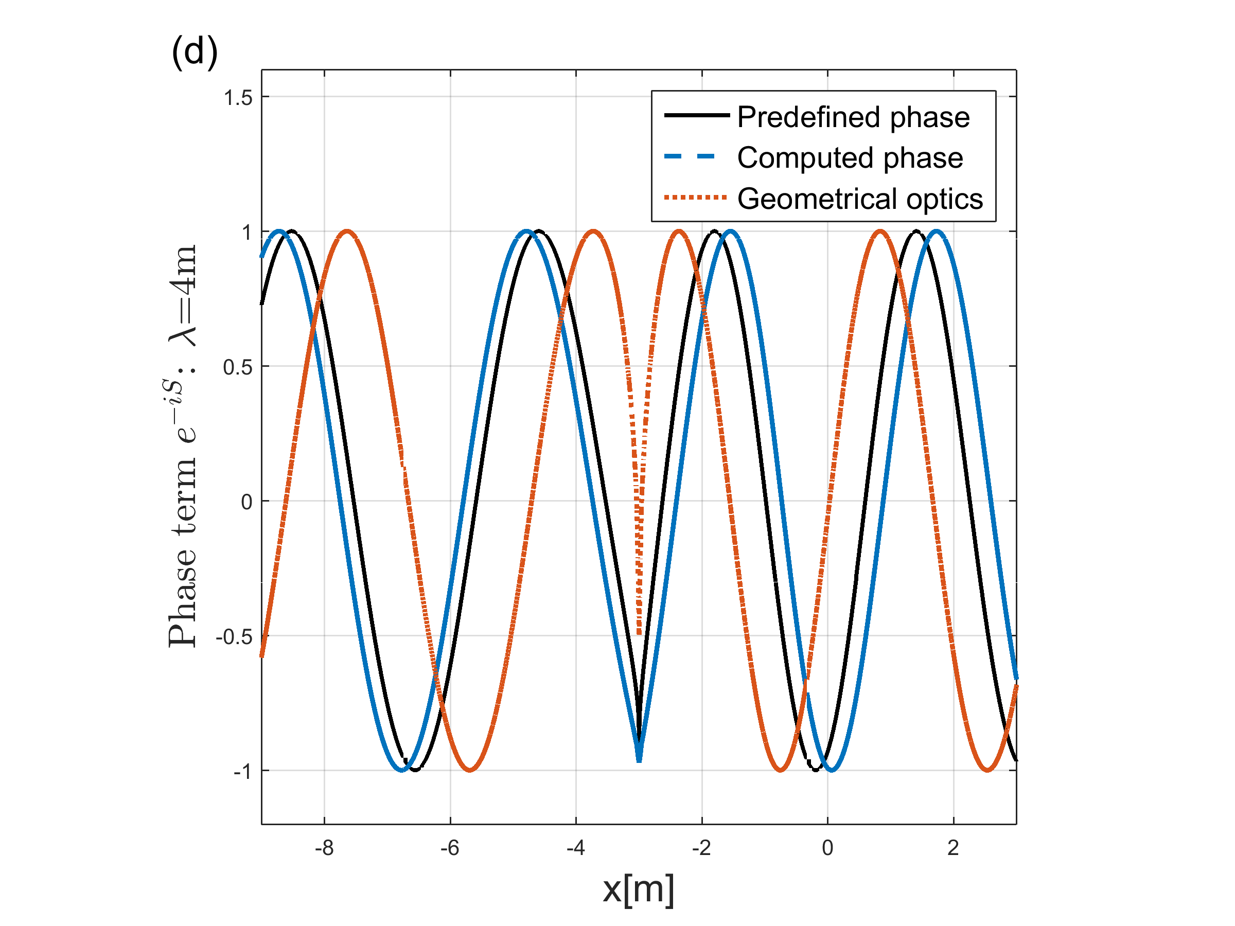 Figure 2
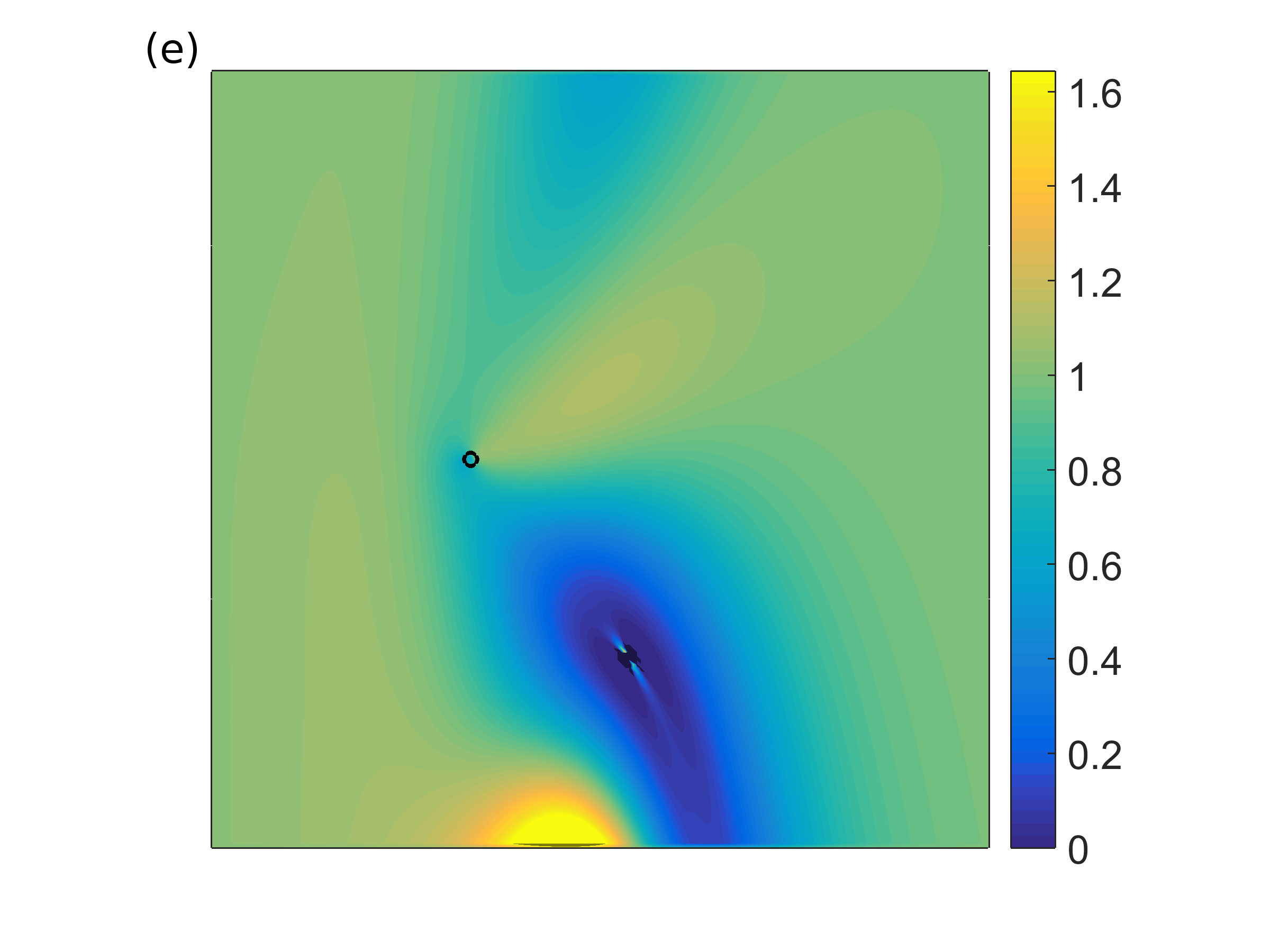 Figure 2
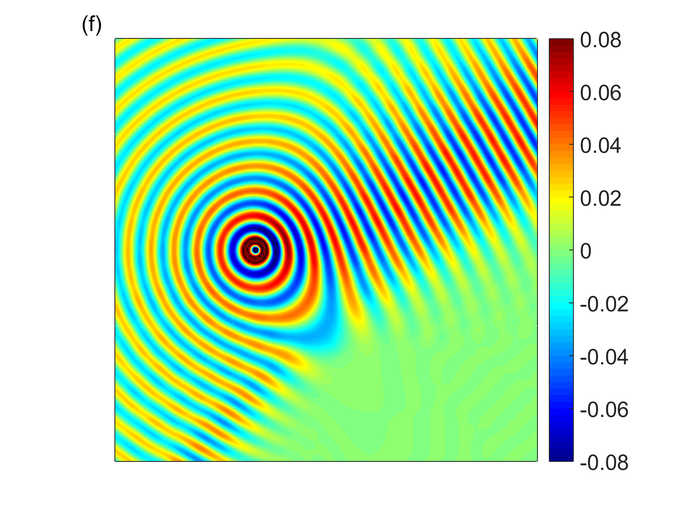 Figure 2
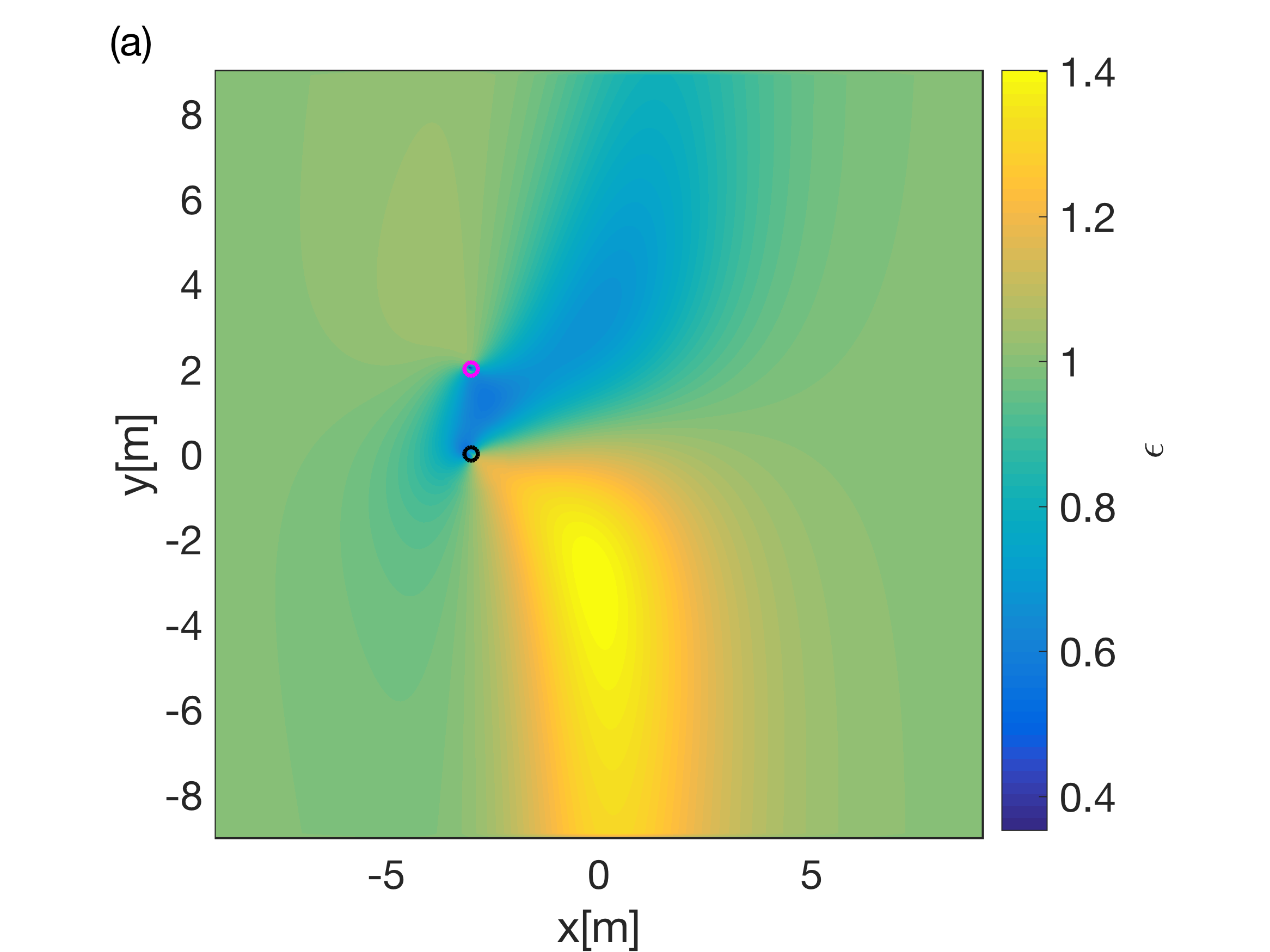 Figure 3
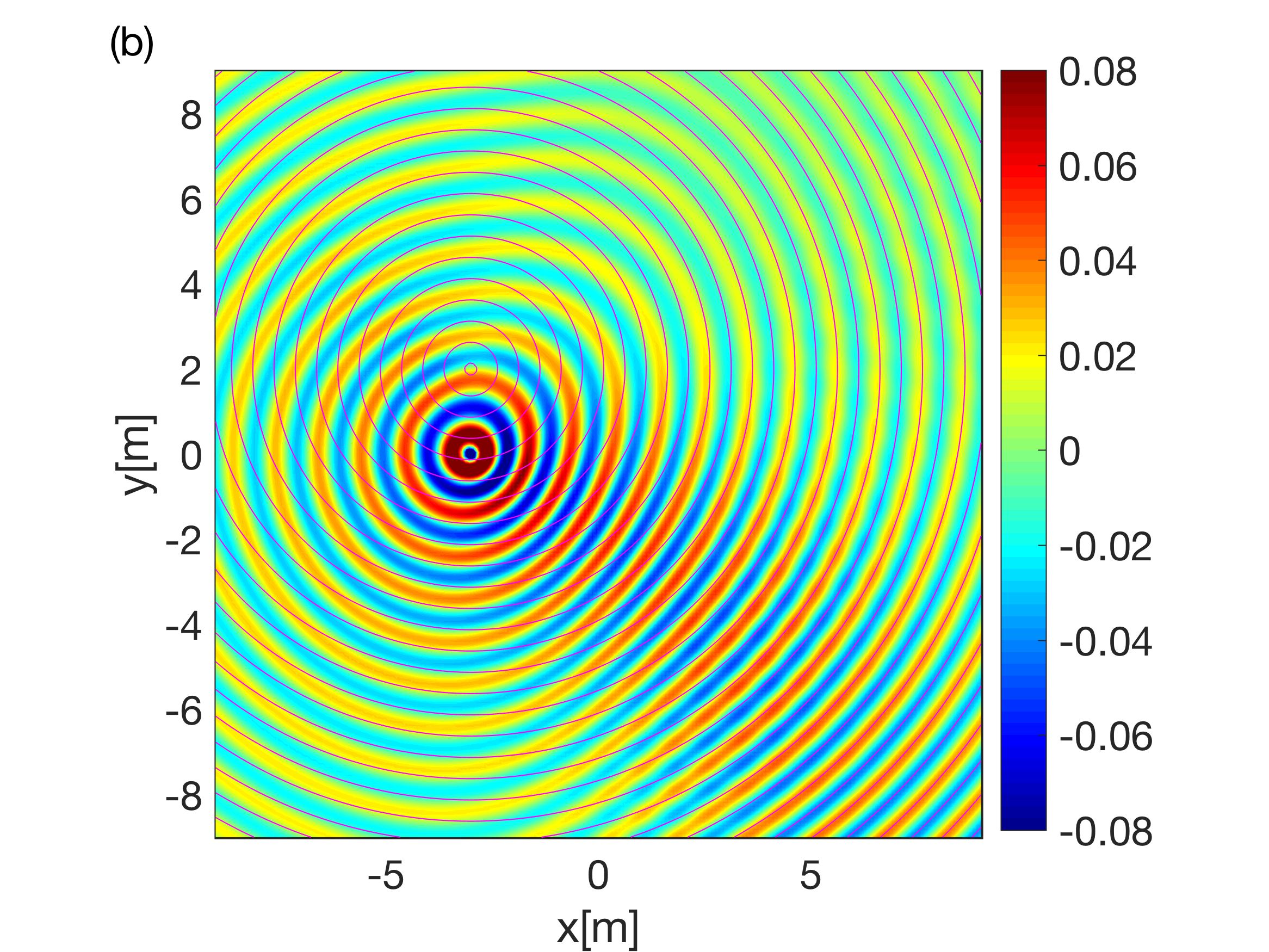 Figure 3
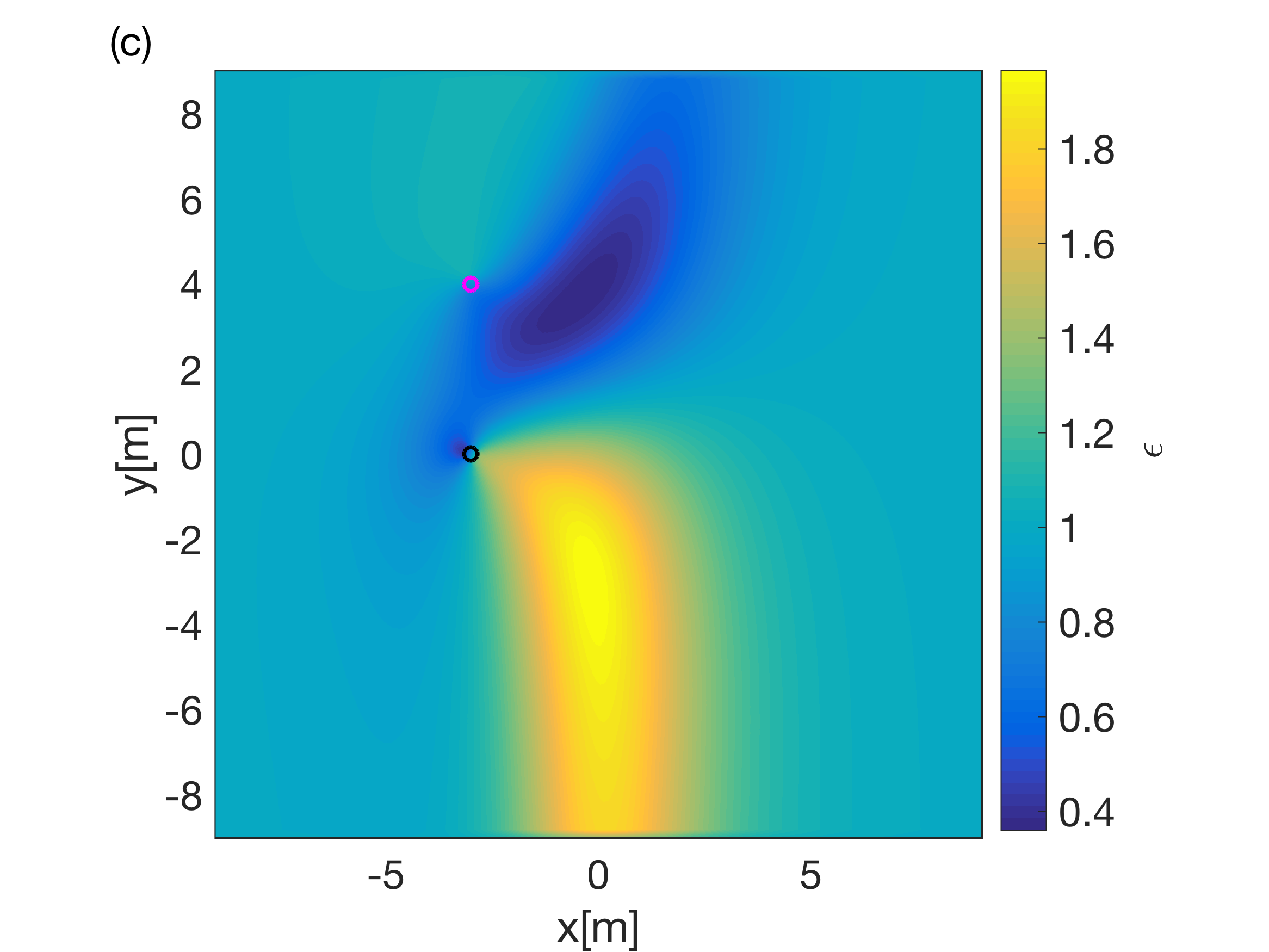 Figure 3
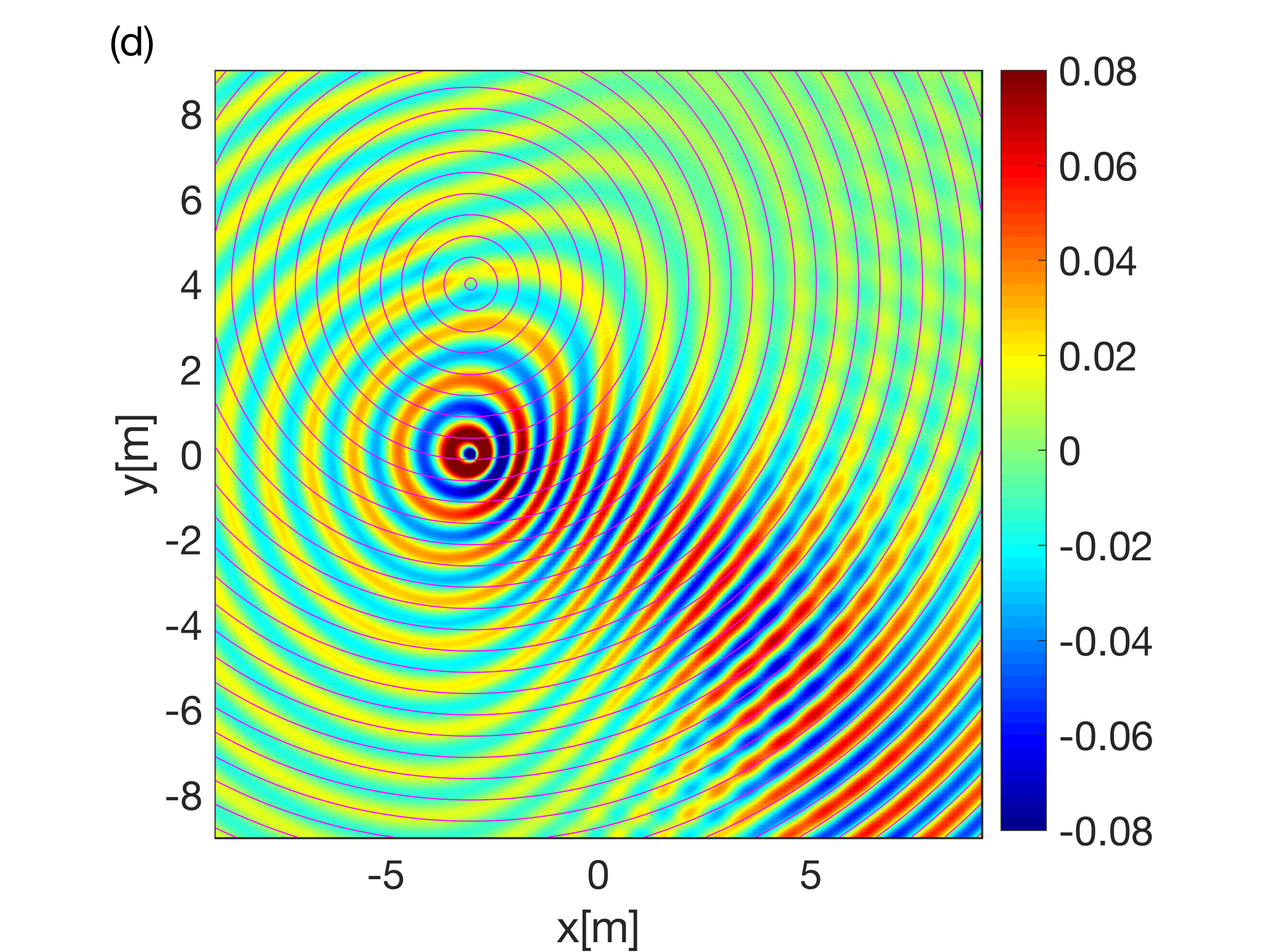 Figure 3
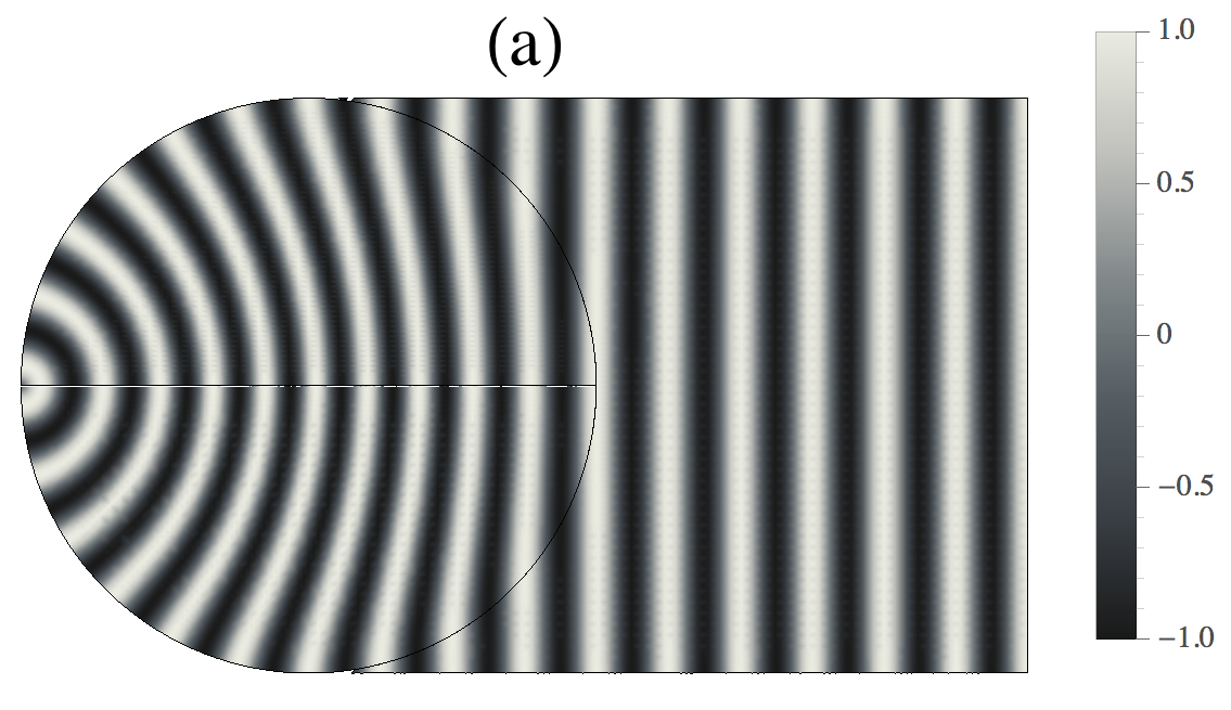 Figure 4
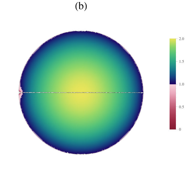 Figure 4
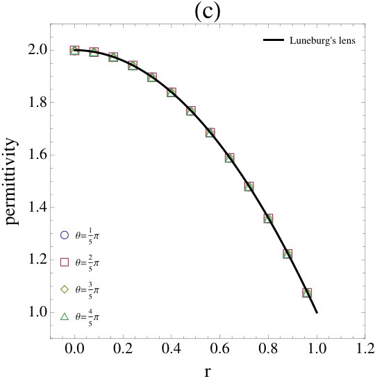 Figure 4
Peer Reviews
No public reviews on file for this paper yet. If you reviewed it on a platform where reviews are public (OpenReview, ICLR, NeurIPS, ICML), you can paste yours below so the community can read it here.
Videos
No videos yet. Explain this paper in a talk, walkthrough, or lecture? Add one.
Direct manipulation of wave amplitude and phase
through inverse design of isotropic media
Yangjié Liu (刘\CJKkern泱\CJKkern杰)
Antennas Group, School of Electrical Engineering and Computer Science, Queen Mary University of London, 327 Mile End Road, E1 4NS, England, United Kingdom
Faculty of Physics and Electronic Science, Hubei University, 368 Youyi Road, 430062 Wuchang District, Wuhan P. R. China
B. Vial
Antennas Group, School of Electrical Engineering and Computer Science, Queen Mary University of London, 327 Mile End Road, E1 4NS, England, United Kingdom
S. A. R. Horsley
Department of Physics and Astronomy, University of Exeter, Stocker Road, Exeter, EX4 4QL, England, United Kingdom
T. G. Philbin
Department of Physics and Astronomy, University of Exeter, Stocker Road, Exeter, EX4 4QL, England, United Kingdom
Y. Hao
Antennas Group, School of Electrical Engineering and Computer Science, Queen Mary University of London, 327 Mile End Road, E1 4NS, England, United Kingdom
(accepted 7 April, proofread 14 June, compiled )
Abstract
In this article we propose a new design methodology allowing us to control both amplitude and phase of electromagnetic waves from a cylindrical incident wave. This results in isotropic materials and does not resort to transformation optics or its quasi-conformal approximations. Our method leads to two-dimensional isotropic, inhomogeneous material profiles of permittivity and permeability, to which a general class of scattering-free wave solutions arise. Our design is based on the separation of the complex wave solution into amplitude and phase. We give two types of examples to validate our methodology. 111Submitted to New J. Phys. 28 Dec-2016, initial decision received 23 Feb, deposited 21 Jan in arXiv (https://arxiv.org/abs/1701.06021v1), NJP-106316.R1 resubmitted 14 March, accepted 7 April 2017 as Manuscript # aa6c0c (http://iopscience.iop.org/article/10.1088/1367-2630/aa6c0c/), 6 July published online, 3 Aug 2017 updated in arXiv (https://arxiv.org/abs/1701.06021v2).
pacs:
41.20.Jb Electromagnetic wave propagation. 42.25.-p Wave optics. 02.30.Zz Inverse problems. 02.60.Cb Solution of equations.
I Introduction
Transformation optics (TO) has proved as a remarkable design tool to engineer materials which are capable of manipulating waves in an arbitrary manner Pendry (2006); Leonhardt (2006a, b); Leonhardt and Philbin (2010); Post (1962). It yields material parameters when wave behaviours are predefined by coordinate deformation, the wave remaining impedance-matched to the virtual space (usually the air). However, this method or its derivatives such as quasi-conformal mapping are limited to problems with a “mother” design required in a virtual space. What remains less explored is the vast space of inhomogeneous isotropic media Leonhardt and Philbin (2010); Schmiele et al. (2010), especially those not of transformation media. While the material parameters derived from transformation optics are generally anisotropic, the quasi-conformal transformation can be applied to reduce the anisotropicity Li and Pendry (2008) and other numerical techniques can also be applied to achieve other types of inverse isotropic design Chang et al. (2010); Liu et al. (2013); Piggott et al. (2015); Ginis et al. (2016). Thus the material parameters shall be more readily manufactured if we can design isotropic materials without resorting to quasi-conformal approximations Li and Pendry (2008).
Generally a different approach to design the isotropic, graded index medium for light is demandedLeonhardt and Tyc (2009); Leonhardt and Philbin (2010). We are thus tempted to look into the analytic relation between the wave solution and material parameters, in the hope of gaining some new insight about the design philosophy of tackling the optical inverse problem in inhomogeneous media. This approach will generally result in 2D graded index profiles of media, other than only 1D graded indices of refraction Dalarsson and Tassin (2009).
In this paper we will demonstrate a method for designing graded-index, isotropic material profiles of an optical inverse problem which give scattering-free wave solutions Vial et al. (2016). We will start from the wave equation Philbin (2014) and show the otherwise implicit relation between a reflection-free wave solution in polar form and its corresponding material profiles. This is an alternative method to compute material parameters other than transformation optics, and circumvents the trail-and-error way to guess parameters.
We emphasise that our theory is a general approach to designing material profiles for non-reflective electromagnetic waves, and should be extendable to vectorial, three-dimensional cases despite the mathematical complication. For simple illustration, we restrain our investigation in this paper to two-dimensional case with linear polarisations Kim and Park (2013). The merit of the analysis applied here lies in its simplicity to design the material profile without resorting to numerics. A remark to note is that our design profiles of material are real-valued, which surprisingly supports reflection-less waves for certain incident waves. This contrasts with the complex material profiles that work for a single angle of incidence 222Taking with at infinity and plugging this into the wave equation of no source (2), one reads off the corresponding permittivity. .
The structure of the paper is as follow. The methodology for designing material profiles to achieve predefined amplitude or phase will be given in Sec. II. The example material profiles in this paper are designed for two types of wave solutions: 1) a spatial-modulating wave from a point source (Sec. III), which keeps its phase as if in free space; 2) a wave transiting from a point source to another phase (Sec. IV). Therefore we demonstrate how one can control the wave front – maintaining it or varying it at our will, respectively. Sec. V remarks about the condition when the wave equation Eq. (2) aligns with exact geometrical optics Philbin (2014). Sec. VI concludes the article.
II Methodology
We start from vectorial Maxwell equations for 2D isotropic, inhomogeneous and passive medium, where the relative permittivity and permeability are real, spatial-varying functions Born and Wolf (2009). We aim to design the material profiles which both reduce to unity in the far region (). The electromagnetic wave in two-dimensional case, can be decoupled into two separate scalar solutions: transverse electric (TE) and transverse magnetic (TM) components. For TE component, we represent its scalar parts in frequency domain, in polar form of real amplitude and phase as 333To be compatible with the model setup in COMSOL simulation, we choose the engineering time harmonic convection .:
[TABLE]
where the TE waves is composed of amplitudes and phase . Explicitly the TE wave equation is written as
[TABLE]
where with the light velocity in vacuum. Eq. (2) will be the main wave equation we use in this article. The magnetic field for TE mode is given in terms of the electric field by Faraday’s law of induction, when the electric field is known:
[TABLE]
As for TM polarisation and the solution for fileds, similar results hold when the permittivity and permeability are swapped.
In this article, we will focus on the TE wave in Eq. (2). From Eqs. (1) and (2) we obtain the equivalent of the wave equation in terms of amplitude and phase
[TABLE]
We now analyse wave manipulation when it traverses the inhomogeneous medium. The material profiles are always designed to reduce to one in the far region. We choose an incident wave vector , in which is its unit vector. We interpret the wave dynamics as a system where an incidence wave from the source impinges the whole medium from one side, then interacts with the non-trivial graded index medium in the middle. Finally it exits to the other side the medium (air) with no scattering. The gradient of the phase is written as a sum of incident wave vector and the gradient of an unknown function :
[TABLE]
Then Eq. (5) can be written as Poisson’s equation, with playing the role of the scalar potential. This can be solved in the same way as the equivalent problem in 2D electrostatics, where (cf. pp4-7Liu (2014)). Therefore can be given as
[TABLE]
where . This integral physically indicates that the incident wave vector and spatially dependent amplitude serve as the source of .
An interesting case occurs when vanishes everywhere, i.e. the wave not only exits the medium as the same incident wave, but also keeps its phase unchanged throughout space with respect to the incident wave, even inside the medium. This occurs when the source term vanishes in Eq. (7). We shall term the medium an invisible material for a certain incidence wave and its examples will shown in Sec. III. In another case when does not vanish throughout the medium, the incidence wave shall withstand a non-zero phase change in the middle of medium, and then outputs as a different wave. This medium shapes one incidence wave into another. We shall show in Sec. IV two instances of such a type of conversion medium, which transforms a cylindrical wave into others.
II.1 Controlling the wave amplitude
Now we demonstrate our method to design a medium, which controls the wave amplitude generated from a localised current source in free space and leaves the wave phase unchanged as that in free space.
Generally in a graded index medium the wave equation with source in frequency domain is
[TABLE]
similar to Eq. (2). In free space air, Eq. (8) reduces to
[TABLE]
in which is the reference wave solution resulting from a source . The form of Eqs. (8) and (9) includes the special case of planar wave of incidence, i.e. the source term is infinite away and thus equivalent to zero.
Supposing the source is positioned in a bounded region in air, the source-free wave equation Eq. (2) actually still stands all over the field region except in the source region. This means that we can disregard the source term in Eqs. (8) and (9), and still use Eqs. (4) and (5) derived from Eq. (2) 444The general situation when the source sits in non-trivial region where material parameters are not unity, is far more complicated and beyond scope of this article. . We want to control the wave amplitude as
[TABLE]
where is the modulation factor determined by the designer with respect to the reference wave solution, i.e. . The modulation factor can be arbitrary function as long as it reduces to unity in far field. Then substituting Eq. (9) into Eqs. (4)-(5) we have in source-free region
[TABLE]
This includes the special case in air where the reference wave solution in source-free region follows
[TABLE]
We then solve the material profiles in Eqs. (II.1) and (12) as
[TABLE]
by making use of Eqs. (10) and (13). Here by definition is positive. Note that this solution is obtained under the condition that the source sits in the far field region of . If the source is put in region , the scattering-free effect of the designed material will no longer hold. The wave amplitude in the whole domain can be designed in an arbitrary manner 555Due to our condition that the current source sits in trivial region, we cannot control the wave amplitude in the source region. in the central region when . The physical constraint on is that it should smoothly vary within space in order to give a finite range for material profiles in Eqs. (15) and (16). The function can vary with a sharper resolution than the wavelength, although resulting in a larger value range for the requisite material profile . We shall give an example for this method to control the wave amplitude in Sec. III where the source is chosen as a point source in 2D space.
II.2 Controlling the phase
We can also control the phase function of the wave. If a given phase distribution is desired, we can use Eq. (6) to find the requisite material parameters. We solve for wave amplitude and material parameters, starting from Eq. (5) and write it compactly by defining . One thus has
[TABLE]
Then we may write
[TABLE]
Above is a unit perpendicular vector to and is an unknown factor in front of 666Note that the variable as the factor before the perpendicular vector is actually not arbitrary as it might appear at the first sight. The reason not being so is two-fold: 1) the requirement that material parameters reduce to unity prevents us from exploiting the freedom; 2) moreover, is restrained in order to compliment the former term on the right side of Eq. (18) into a gradient. Therefore it cannot be arbitrary function of and . Thus Eq. (18) is an integrability problem to solve. Once is known, one can design the wave amplitude and the permeability becomes known. . Though generally the partial differential equation for could be solvable by numerics with an appropriately chosen boundary condition, we choose to approximate the solution as Eq. (19) because it lends a simpler closed form in material parameters.
For simplicity, in non-magnetic case () we can approximate the permittivity in an analytic form by substituting Eq. (19) into Eq. (4), and then one obtains
[TABLE]
The first leading term in Eq. (20) is essential from the geometrical-optical eikonal equation. The rest terms represent the high order correction to give a more accurate design to account for wave optics than for geometrical optics. Note that generally no longer equals as the module of wave vector varies through the inhomogeneous medium. One can also predetermine magnetic material and then obtain a different permittivity , in which the same phase as nonmagnetic material is achieved. We will give two examples of wave front conversion design in Subsec. IV.1.
III Invisible material for a point source
Apart from planar propagation Vial et al. (2016), a simple incident wave in 2D case is the cylindrical wave from a point source (a line of source in 3D space). As an example to apply the method in Sec. II.1, in the same material Eqs. (15) and (16), the amplitude of a cylindrical wave is also controllable. In this case the reference wave in Eq. (9) becomes the Green function for a point source, which is written as
[TABLE]
where are respectively, the first and the second kinds of Bessel functions of zeroth order and the cylindrical phase is defined as . The controlled amplitude is thus
[TABLE]
As an example we indicate where are parameters. The wave solution and the scattered wave from a point source in such a reflectionless medium is plotted in Fig. 1(a-b), respectively. It is noted that our designed material Eqs. (15) and (16) plotted in Fig. 1(d) works for any point source positioned in free space region. The excellent comparison between simulation and predefined wave field value along a line segment in Fig. 1(a) is demonstrated in Fig. 1(c).
Note that in fact, our designed material in Eqs.(15) and (16) works for any current source sitting anywhere but the non-trivial region where factor strongly deviates from unity, i.e. the designed medium independent on the source modulates the field from any source, which causes no scattering throughout the space. Hence this is actually another class of invisible media made of positive isotropic material similar to Tyc et al. (2014) but possesses zero phase delay, although no room to hide any object in this case. Generally, the rotational symmetry of is not a compulsory condition and a more general profile still works as an invisible material, as long as the material profiles are continuously second-order derivable.
For summary of Sec. III, we give an examples of reflection-less wave from a point source, which enters the medium from one side and recovers to its initial wave shape at the other side.
IV Phase conversion material
In this Sec., we will design material profiles which convert an incident wave of one phase into another. The examples are given in Subsec. IV.1. The first converts a cylindrical wave to a planar one, and the second to another shifted cylindrical wave, as if from an illusional point source. In Subsec. IV.2 we also validate our method to control the phase, reproducing Lüneburg lens as a special case.
IV.1 Wave front conversion - from a cylindrical wave to other phases
We apply the general formula Eq. (20) derived in Subsec. II.2 to design a conversion material, which transfers a cylindrical wave from a point gradually to another wave of phase. The phase of the wave in such a medium can be written as
[TABLE]
Here is the incoming wave phase, the output wave phase and is a transition function varying from 0 to 1 as increases 777We choose only x dependence for simplicity. . In free parameter can be tuned to control how quickly the phase varies from cylindrical (the incident wave phase is cylindrical according to Eq. (III)) to planar. Then we obtain immediately the permittivity profile from Eq. (20).
First we choose the output beam to be a wave of planar phase 888Reciprocality of wave equation implies that one could also choose the output to be a cylindrical wave. However, this will give a wave picture of inevitable scattering (not shown in the paper).
[TABLE]
in which is the angle between incident wave vector and x axis. Numerical wave simulation in Fig. 2 shows that one can design the conversion medium not only for normal incidence angle depicted in Fig. 2(a-b), also for an oblique one as in Fig. 2(e-f). For the case of normal incidence, we compare the computed phase along x axis (see black line in Fig. 2 (b)) from simulation with the predefined phase in Eq. (24). In Fig. 2 (c-d) the phase from our design differs only by a small delay, and the phase from geometrical optical design is more errant from predefined phase. Thus our method based on wave optics yields a more accurate medium than from geometrical optics.
Secondly, we also design a beam shifting medium similar to Gallina et al. (2010) where the output wave phase is chosen to be a laterally-shifted cylindrical phase from :
[TABLE]
From simulation, the designed profiles of permittivity in Fig. 3(a, c) transfers the wave from the point source (in black) to that from the shifted one (virtual, in magenta). The phase of the output beam from the point source converts to that of a shifted beam, which are indicated by magenta contours in Fig. 3(b, d).
IV.2 An example to illustrate the validation of phase conversion materials
As the Lüneburg lens focuses a planar wave into a single point at its edge, we naturally wonder if this is recoverable via our design formula Eq. (20). In the case of planar-wave illumination, we will retrieve the analytic phase distribution (see Fig. 4(a)) from ray-tracing Leonhardt and Philbin (2010), and obtain an almost identical profile of permittivity as Lüneburg lens, depicted in Fig. 4(b-c). Further detail is included in Appen. A. We are therefore assured that this method is reliable.
IV.3 Metamaterial implementation
In order to verify feasibility of our design methodology, we briefly discuss a possible metamaterial implementation here. Our previous implementation and simulation already verify our design methodology Vial et al. (2016)(Sec. IIC therein) and thus we shall not repeat in detail. We propose to use two kinds of materials (SiC silicon carbide and KBr potassium bromide with permittivity and at ), which are hosted in air to arrange as small-rod arrays. One can compute which requires the rod-sizes from homogenisation theory (Maxwell-Garnett formula). In engineering realisation, the material loss could play a role and weaken the wave amplitude than predicted Vial et al. (2016). Note that our proof-of-concept design is de facto based on lossless material parameters, which can be taken into account to give rise to an more accurate design scheme.
V Deviation from exact geometrical optics
A natural question to ask is whether our method aligns with geometrical optics Philbin (2014). For TE wave, we find that geometrical optics stands when
[TABLE]
such that Eq. (4) recovers the eikonal equation Philbin (2014)
[TABLE]
if one defines effective refractive index . Therefore it is easy to find that both our examples in Fig. 1 are deviant from the condition of exact geometrical optics 999see Eq. (29.4) of Leonhardt and Philbin (2010). Moreover for TE wave, Eq. (28) will stand for all frequency, if a different wave equation
[TABLE]
can be postulated, if we are able to allow some special material response which contributes to the last term above (cf. Sec. 5 of Philbin (2014)).
VI Conclusion
In summary, this paper extends our method Vial et al. (2016) to design for scattering-free wave amplitude or phase in isotropic, heterogeneous medium and focus on manipulating cylindrical wave in 2D case. This elegant analytic method inversely designs the material parameters in a different route compared with transformation optics Leonhardt (2006a); Pendry (2006). We give two types of examples to demonstrate our design scenario: an invisible material and a wave front conversion medium both for a point source. This method generally works for monochromatic frequency and is highly narrow-band limited. Our design method and and simulation verification are given for 2D TE wave for isotropic medium, which can be extended to the TM wave, and even 3D case 101010See Potvin (2015) for a mathematical approximation in 3D case. . Extension to anisotropic materials is also possible. Moreover, our method could camouflage a certain amount of scattering wave, although the inverse problem for a scattering wave should be far more complicated and challenging. We hope this method can shed some light on how to design graded-index materials in order to keep or change the phase of a cylindrical wave.
Acknowledgements.
We are supported by the Engineering and Physical Sciences Research Council (EPSRC) of UK [grant number EP/I034548/1]. L Y benefits from LMS-EPSRC Durham Symposium 104, LMS Caring Supplementary Grant [Ref. CC-15/16-09] and Antennas group travel grant [EECSRC2/4a], and wants to thank Patrick Bradley, Flynn Castle and Fang Yanlong for inspiring conversations to improve this manuscript. This article is supported by the EECS Open Access group and Queen Mary Library ().
Appendix A Derivation to recover Luneburg lens
In Subsection IV.2, we recover the permittivity profile of Lüneburg lens by taking the phase function for planar incidence wave illuminated from right side of the lens. Here is the detailed derivation to retrieve the phase information. While one can generally relies on numerical method of solving Hamilton’s equations to retrieve the phase information, we choose to analytically solve the phase distribution for two dimension as follows, which shall be easily extended to a three dimensional case. Firstly, Lüneburg lens profile in dimensionless unit is written as
[TABLE]
And we illuminate a planar wave from straight line and focus it into its focus at . We shall use complex coordinates to simplify our derivation. What remains is to write explicitly the phase for each point inside the unit circle, since the phase outside it is just a planar wave phase. For each point , it shall fall on a specific ray penetrating the circle at two intersection points and , sequentially. In complex coordinates , any tray inside Lüneburg lens can be written as
[TABLE]
And its two joint points with the unit circle are represented as and , where serves as the parameter inside the circle.
Next we solve and as functions of . Substituting the coordinates of the three points above into Eq. (31), one can obtain
[TABLE]
and
[TABLE]
The later two equations can be combined into a quartic equation
[TABLE]
With the physical solution in mind, one can solve
[TABLE]
[TABLE]
[TABLE]
Note that needs to be in the second quadrant according to Eqs. (32) and (33).
Now we are ready to write out the phase of an arbitrary point as
[TABLE]
knowing that it composes of the sum of phase accumulated outside and inside the lens. After a straightforward derivation 111111The inverse tangent function is defined following ArcTan in Wolfram Mathematica 10, such that it gives the the right angle of among four quadrants.
[TABLE]
The interval of parameter dictates the physical solutions of to be
[TABLE]
Note that becomes peculiar when and we can write the phase
[TABLE]
Substituting the full phase Eq. (43) depicted in Fig. 4(a), into our formula of permittivity Eq. (20)
[TABLE]
we calculate the designed profile as Fig. 4(b-c) shows. The designed permittivity goes below unity near the source point , which is due to the fact that the phase near source point is undefined [cf. Fig. 4(b)]. Despite that, it is clear that our method successfully reproduces that of Lüneburg lens [see Fig. 4(c)].
The reference list from the paper itself. Each links out to its DOI / PubMed record.
- 1Pendry (2006) J. B. Pendry, Science 312 , 1780 (2006) . · doi ↗
- 2Leonhardt (2006 a) U. Leonhardt, Science 312 , 1777 (2006 a) . · doi ↗
- 3Leonhardt (2006 b) U. Leonhardt, New Journal of Physics 8 , 16 (2006 b) . · doi ↗
- 4Leonhardt and Philbin (2010) U. Leonhardt and T. Philbin, Geometry and Light : The Science of Invisibility , Dover Books on Physics (Dover Publications, Inc., Mineola, N.Y., 2010) p. 278.
- 5Post (1962) E. J. Post, Formal Structure of Electromagnetics–General Covariance and Electromagnetics (North-Holland Publishing Companuy, Amsterdam, 1962).
- 6Schmiele et al. (2010) M. Schmiele, V. S. Varma, C. Rockstuhl, and F. Lederer, Physical Review A 81 (2010), 10.1103/Phys Rev A.81.033837 . · doi ↗
- 7Li and Pendry (2008) J. Li and J. B. Pendry, Phys. Rev. Lett. 101 , 203901 (2008) . · doi ↗
- 8Chang et al. (2010) Z. Chang, X. Zhou, J. Hu, and G. Hu, Opt. Express 18 , 6089 (2010) . · doi ↗