Covariance Functions for Multivariate Gaussian Fields Evolving Temporally over Planet Earth
Alfredo Alegr\'ia, Emilio Porcu, Reinhard Furrer, Jorge Mateu

TL;DR
This paper develops new flexible covariance functions for multivariate Gaussian fields evolving over time on spherical surfaces, crucial for modeling climate and ocean data across the globe.
Contribution
It introduces a novel family of matrix-valued covariance functions for spherical space-time data, extending Gneiting models and latent dimension approaches.
Findings
Models effectively capture space-time dependencies on the sphere.
Proposed covariance functions improve prediction accuracy.
Application to climate data demonstrates practical utility.
Abstract
The construction of valid and flexible cross-covariance functions is a fundamental task for modeling multivariate space-time data arising from climatological and oceanographical phenomena. Indeed, a suitable specification of the covariance structure allows to capture both the space-time dependencies between the observations and the development of accurate predictions. For data observed over large portions of planet Earth it is necessary to take into account the curvature of the planet. Hence the need for random field models defined over spheres across time. In particular, the associated covariance function should depend on the geodesic distance, which is the most natural metric over the spherical surface. In this work, we propose a flexible parametric family of matrix-valued covariance functions, with both marginal and cross structure being of the Gneiting type. We additionally…
Click any figure to enlarge with its caption.
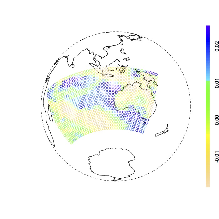 Figure 1
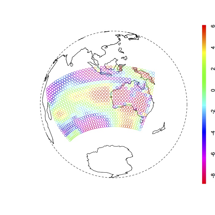 Figure 2
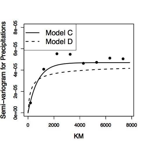 Figure 3
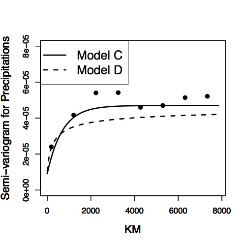 Figure 4
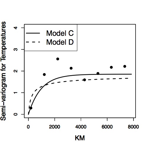 Figure 5
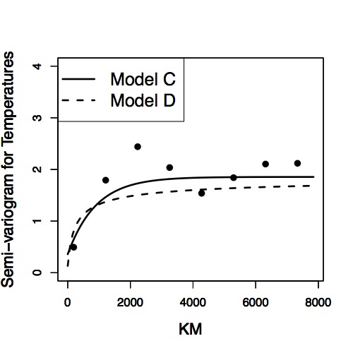 Figure 6
 Figure 7
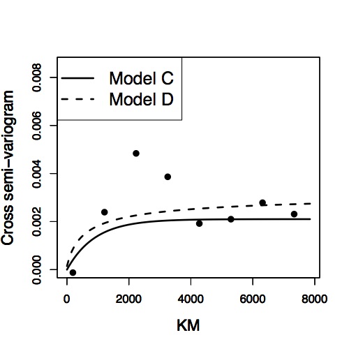 Figure 8
| Function | Parameters restriction |
|---|---|
| , | |
| , | |
| , , | |
| , |
| Function | Parameters restriction |
|---|---|
| , , | |
| , | |
| , , |
| Model A | 1.85 | 0.28 | 102 | 102 | 102 | 11.88 | ||
| Model B | 1.84 | 0.28 | 2602 | 2602 | 2602 | 22.58 | ||
| Model C | 1.85 | 0.28 | 2901 | 2245 | 2901 | 22.92 |
| Model D | 1.38 | 47133 | 30805 | 41.36 | 4.03 | 1.66 |
| Log-CL | |||||
|---|---|---|---|---|---|
| Model A | 5.79 | 0.27 | 2.07 | 1.21 | 1.52 |
| Model B | 5.80 | 0.13 | 1.62 | 0.67 | 1.02 |
| Model C | 5.81 | 0.11 | 1.61 | 0.62 | 0.93 |
| Model D | 5.81 | 0.11 | 1.84 | 0.63 | 0.62 |
| Notation | Description |
|---|---|
| Positive definite matrix-valued () functions on . | |
| Continuous, bounded and stationary elements of . | |
| Continuous, bounded and Euclidean isotropic elements of . | |
| Continuous, bounded and geodesically isotropic elements of . | |
| Elements in being, continuous, bounded, geodesically | |
| isotropic in the spherical variable and stationary in the Euclidean variable. |
Peer Reviews
No public reviews on file for this paper yet. If you reviewed it on a platform where reviews are public (OpenReview, ICLR, NeurIPS, ICML), you can paste yours below so the community can read it here.
Videos
No videos yet. Explain this paper in a talk, walkthrough, or lecture? Add one.
\AtAppendix\AtAppendix\AtAppendix
Covariance Functions for Multivariate Gaussian Fields Evolving Temporally Over Planet Earth
Alfredo Alegría1, Emilio Porcu1,2, Reinhard Furrer3 and Jorge Mateu4
1School of Mathematics & Statistics, Newcastle University,
Newcastle Upon Tyne, United Kingdom.
2Departamento de Matemática, Universidad Técnica Federico Santa Maria,
Valparaíso, Chile.
3Department of Mathematics and Department of Computer Science,
University of Zurich, Zurich, Switzerland.
4Department of Mathematics, University Jaume I,
Castellón, Spain
Abstract
The construction of valid and flexible cross-covariance functions is a fundamental task for modeling multivariate space-time data arising from climatological and oceanographical phenomena. Indeed, a suitable specification of the covariance structure allows to capture both the space-time dependencies between the observations and the development of accurate predictions. For data observed over large portions of planet Earth it is necessary to take into account the curvature of the planet. Hence the need for random field models defined over spheres across time. In particular, the associated covariance function should depend on the geodesic distance, which is the most natural metric over the spherical surface. In this work, we propose a flexible parametric family of matrix-valued covariance functions, with both marginal and cross structure being of the Gneiting type. We additionally introduce a different multivariate Gneiting model based on the adaptation of the latent dimension approach to the spherical context. Finally, we assess the performance of our models through the study of a bivariate space-time data set of surface air temperatures and precipitations.
Keywords: Geodesic; Gneiting classes; Latent dimensions; Precipitations; Space-time; Sphere; Temperature.
1 Introduction
Monitoring several georeferenced variables is a common practice in a wide range of disciplines such as climatology and oceanography. The phenomena under study are often observed over large portions of the Earth and across several time instants. Since there is only a finite sample from the involved variables, geostatistical models are a useful tool to capture both the spatial and temporal interactions between the observed data, as well as the uncertainty associated to the limited available information (Cressie, , 1993; Wackernagel, , 2003; Gneiting et al., , 2007). The geostatistical approach consists in modeling the observations as a partial realization of a space-time multivariate random field (RF), denoted as , where is the transpose operator and is a positive integer representing the number of components of the field. If , we say that is a univariate (or scalar-valued) RF, whereas for , is called an -variate (or vector-valued) RF. Here, and denote the spatial and temporal domains, respectively. Throughout, we assume that is a zero mean Gaussian field, so that a suitable specification of its covariance structure is crucial to develop both accurate inferences and predictions over unobserved sites (Cressie, , 1993).
Parametric families of matrix-valued covariance functions are typically given in terms of Euclidean distances. The literature for this case is extensive and we refer the reader to the review by Genton and Kleiber, (2015) with the references therein. The main motivation to consider the Euclidean metric is the existence of several methods for projecting the geographical coordinates, longitude and latitude, onto the plane. However, when a phenomenon is observed over large portions of planet Earth, the approach based on projections generates distortions in the distances associated to distant locations on the globe. The reader is referred to Banerjee, (2005), where the impact of the different types of projections with respect to spatial inference is discussed.
Indeed, the geometry of the Earth must be considered. Thus, it is more realistic to work under the framework of RFs defined spatially on a sphere (see Marinucci and Peccati, , 2011). Let be a positive integer. The -dimensional unit sphere is denoted as , where represents the Euclidean norm. The most accurate metric in the spherical scenario is the geodesic (or great circle) distance, which roughly speaking corresponds to the arc joining any two points located on the sphere, measured along a path on the spherical surface. Formally, the geodesic distance is defined as the mapping given by .
The construction of valid and flexible parametric covariance functions in terms of the geodesic distance is a challenging problem and requires the application of the theory of positive definite functions on spheres (Schoenberg, , 1942; Yaglom, , 1987; Hannan, , 2009; Berg and Porcu, , 2017). In the univariate and merely spatial case, Huang et al., (2011) study the validity of some specific covariance functions. The essay by Gneiting, (2013) contains a wealth of results related to the validity of a wide range of covariance families. Other related works are the study of star-shaped random particles (Hansen et al., , 2011) and convolution roots (Ziegel, , 2014). However, the spatial and spatio-temporal covariances in the multivariate case are still unexplored, with the work of Porcu et al., (2016) being a notable exception.
The Gneiting class (Gneiting, , 2002) is one of the most popular space-time covariance families and some adaptations in terms of geodesic distance have been given by Porcu et al., (2016). In this paper, we extend to the multivariate scenario the modified Gneiting class introduced by Porcu et al., (2016). Furthermore, we adapt the latent dimension approach to the spherical context (Apanasovich and Genton, , 2010) and we then generate additional Gneiting type matrix-valued covariances. The proposed models are non-separable with respect to the components of the field nor with respect to the space-time interactions. To obtain these results, we have demonstrated several technical results that can be useful to develop new research in this area. Our findings are illustrated through a real data application. In particular, we analyze a bivariate space-time data set of surface air temperatures and precipitations. These variables have been obtained from the Community Climate System Model (CCSM) provided by NCAR (National Center for Atmospheric Research).
The remainder of the article is organized as follows. Section 2 introduces some concepts and construction principles of cross-covariances on spheres across time. In Section 3 we propose some multivariate Gneiting type covariance families. Section 4 contains a real data example of surface air temperatures and precipitations. Section 5 concludes the paper with a discussion.
2 Fundaments and Principles of Space-time Matrix-valued Covariances
This section is devoted to introduce the basic material related to multivariate fields on spheres across time. Let , for and , be an -variate space-time field and let be a continuous matrix-valued mapping, whose elements are defined as , where . Following Porcu et al., (2016), we say that C is geodesically isotropic in space and stationary in time. Throughout, the diagonal elements are called marginal covariances, whereas the off-diagonal members are called cross-covariances. Any parametric representation of C must respect the positive definite condition, i.e. it must satisfy
[TABLE]
for all positive integer , and . Appendix A contains a complete background material on matrix-valued positive definite functions on Euclidean and spherical domains.
We call the mapping C space-time -separable if there exists two mappings and , being merely spatial and temporal matrix-valued covariances, respectively, such that
[TABLE]
where denotes the Hadamard product. We call the space-time -separability property complete if there exists a symmetric, positive definite matrix , a univariate spatial covariance , and a univariate temporal covariance , such that
[TABLE]
We finally call -separable the mapping C for which there exists a univariate space-time covariance , and a matrix A, as previously defined, such that
[TABLE]
and of course the special case offers complete space-time -separability as previously discussed.
Separability is a very useful property for both modeling and estimation purposes, because the related covariance matrices admit nice factorizations, with consequent alleviation of the computational burdens. At the same time, it is a very unrealistic assumption and the literature has been focussed on how to develop non-separable models. How to escape from separability is a major deal, and we list some strategies that can be adapted from others proposed in Euclidean spaces. To the knowledge of the authors, none of these strategies have ever been implemented on spheres or spheres across time.
Linear Models of Coregionalization
Let be a positive integer. Given a collection of matrices , , and a collection of univariate space-time covariances , the linear model of coregionalization (LMC) has expression
[TABLE]
where a simplification of the type might be imposed. This model has several drawbacks that have been discussed in Gneiting et al., (2010) as well as in Daley et al., (2015).
Lagrangian Frameworks
Let be an -variate Gaussian field on the sphere with covariance . Let be a random orthogonal matrix with a given probability law. Let
[TABLE]
Then, is a RF with transport effect over the sphere. Clearly, is not Gaussian and evaluation of the corresponding covariance might be cumbersome, as shown in Alegría and Porcu, (2017).
Multivariate Parametric Adaptation
Let be a positive integer. Let , for , be a univariate space-time covariance. Let , for . For and , and , find the parametric restrictions such that defined through
[TABLE]
is a valid covariance. Sometimes the restriction on the parameters can be very severe, in particular when is bigger than 2. In Euclidean spaces this strategy has been adopted by Gneiting et al., (2010) and Apanasovich et al., (2012) for the Matérn model, and by Daley et al., (2015) for models with compact support.
Scale Mixtures
Let be a measure space. Let such that
- 1.
is a valid covariance for all in ; 2. 2.
for all .
Then,
[TABLE]
is still a valid covariance (Porcu and Zastavnyi, , 2011). Of course, simple strategies can be very effective. For instance, one might assume that , with C a univariate covariance and being a positive definite matrix for any and such that the hypothesis of integrability above is satisfied.
3 Matrix-valued Covariance Functions of Gneiting Type
This section provides some general results for the construction of multivariate covariances for fields defined on . The most important feature of the proposed models is that they are non-separable mappings, allowing more flexibility in the study of space-time phenomena. In particular, we focus on covariances with a Gneiting’s structure (Gneiting, , 2002). See also Bourotte et al., (2016) for multivariate Gneiting classes on Euclidean spaces.
Recently, Porcu et al., (2016) have proposed some versions of the Gneiting model for RFs with spatial locations on the unit sphere. Let us provide a brief review. The mapping defined as
[TABLE]
is called Gneiting model. Arguments in Porcu et al., (2016) show that C is a valid univariate covariance, for all , for being a completely monotone function, i.e. is infinitely differentiable on and , for all and , and is a positive function with completely monotone derivative. Such functions are called Bernstein functions (Porcu and Schilling, , 2011). Here, denotes the restriction of the mapping to the interval . Tables 3.1 and 3.2 contain some examples of completely monotone and Bernstein functions, respectively. Additional properties about these functions are studied in Porcu and Schilling, (2011).
We also pay attention to the modified Gneiting class (Porcu et al., , 2016) defined through
[TABLE]
where is a positive integer, is a completely monotone function and is a strictly increasing and concave function on the positive real line. The mapping (3.2) is a valid covariance for any .
3.1 Multivariate Modified Gneiting Class on Spheres Acros Time
We are now able to illustrate the main result within this section. Specifically, we propose a multivariate space-time class generating Gneiting functions with different scale parameters.
Theorem 3.1**.**
Let and be positive integers. Let be a completely monotone function. Consider being strictly increasing and concave. Let , and , for , be constants yielding the additional condition
[TABLE]
for each . Then, the mapping C, whose members are defined through
[TABLE]
is a matrix-valued covariance for any .
The condition (3.1) comes from the arguments in Daley et al., (2015). The proof of Theorem 3.1 is deferred to Appendix B, coupled with the preliminary notation and results introduced in Appendix A.
For example, taking , and , for , we can use Equation (3.2), and the restrictions of Theorem 3.1, to generate a model of the form
[TABLE]
The special parameterization used in the covariance (3.3) ensures that and , for and , respectively.
3.2 A Multivariate Gneiting Family Based on Latent Dimension Approaches
We now propose families of matrix-valued covariances obtained from univariate models. The method used is known as latent dimension approach and has been studied in the Euclidean case by Porcu et al., (2006), Apanasovich and Genton, (2010) and Porcu and Zastavnyi, (2011). Next, we illustrate the spirit of this approach.
Consider a univariate Gaussian RF defined on the product space , for some positive integers and , namely . Suppose that there exists a mapping such that , for all , and . The idea is to define the components of an -variate RF on as
[TABLE]
for . Thus, the resulting covariance, , associated to is given by
[TABLE]
Here, the vectors are handled as additional parameters of the model. The following theorem allows to construct different versions of the Gneiting model, using the latent dimension technique.
Theorem 3.2**.**
Consider the positive integers , and . Let be a completely monotone function and , , Bernstein functions. Then,
[TABLE]
is a univariate covariance for fields defined on .
The proof of Theorem 3.2 requires technical lemmas and is deferred to Appendix C, coupled with the preliminary results introduced in Appendix A.
In order to avoid an excessive number of parameters, we follow the parsimonious strategy proposed by Apanasovich and Genton, (2010). Consider and the scalars . We can consider the parameterization , with and , for all and .
Following Apanasovich and Genton, (2010), a LMC based on the latent dimension approach can be used to achieve different marginal structures. Indeed, suppose that the components of a bivariate field are given by and , where is a RF with covariance
[TABLE]
generated from Equation (3.1) and the first entries in Tables 3.1 and 3.2. The field is independent of , with covariance function of Gneiting type as in Equation (3.1),
[TABLE]
Thus, the covariance function of , with and defined by (3.2) and (3.3), respectively, is given by
[TABLE]
Note that and , for and , respectively. Moreover, since , the parameter is related to the cross-scale as well as the collocated correlation coefficient between the fields.
4 Data Example: Temperatures and Precipitations
We illustrate the use of the proposed models on a climatological data set. We consider a bivariate space-time data set of surface air temperatures (Variable 1) and precipitations (Variable 2) obtained from a climate model provided by NCAR (National Center for Atmospheric Research), Boulder, CO, USA. Specifically, the data come from the Community Climate System Model (CCSM4.0) (see Gent et al., , 2011). Temperatures and precipitations are physically related variables and their joint modeling is crucial in climatological disciplines.
In order to attenuate the skewness of precipitations, we work with its cubic root. The units are degrees Kelvin for temperatures and centimeters for the transformed precipitations. The spatial grid is formed by longitudes and latitudes with degrees of spatial resolution (10368 grid points). We model planet Earth as a sphere of radius 6378 kilometers. We focus on December, between the years 2006 and 2015 (10 time instants), and the region with longitudes between 50 and 150 degrees, and latitudes between and 0 degrees. The maximum distance between the points inside this region is approximately half of the maximum distance between any pair of points on planet Earth. Indeed, we are considering a large portion of the globe. For each variable and time instant, we use splines to remove the cyclic patterns along longitudes and latitudes. The residuals are approximately Gaussian distributed with zero mean (see Figure 4.1). We attenuate the computational burden by taking a sub grid with 10 degrees of resolution in the longitud direction. We thus work with only 200 spatial sites and the resulting data set consists of 4000 observations. The empirical variances are and , for Variables 1 and 2, respectively. In addition, these variables are moderately positively correlated. The empirical correlation between the components is .
We are interested in showing that in real applications a non-separable model can produce significant improvements with respect to a separable one. For our purposes, we consider the following models:
- (A)
An -separable covariance based on the univariate Gneiting class (3.1):
[TABLE]
where the vector of parameters is given by .
- (B)
An -separable version of the modified Gneiting class (3.3) with the parameterization . The vector of parameters is the same as in Model A.
- (C)
A non-separable version of the modified Gneiting class (3.3), with the parsimonious parameterization . The vector of parameters is given by .
- (D)
The non-separable LMC (3.4) based on the latent dimension approach. Here, the vector of parameters is given by .
We estimate the models parameters using the pairwise composite likelihood (CL) method developed for multivariate RFs by Bevilacqua et al., (2016). This method is a likelihood approximation and offers a trade-off between statistical and computational efficiency. We only consider pairs of observations with spatial distances less than kilometers (equivalent to 0.2 radians on the unit sphere) and temporal distance less than years.
The CL estimates for Models A-C are reported in Table 4.1, whereas Table 4.2 reports the results for Model D. In addition, Table 4.3 contains the Log-CL values attained at the optimum for each model. As expected, the non-separable covariances C and D exhibit the highest values of the Log-CL. In Figure 4.2, we compare the empirical spatial semi-variograms, for the temporal lags and , versus the theoretical models C and D. Both models seem to capture the behavior of the empirical variograms at the limit values (sills). However, as noted by Gneiting et al., (2010), disagreements between empirical and theoretical fits are typically observed in practice, and it can be associated to biases in the empirical estimators.
Finally, we compare the predictive performance of the covariances through a cross-validation study based on the cokriging predictor. We use a drop-one prediction strategy and quantify the discrepancy between the real and predicted values for each variable through the Mean Squared Error (MSE) and the Continuous Ranked Probability Score (CRPS) (Zhang and Wang, , 2010). Smaller values of these indicators imply better predictions. Table 4.3 displays the results, where denotes the MSE associated to the variable , for . The interpretation of is similar. Apparently, the performance of Model A is quite poor in comparison to the other models. Moreover, the non-separable models, C and D, have better results than the -separable model B. Note that although Model B has a smaller value than Model D, D is globally superior. If we choose C instead of B, we have a significant improvement in the prediction of Variable 1, since the corresponding ratio is approximately 0.84. Similarly, the ratio is 0.93. Also, direct inspection of and show that Model C provides improvements in the prediction of Variable 2 in comparison to Model B. Indeed, for this specific data set, Model C shows the best results in terms of MSE, outperforming even Model D. A nice property of the multivariate modified Gneiting class C is that it has physically interpretable parameters. Naturally, the proposed models can be combined to provide more flexible models.
5 Discussion
In the paper, we have discussed several construction principles for multivariate space-time covariances, which allow to escape from separability. In particular, we have proposed Gneiting type families of cross-covariances and their properties have been illustrated through a real data example of surface air temperatures and precipitations. The proposed models have shown a good performance using separable models as a benchmark. We believe that the methodology used to prove our theoretical results can be adapted to find additional flexible classes of matrix-valued covariances and to develop new applications on univariate or multivariate global phenomena evolving temporally. Specifically, our proposals can be used as a building block for the construction of more sophisticated models, such as non-stationary RFs.
Acknowledgments
Alfredo Alegría’s work was initiated when he was a PhD student at Universidad Técnica Federico Santa María. Alfredo Alegría was supported by Beca CONICYT-PCHA/Doctorado Nacional/2016-21160371. Emilio Porcu is supported by Proyecto Fondecyt Regular number 1170290. Reinhard Furrer acknowledges support of the Swiss National Science Foundation SNSF-144973. Jorge Mateu is partially supported by grant MTM2016-78917-R. We additionally acknowledge the World Climate Research Programme’s Working Group on Coupled modeling, which is responsible for Coupled Model Intercomparison Project (CMIP).
Appendices
A Background on Positive Definite Functions
We start by defining positive definite functions, that arise in statistics as the covariances of Gaussian RFs as well as the characteristic functions of probability distributions.
Definition A.1**.**
Let be a non-empty set and . We say that the matrix-valued function is positive definite if for all integer , and , the following inequality holds:
[TABLE]
We denote as the class of such mappings F satisfying Equation (A.1).
Next, we focus on the cases where is either , or , for . For a clear presentation of the results, Table A.1 summarizes the notation introduced along this Appendix.
A.1 Matrix-valued Positive Definite Functions on Euclidean Spaces: The Classes and
This section provides a brief review about matrix-valued positive definite functions on the Euclidean space . Specifically, we expose some characterizations for the stationary and Euclidean isotropic members of the class .
We say that is stationary if there exists a mapping such that
[TABLE]
We call the class of continuous mappings such that F in (A.2) is positive definite. Cramér’s Theorem (Cramer, , 1940) establishes that if and only if it can be represented through
[TABLE]
where and is a matrix-valued mapping, with increments being Hermitian and positive definite matrices, and whose elements, , for , are functions of bounded variation (see Wackernagel, , 2003). In particular, the diagonal terms, , are real, non-decreasing and bounded, whereas the off-diagonal elements are generally complex-valued. Cramer’s Theorem is the multivariate version of the celebrated Bochner’s Theorem (Bochner, , 1955). If the elements of are absolutely continuous, then Equation (A.3) simplifies to
[TABLE]
with being Hermitian and positive definite, for any . The mapping is known as the matrix-valued spectral density and classical Fourier inversion yields
[TABLE]
Finally, the following inequality between the elements of is true
[TABLE]
However, the maximum value of the mapping , with , is not necessarily reached at . In general, is not itself a scalar-valued positive definite function when .
Consider an element F in and suppose that there exists a continuous and bounded mapping such that
[TABLE]
Then, F is called stationary and Euclidean isotropic (or radial). We denote as the class of bounded, continuous, stationary and Euclidean isotropic mappings .
When , characterization of the class was provided through the celebrated paper by Schoenberg, (1938). Alonso-Malaver et al., (2015) characterize the class through the continuous members having representation
[TABLE]
where is a matrix-valued mapping, with increments being positive definite matrices, and elements of bounded variation, for each . Here, the function is defined as
[TABLE]
with being the Gamma function and the Bessel function of the first kind of degree (see Abramowitz and Stegun, , 1970). If the elements of are absolutely continuous, then we have an associated spectral density as in the stationary case, which is called, following Daley and Porcu, (2014), a -Schoenberg matrix.
The classes are non-increasing in , and the following inclusion relations are strict
[TABLE]
The elements in the class can be represented as
[TABLE]
where is a matrix-valued mapping with similar properties as .
A.2 Matrix-valued Positive Definite Functions on : The Class
In this section, we pay attention to matrix-valued positive definite functions on the unit sphere. Consider . We say that F is geodesically isotropic if there exists a bounded and continuous mapping such that
[TABLE]
The continuous mappings are the elements of the class and the following inclusion relations are true:
[TABLE]
where is the class of geodesically isotropic positive definite functions being valid on the Hilbert sphere .
The elements of the class have an explicit connection with Gegenbauer (or ultraspherical) polynomials (Abramowitz and Stegun, , 1970). Here, denotes the -Gegenbauer polynomial of degree , which is defined implicitly through the expression
[TABLE]
In particular, and are respectively the Chebyshev and Legendre polynomials of degree .
The following result (Hannan, , 2009; Yaglom, , 1987) offers a complete characterization of the classes and , and corresponds to the multivariate version of Schoenberg’s Theorem (Schoenberg, , 1942). Equalities and summability conditions for matrices must be understood in a componentwise sense.
Theorem A.1**.**
Let and be positive integers.
- (1)
The mapping is a member of the class if and only if it admits the representation
[TABLE]
where is a sequence of symmetric, positive definite and summable matrices.
- (2)
The mapping is a member of the class if and only if it can be represented as
[TABLE]
where is a sequence of symmetric, positive definite and summable matrices.
Using orthogonality properties of Gegenbauer polynomials (Abramowitz and Stegun, , 1970) and through classical Fourier inversion we can prove that
[TABLE]
whereas for , we have
[TABLE]
where integration is taken componentwise. The matrices are called Schoenberg’s matrices. For the case , such result is reported by Gneiting, (2013).
A.3 Matrix-valued Positive Definite Functions on : The Class
Let , and be positive integers. We now focus on the class of matrix-valued positive definite functions on , being bounded, continuous, geodesically isotropic in the spherical component and stationary in the Euclidean one. The case is particularly important, since can be interpreted as the class of admissible space-time covariances for multivariate Gaussian RFs, with spatial locations on the unit sphere.
Consider and suppose that there exists a bounded and continuous mapping such that
[TABLE]
Such mappings C are the elements of the class . These classes are non-increasing in and we have the inclusions
[TABLE]
Ma, (2016) proposes the generalization of Theorem A.1 to the space-time case. Theorem A.2 below offers a complete characterization of the class and , for any . Again, equalities and summability conditions must be understood in a componentwise sense.
Theorem A.2**.**
Let , and be positive integers and a continuous matrix-valued mapping, with , for all .
- (1)
The mapping C belongs to the class if and only if
[TABLE]
with being a sequence of members of the class , with the additional requirement that the sequence of matrices is summable.
- (2)
The mapping C belongs to the class if and only if
[TABLE]
with being a sequence of members of the class , with the additional requirement that the sequence of matrices is summable.
Again, using orthogonality arguments, we have
[TABLE]
whereas for ,
[TABLE]
B Proof of Theorem 3.1
In order to illustrate the results following subsequently, a technical Lemma will be useful. We do not provide a proof because it is obtained following the same arguments as in Porcu and Zastavnyi, (2011).
Lemma .1**.**
Let , and be strictly positive integers. Let be a measure space, for and being the Borel sigma algebra. Let and be continuous mappings satisfying
a.e. ; 2. 2.
for any ; 3. 3.
a.e. ; 4. 4.
for any .
Let be the mapping defined through
[TABLE]
Then, C is continuous and bounded. Further, C belongs to the class .
Of course, Lemma .1 is a particular case of the scale mixtures introduced in Section 2.
Proof of Theorem 3.1 Let as in Lemma .1 and consider with the Lebesgue measure. We offer a proof of the constructive type. Let us define the function with members defined through
[TABLE]
where, as asserted, the constants , and are determined according to condition (3.1). Let us now define the mapping , with . It can be verified that both and satisfy requirements 1–4 in Lemma .1. In particular, Condition 1 yields thanks to Lemmas 3 and 4 in Gneiting, (2013), as well as Theorem 1 in Daley et al., (2015). Also, arguments in Porcu et al., (2016) show that Condition 3 holds for any . We can now apply Lemma .1, so that we have that
[TABLE]
is a member of the class for any . Pointwise application of an elegant scale mixture argument as in Proposition 1 of Porcu et al., (2016) shows that
[TABLE]
where denotes the Beta function (Abramowitz and Stegun, , 1970). We now omit the factor since it does not affect positive definiteness. Now, standard convergence arguments show that
[TABLE]
with the convergence being uniform in any compact set. The proof is then completed in view of Bernstein’s theorem (Feller, , 1966).
C Proof of Theorem 3.2
Before we state the proof of Theorem 3.2, we need to introduce three auxiliary lemmas.
Lemma .1**.**
Let be a continuous, bounded and integrable function, for some positive integer . Then , for , if and only if the mapping defined as
[TABLE]
belongs to the class , for all .
We do not report the proof of Lemma .1 since the arguments are the same as in the proof of Lemma .2 below. Note that this lemma is a spherical version of the result given by Cressie and Huang, (1999).
Lemma .2**.**
Let be a continuous, bounded and integrable function, for some positive integers and . Then, , with , if and only if the mapping defined as
[TABLE]
belongs to the class , for all .
Proof of Lemma .2 Suppose that , then the characterization of Berg and Porcu, (2017) implies that
[TABLE]
where is a sequence of functions in , with . Therefore,
[TABLE]
where the last step is justified by dominated convergence. We need to prove that for each fixed , the sequence of functions
[TABLE]
belongs to the class , a.e. . In fact, we have that
[TABLE]
Since belongs to , Bochner’s Theorem implies that the right side in Equation (C.4) is non-negative everywhere. This implies that belongs to the class . Also, direct inspection shows that , for all . The necessary part is completed.
On the other hand, suppose that for each the function belongs to the class , then there exists a sequence of mappings in for each , such that
[TABLE]
Thus,
[TABLE]
We conclude the proof by invoking again Bochner’s Theorem and the result of Berg and Porcu, (2017).
Lemma .3**.**
Let and be two positive integers. Consider and be completely monotone and Bernstein functions, respectively. Then,
[TABLE]
belongs to the class , for any positive integer .
Proof of Lemma .3 By Lemma .1, we must show that , defined through Equation (C.1), belongs to the class , for all . In fact, we can assume that C is integrable, since the general case is obtained with the same arguments given by Gneiting, (2002). Bernstein’s Theorem establishes that can be represented as the Laplace transform of a bounded measure , then
[TABLE]
where the last equality follows from Fubini’s Theorem and . In addition, the composition between a negative exponential and a Bernstein function is completely monotone on the real line (Feller, , 1966). Then, for any and , the mapping is the restriction of a completely monotone function to the interval . Theorem 7 in Gneiting, (2013) implies that such mapping, and thus , belongs to the class , for any and .
Proof of Theorem 3.2 By Lemma .2, we must show that (C.2) belongs to the class , for all . In fact, assuming again that C is integrable and invoking Bernstein’s Theorem we have
[TABLE]
where the last equality follows from Fubini’s Theorem and . In addition, for any , the mapping
[TABLE]
is completely monotone (Feller, , 1966). Therefore,
[TABLE]
and by Lemma .3, we have that , for all .
The reference list from the paper itself. Each links out to its DOI / PubMed record.
- 1Abramowitz and Stegun, (1970) Abramowitz, M. and Stegun, I. A., editors (1970). Handbook of Mathematical Functions . Dover, New York.
- 2Alegría and Porcu, (2017) Alegría, A. and Porcu, E. (2017). The dimple problem related to space–time modeling under the Lagrangian framework. Journal of Multivariate Analysis , 162:110 – 121.
- 3Alonso-Malaver et al., (2015) Alonso-Malaver, C., Porcu, E., and Giraldo, R. (2015). Multivariate and multiradial Schoenberg measures with their dimension walks. Journal of Multivariate Analysis , 133:251 – 265.
- 4Apanasovich and Genton, (2010) Apanasovich, T. V. and Genton, M. G. (2010). Cross-covariance functions for multivariate random fields based on latent dimensions. Biometrika , 97:15 –30.
- 5Apanasovich et al., (2012) Apanasovich, T. V., Genton, M. G., and Sun, Y. (2012). A valid Matérn class of cross-covariance functions for multivariate random fields with any number of components. Journal of the American Statistical Association , 107(497):180–193.
- 6Banerjee, (2005) Banerjee, S. (2005). On geodetic distance computations in spatial modeling. Biometrics , 61(2):617–625.
- 7Berg and Porcu, (2017) Berg, C. and Porcu, E. (2017). From Schoenberg coefficients to Schoenberg functions. Constructive Approximation , 45(2):217–241.
- 8Bevilacqua et al., (2016) Bevilacqua, M., Alegria, A., Velandia, D., and Porcu, E. (2016). Composite likelihood inference for multivariate Gaussian random fields. Journal of Agricultural, Biological, and Environmental Statistics , 21(3):448–469.