Quasi-periodic two-scale homogenisation and effective spatial dispersion in high-contrast media
Shane Cooper

TL;DR
This paper extends two-scale homogenisation theory to high-contrast media with disconnected stiff components, revealing complex spectral behavior and spatial dispersion effects due to quasimomentum dependence.
Contribution
It introduces an extended two-scale convergence framework to accurately capture spectral properties in high-contrast media with disconnected stiff phases.
Findings
Persistent waves of all periods are shown to exist asymptotically.
Homogenised equations exhibit non-trivial quasimomentum dependence.
Spectral limits reveal rich dispersion phenomena.
Abstract
The convergence of spectra via two-scale convergence for double-porosity models is well known. A crucial assumption in these works is that the stiff component of the body forms a connected set. We show that under a relaxation of this assumption the (periodic) two-scale limit of the operator is insufficient to capture the full asymptotic spectral properties of high-contrast periodic media. Asymptotically, waves of all periods (or quasi-momenta) are shown to persist and an appropriate extension of the notion of two-scale convergence is introduced. As a result, homogenised limit equations with none trivial quasimomentum dependence are found as resolvent limits of the original operator family, resulting in limiting spectral behaviour with a rich dependence on quasimomenta.
Click any figure to enlarge with its caption.
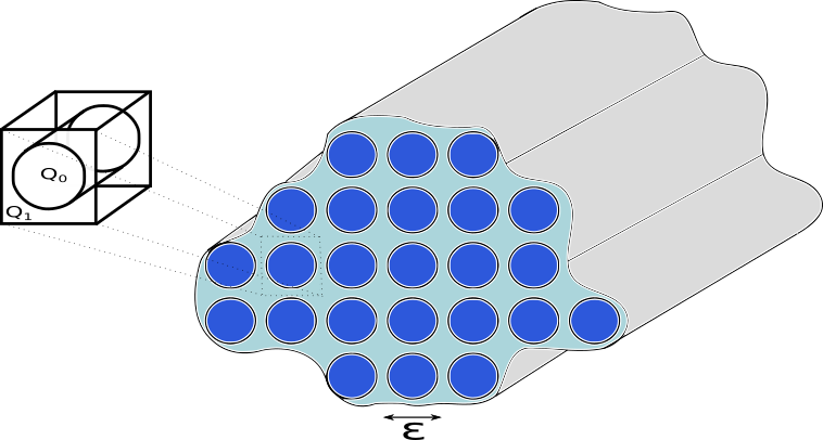 Figure 1
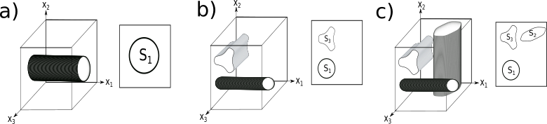 Figure 2
Peer Reviews
No public reviews on file for this paper yet. If you reviewed it on a platform where reviews are public (OpenReview, ICLR, NeurIPS, ICML), you can paste yours below so the community can read it here.
Videos
No videos yet. Explain this paper in a talk, walkthrough, or lecture? Add one.
Taxonomy
TopicsAdvanced Mathematical Modeling in Engineering · Composite Material Mechanics · Numerical methods in inverse problems
Quasi-periodic two-scale homogenisation and effective spatial dispersion in high-contrast media
Shane Cooper
Abstract
The convergence of spectra via two-scale convergence for double-porosity models is well known. A crucial assumption in these works is that the stiff component of the body forms a connected set. We show that under a relaxation of this assumption the (periodic) two-scale limit of the operator is insufficient to capture the full asymptotic spectral properties of high-contrast periodic media. Asymptotically, waves of all periods (or quasi-momenta) are shown to persist and an appropriate extension of the notion of two-scale convergence is introduced. As a result, homogenised limit equations with none trivially quasi-momentum dependence are found as resolvent limits of the original operator family. This results in asymptotic spectral behaviour with a rich dependence on quasimomenta.
1 Introduction
The model problem to study time-harmonic waves, with frequency , in media with microstructure is
[TABLE]
where the wave represents the information being propagated, such as pressure in acoustics, deformation in elasticity or electromagnetic fields in electromagnetism111In elasticity and electromagnetism the wave equation describes certain polarised waves: e.g. Shear polarised wave in elasticity or Transverse Electric and Transverse Magnetic polarised waves for the Maxwell system.. The microstructured nature of the media is characterised by periodic coefficients a_{\varepsilon}\222The implied non-trivial dependence of on is deliberate and, as we shall see, important. :
[TABLE]
where , are (the square-root of) the wave speeds of the individual constitutive material components, see figure 1.
The parameter represents the ratio between the size of the microstructure and the observable length scale, and is typically taken to be small. From the point of view of applications, it is important to study the asymptotic behaviour of these waves in the limit of vanishing .
A classical approximation, provided by the homogenisation theorem333Also called the long-wavelength or quasi-static approximation depending on the community., states that for fixed frequency the microstructured media can be approximated by an ‘effective’ homogeneous media whose wave speed is constant and determined directly from the ‘local periodic’ behaviour of the problem. The intuition behind why the homogenisation theorem holds is that the ‘wavelength’ of is long with respect to the microstructure: variations in appear over much longer distances than the media’s period. Mathematically, this is ensured by assuming that are taken to be uniformly bounded and elliptic with respect to , for example
[TABLE]
It has been known for some time now that interesting effects appear when the above elliptic conditions are not uniform. This happens for example in so-called high-contrast media. In the context of waves, high-contrast media of particular interest are the so-called double porosity models which admit the ‘critical’ scaling:
[TABLE]
Physically, this critical scaling corresponds to the wavelength of remaining ‘long’ within the media but in media the wavelength is at the ‘resonant’ scale, i.e. of the same order as the size of the microstructure. Thus violating the underlying intuition for the long-wavelength approximation.
The mathematical analysis of high-contrast problems has given rise to rigorous descriptions of various scale-interaction phenomena such as memory effects and other non-local effects (e.g. [17, 28, 5, 7, 8, 9, 14]). Within the context of wave propagation, an important feature of high-contrast problems is that they contain spectral gaps (cf. [18, 30, 31]): frequencies at which no wave can propagate through the underlying medium. Such gaps are important from the point of view of wave-guiding applications such as photonic crystal fibres.
An important initial work in the study of the spectrum of high-contrast elliptic operators was undertaken by V. V. Zhikov [30, 31]. Therein, the homogenisation theory for double porosity-type problems was developed within the framework of the so-called two-scale convergence of G. Nguetseng-G. Allaire [27, 1]. Using this theory, Zhikov derived two-scale limit spectral equations that contain a non-trivial coupling between micro- and macro-scales. Such a coupling leads to an eigenvalue problem with a highly non-linear spectral dependence, described by a function . The convergence of spectra (in the appropriate sense) was proved and, by doing so, demonstrates that this function provides an explicit description of the asymptotic structure of the spectrum. Such an explicit description of the limit spectral behaviour via two-scale homogenisation has made way for mathematical studies of high-contrast media as wave-guides: in [20] using multi-scale asymptotics and supplemented with analysis based on two-scale convergence in [10].
Moreover, the Zhikov function was later independently discovered by G. Bouchitté and D. Felbacq [6] in the specific context of TM-polarised electromagnetic wave propagation in a dilute dielectric two-dimensional photonic crystal fibre; therein the authors made the interesting interpretation of the -function playing the role of effective negative magnetism. Later, in the context of elasticity, a matrix analogue of the function is derived and plays the role of frequency-dependent effective density [3, 4, 32]. Such works demonstrate that the unusual phenomena observed in high-contrast media can be described by non-standard constitutive laws provided via two-scale homogenisation.
The idea that high-contrast media can result in the appearance of non-standard constitutive laws and give rise to composite media with complex wave phenomena near micro-resonances has prompted a recent energetic pursuit of such laws in the contexts of elasticity (e.g. [24]) and electromagnetism (e.g. [22, 12]). Applications can be found in areas such as cloaking (e.g. [25, 26]). It was shown in the work of V. P. Smyshlyaev [29], building on related ideas in [14], that the two-scale homogenised limit of various anisotropic elastic media contain not only the temporal non-locality (as described by the Zhikov function) but also exhibit spatial non-locality. The presence of which leads to the phenomena of ‘directional’ localisation: the number of admissible propagating wave modes depends not only on the frequency but on the direction of propagation. Such a feature is important for cloaking applications. These motivating works have led to recent systematic study containing rigorous asymptotic and spectral analysis of general mathematical constructions containing ‘high-contrasts’ [21]. Analysis based on the work [21] has led to the demonstration that the two-scale convergence is insufficient to fully study the spectrum of general high-contrast problems, see [15, Chapter 5],[11]. The reason for this inconsistency is due to the presence of quasi-periodic micro-oscillations that persist at leading-order in general high-contrast media.
In this work we appropriately develop homogenisation theory to study quasi-periodic micro-oscillations. This is achieved by extending the two-scale convergence framework to admit such oscillations. We explain the (lack of the) role these micro-oscillations in the numerous previous works on high-contrast problems. Then, we apply this theory in the spectral analysis of a novel class of high-contrast media. In particular, we shall show that by relaxing the geometric assumptions in the double-porosity model leads to multi-scale homogenised models that contain a new feature: the effective wave speed depends on the quasi-momenta in a highly discontinuous fashion. Specifically, the non-standard constitutive equations for such high-contrast media exhibit spatial dispersion. The presence of this novel feature is related to the contribution of the quasi-periodic waves on the microscale.
Notations
We end the introduction with some words on the notation used in this article.
Vectors and vector-valued functions are represented by lower-case boldface symbols with the exception of the co-ordinate points. denotes the Euclidean basis in . For a vector , we denote by its component with respect to , and write
[TABLE]
Points in will be denoted by the symbol and points in the unit cell will be denoted by . The notation will be used to denote partial differentiation with respect to the -th coordinate variable, and we shall replace the suffix with or when we wish to emphasis the macroscopic or microscopic variable. Similarly, the notion , , , and , are used for the divergence or gradient of a function in terms of or .
Throughout is a domain in , , and . All of the functions, even if real-valued, are considered to take values in the complex field.
The space denotes the usual space of smooth -periodic functions. Whereas, shall denote the space of smooth functions whose functions and derivatives are -quasi-periodic with respect to : for each and each Euclidean basis vector , . Equivalently,
[TABLE]
Note that and use the latter to avoid confusion with the notation for the space compactly supported smooth functions.
The Sobolev space is the usual Sobolev space of -periodic functions. Whereas is defined as the closure of with respect to the norm, or equivalently as
[TABLE]
Also, we note and, in this situation, we use the latter to avoid confusion with the Sobolev space of zero trace functions.
For subsets and of we say that converges to in the Hausdorff sense if the following conditions hold:
For every such that converges to some , then . 2. 2.
For every there exists such that .
We shall use the notation when a sequence of sets Hausdorff converges to .
The Einstein summation convention will not be used in this article, that is we do not sum with respect to repeated indices.
2 Quasi-periodic two-scale convergence
In this section we introduce an appropriate notion of convergence that will account for the presence of microscopic oscillations that are quasi-periodic in nature. This convergence will turn out to be a natural extension of the standard (periodic) two-scale convergence introduced by G. Nguetseng[27]-G. Allaire [1]. In particular, we aim to use this extended notion of two-scale convergence to study the spectral properties of operator families in homogenisation theory in a similar vein to that first introduced by V. V. Zhikov [30, 31].
2.1 Motivation
We shall motivate the notion of quasi-periodic two-scale convergence here. This motivation is based on the principle goal of characterising the spectral asymptotics of high-contrast elliptic operators.
Let be a sequence of positive real numbers with limit zero. Consider the differential operator whose action is given by
[TABLE]
and domain consists of for which . Here are -periodic measurable functions, that are bounded and elliptic: such that
[TABLE]
In this article, we focus on that are uniformly bounded, i.e. is independent of , but may degenerate in the sense that with . We are interested in analysing the structure of the spectrum of in the limit of . The strategy of the study is to establish the existence of some operator such that Hausdorff converges to ; i.e. the following conditions hold:
For every such that converges to some we deduce that . 2. 2.
For every we find such that .
A crucial question is how to determine the operator . For example, in classical and semi-classical high-contrast problems, turns out the be the strong two-scale resolvent homogenised limit of , cf. [30, 31, 16]. To develop some intuition on what to expect in the general case, let us recall an important result from the spectral theory of elliptic operators with -periodic coefficients: the Floquet-Bloch decomposition (see for example [23] for more details). This result states that the following characterisation of holds:
[TABLE]
where , describe a family of densely defined self-adjoint operators with compact resolvent given by the action that if solves
[TABLE]
Taking the above into consideration we see that if, and only if, there exists and non-trivial such that
[TABLE]
By a change of variables and , we see that solves
[TABLE]
and belongs to the space of functions that satisfy the condition
[TABLE]
for some . This condition is typically referred to as the Bloch or quasi-periodic condition and is known as the quasi-momentum. Note that is the usual periodicity condition. The Sobolev space of -quasi-periodic functions coincides with which, we recall, is be defined as
[TABLE]
The general principle to observe here is that if we wish to study the asymptotic behaviour of the spectrum we need to keep track of the eigenfunctions that are -quasi-periodic on micro-scale , for all . The notion of quasi-periodic two-scale convergence, introduced in Section 2.2 below, performs such a task.
We note here that in the case of the whole space, as discussed above, one need not refer to a notion of quasi-periodic two-scale convergence to study the asymptotics of the spectrum; one may study the norm-resolvent limits of the operators to study spectral asymptotics, cf. [18] where the point-wise (in ) limits or [13] where the uniform limits were considered in the double-porosity setting. That being said, for boundary-value problems, the Bloch decomposition does not hold; nevertheless, the whole space (or Bloch) spectrum is expected to contribute asymptotically to the bounded domain spectrum and the precluding discussion is still relevant. It is this setting that the quasi-periodic two-scale convergence will be particularly useful.
Finally, we comment that the above discussion leads to the natural question: why in previous cases considered was it sufficient to consider the standard (periodic) two-scale limit of to ensure spectral convergence? Or put another way, when in the asymptotic limit of do we need consider all quasi-periodicity and not just . This shall be explained in Section 2.3.
2.2 Definition and basic properties
This section is dedicated to the introduction of the notion quasi-periodic two-scale convergence and an exposition of results that are appropriate to homogenisation theory.
Recall denotes the usual space of smooth -periodic functions and
[TABLE]
The following mean-value property will be important: For every and every the following convergence
[TABLE]
holds. This fact follows by noting that the assertion holds for elements in , see for example [1, Lemma 1.3], and observing that multiplication by defines an isomorphism between and that preserves absolute value. Indeed, belongs to if, and only if, belongs to and in .
We remark here that because is isomorphic to , with isomorphism {\rm exp}\big{(}-\rm i{\boldsymbol{\theta}}\cdot y\big{)}, then the results presented in this section444The results in this section can be established by first principles making no reference to such an isomorphism. are immediately established for each if proved for . We shall demonstrate this with the first result of the section and omit the remaining proofs which follow in a similar manner.
Definition 1**.**
Let be a bounded sequence and . Then, we say (weakly) -quasi-periodic two-scale converges to , denoted by , if the following convergence
[TABLE]
holds.
Remark 1*.*
Notice that for , this is the standard notion of two-scale convergence.
The next important result states that bounded sequences in are relatively compact with respect to quasi-periodic two-scale convergence.
Proposition 1**.**
If is bounded in then, up to a subsequence, weakly -quasi-periodic two-scale converges to some .
Proof.
The result has been established previously for the case , see for example [27, 1, 30]. Let us consider . Note that the function \widetilde{u}_{\varepsilon}={\rm exp}\big{(}-\rm i{\boldsymbol{\theta}}\cdot y\big{)}u_{\varepsilon} is bounded in and therefore by the assertion for , up to a discarded subsequence, (-quasi-periodically) two-scale converges to some . Now, the result follows from this fact and noting that for fixed one has
[TABLE]
and that {\rm exp}\big{(}-\rm i{\boldsymbol{\theta}}\cdot y\big{)} is a smooth periodic function. Hence u_{\varepsilon}\overset{2-{{\boldsymbol{\theta}}}}{\rightharpoonup}{\rm exp}\big{(}\rm i{\boldsymbol{\theta}}\cdot y\big{)}\widetilde{u}. ∎
An important result from the point of view of homogenisation theory is that the test functions in (2.3) can be taken to be quasi-periodic elements of , i.e. the following result holds.
Proposition 2**.**
If -quasi-periodic two-scale converges to , then the following convergence
[TABLE]
holds for all , and for all such that for almost every and .
Remark 2*.*
If is a bounded domain, as in this article, then additionally the test functions can be taken to be elements of .
The following results are of interest.
Proposition 3**.**
For -quasi-periodic two-scale converging to one has that
[TABLE] 2. 2.
For -quasi-periodic two-scale converging to then
[TABLE]
A result of particular interest in high-contrast homogenisation problems is the following.
Proposition 4**.**
Let satisfy
[TABLE]
Then, there exists such that, up to a subsequence, the following convergences hold:
[TABLE]
Recall here that is given by (1.1).
Proof.
Let and denote respectively fixed arbitrary elements of and . By Proposition 1, there exists and such that, up to a discarded subsequence, the following convergences hold:
[TABLE]
Note that, since is bounded in , then strongly converges to zero in and from Proposition 3 part 2. we conclude that
[TABLE]
Let us prove that . Using the convergences (2.4) and (2.5) we pass to the limit in the identity
[TABLE]
to deduce that
[TABLE]
Therefore, for almost every , the functions and are related by the identity
[TABLE]
It is clear that C^{\infty}_{0}\big{(}(0,1)^{d}\big{)}\subset C^{\infty}_{{\boldsymbol{\theta}}}(\square) and so with . It remains to show belongs to . This follows from noting that after performing integration by parts in the above identity we arrive at
[TABLE]
Setting above, for arbitrary smooth -periodic , demonstrates that is an element of that satisfies periodic boundary conditions with respect to . That is, and so (see definition (1.1)) . ∎
We end this section with a result that is illuminating when it comes to studying the convergence of spectra for parameter-dependent operator families. It readily provides a one-sided justification for the Hausdorff convergence of the high-contrast spectra to the spectrum associated to quasi-periodic two-scale limits. This result is based on the following definition, which extends the notion of strong resolvent two-scale convergence first introduced by V. V. Zhikov in [30, 31].
Definition 2**.**
Fix , and let and be non-negative self-adjoint operators respectively defined in and a closed subset of . We say that strong resolvent -quasi-periodic two-scale converges to if for every that -quasi-periodic two-scale converges to , the following convergence
[TABLE]
holds. Here, is the orthogonal projection onto in .
Here, we state an important consequence of such resolvent convergence. The proof, omitted here, follows standard spectral theoretic arguments, see for example [30].
Proposition 5**.**
If strong resolvent -quasi-periodic two-scale converges to then the spectrum of is related to the spectrum of in the following sense:
For every there exists such that converges to as tends to zero.
2.3 On the relevance of quasi-periodic two-scale convergence in spectral asymptotics
Proposition 5 informs us that, in principle, one should consider all strong quasi-periodic two-scale limits of an operator to fully characterise its limit spectrum (in the Hausdorff sense). Yet, clearly this is not always the case: such a notion of convergence has not appeared previously, nor was it needed, to study the spectral asymptotics of classical and particular double-porosity operators. The reason for this shall be elucidated here. Moreover, at the end of this section we shall argue when quasi-periodic convergence is necessary via a model problem that we later study in detail in this article.
2.3.1 Classical homogenisation
Consider the resolvent problem: For fixed find such that
[TABLE]
where the symmetric matrix-valued function is -periodic, elliptic and bounded: such that
[TABLE]
The following homogenisation theorem is classical.
Theorem 1** (Classical homogenisation theorem).**
Let be a sequence with limit [math], and a sequence such that weakly converges in to some as tends to zero. Then the solution to (2.6), for , converges weakly in (and strongly in ) to the solution to
[TABLE]
Here is the constant symmetric homogenised matrix determined by :
[TABLE]
It is well-known that the homogenisation theorem implies the Hausdorff convergence of spectra (cf. [2, Section 2]):
[TABLE]
Let us study the quasi-periodic two-scale limits of .
Proposition 6**.**
Fix and consider such that . Then, -quasi-periodic two-scale converges to zero; that is .
Remark 3*.*
Proposition 6 informs us that for the classical resolvent problem (2.6), the non-zero quasi-periodic micro-oscillations at leading order do not contribute to the spectral asymptotics. So one need only study the quasi-periodic oscillations, i.e. the standard two-scale limit. It is well-known that the (periodic) two-scale limit coincides with the classical limit provided by Theorem 1, see for example [1, 30]. 2. 2.
The part of the spectrum corresponding the -quasi-periodic micro-oscillations, for , actually resides in an neighbourhood of infinity; this can be formally seen from the considerations of Section 2.1: for independent of , the eigenvalues in (2.1) are clearly of the order . To study such ‘high-frequency’ spectrum one can consider the re-scaled operator , that is consider coefficients of the form . The precise study of such high-frequency spectra was performed in [2] for a broader class of moderately contrasting locally periodic coefficients. Therein, the authors provide a rigorous description of the high-frequency spectral asymptotics in terms of non-trivial quasi-momenta . This was done by introducing an appropriate notion of “Bloch wave homogenisation”. For the reduced setting of (globally) periodic coefficients, the Bloch-wave operator-limits determined therin can readily be shown to be equivalent to the -quasi-periodic two-scale limits.
Proof of Proposition 6.
The sequence weakly converges, cf. Proposition 3 part 1., and so is bounded. Multiplying (2.6) (for ) and integrating over , and using the ellipticity of , produces the a-priori bound
[TABLE]
Applying Proposition 4, we deduce that there exists such that, up to a subsequence, the following convergences hold:
[TABLE]
Let us show : is a bounded sequence and so strongly converges to zero in . Therefore, by Proposition 3 part 2., we deduce . As is connected it follows that is constant. Yet and there are no non-trivial constant -quasi-periodic functions for , see (1.1). Hence, . ∎
2.3.2 Double-porosity model
Consider the resolvent problem: For fixed find such that
[TABLE]
Here
[TABLE]
where is a smooth compactly contained subset of such that, for , the periodic extension
[TABLE]
forms a connected set in . The functions , are taken to be real-valued, elliptic and bounded on . The following homogenisation theorem is established in [30, Theorem 5.1].
Theorem 2**.**
Suppose in the right-hand side of (2.7) two-scale converges to some , that is for . Then, the sequence of solutions two-scale converges to , where belongs to
[TABLE]
and uniquely solves
[TABLE]
Here, is the constant symmetric and positive homogenised matrix for perforated domains determined by :
[TABLE]
This result informs us that strongly two-scale converges to the operator , defined in , associated to the above two-scale limit resolvent problem. Therefore, by Proposition 5 for , the lower-semicontinuity of the spectral convergence is ensured. In fact, Zhikov proved in [30, Theorem 8.1], under the condition that is connected in , the stronger result
[TABLE]
Let us determine the strong resolvent quasi-periodic two-scale limits of .
Proposition 7**.**
Fix . Suppose in the right-hand side of (2.7) such that to some . Then, the sequence of solutions -quasi-periodically two-scale converges to the solution to
[TABLE]
Remark 4*.*
-
Note that is independent of for , and its spectrum is the point spectrum given by the operator whose action is with domain .
-
It is easy to see (by noting that setting in (2.8) gives (2.9)) and so
[TABLE]
The set
[TABLE]
is the limit spectrum arriving from quasi-periodic micro-oscillations.
The restriction of the limit spectrum to is achieved by considering the purely macro-scopic component (of eigenfunctions) to be zero. For this reason, we coin this spectrum to be pure Bloch spectrum. In the simplified setting of double-porosity the pure Bloch spectrum is point spectrum (due to the fact is independent of for ). In general, we expect this spectrum to have band-gap structure, and the gaps have only contracted to points here due to the geometric constraint that is connected in . This expectation is verified in Section 6.
- Even though the strong resolvent -quasi-periodic limit of exists, it has trivial dependence on , and more importantly is a restriction of the two-scale limit . Hence, one need only consider , and this explains why in this setting one is to expect Zhikov’s result . In general, the limit will not be sufficient to capture the full spectral asymptotics.
Proof of Proposition 7.
Let us consider (respect. ) to be extended by zero into (respect ), and consider to be the constant such that
[TABLE]
The solution solves
[TABLE]
Setting in the above variational problem and using the fact that , we deduce the a-priori bound (for )
[TABLE]
Additionally, we have the bound
[TABLE]
Indeed, and
[TABLE]
By Proposition 4 it follows that, up to a discarded subsequence,
[TABLE]
for some .
Let us show that . By Proposition 2 it follows that
[TABLE]
Yet strongly converges to zero in . Therefore , which is equivalent to on (recall is positive on and zero on ). As is connected then is constant in . Now, since the periodic extension forms a connected set then is constant in . Yet, for and consequently this constant is zero, cf (1.1).
It remains to prove solves (2.9). This can easily be deduced by passing the the -quasi-periodic limit in (2.10) for test functions , , and using convergences (2.11). ∎
2.3.3 An example with non-trivial quasi-periodic limits
Let us provide an example which demonstrates that in general the family , of strong resolvent -quasi-periodic limits to , are not restrictions of .
Suppose, we consider (2.7) for coefficients
[TABLE]
and are real-valued -functions such that and . Let be a bounded sequence and solve (2.7) for . Arguing as in the proof of Proposition 7, we see that to solution to (2.7) will satisfy the a-priori bounds
[TABLE]
In particular, Proposition 4 informs us that up to a subsequence
[TABLE]
for some . Moreover, by an application of Proposition 2 we deduce that
[TABLE]
Denoting by the closed linear subspace of given by555The space was first introduced in [29] and coined the space of microscopic oscillations. We have appropriately extended this notion to -quasi-periodic oscillations here, .
[TABLE]
Suppose we show an example where is not a subset of for some non-trivial , . Then, for such examples we should not expect that is an extension of , nor should we expect . Let us provide such an example. The conjectures (stated immediately above) based on this example will be proved rigorously in the remainder of the article.
Suppose is the cylinderical domain
[TABLE]
and
[TABLE]
Notice that the periodic extension of into consists of infinitely many mutually disjoint cylinders , . That is, the assumptions of Subsection 2.3.2, and in particular [30, 31], do not hold.
Now if, and only if, with for some on . This implies, cf (1.1), that
[TABLE]
(in the sense of trace). Then, for we arrive at the condition
[TABLE]
Therefore, if , then the above condition only holds if . That is must necessarily be zero on . On the other hand, if then any function that is constant on belongs to . In particular we see that does not belong to for all .
Remark 5*.*
Note that if contains a connected subset which joins two opposite faces of the square then the space non-trivially depends on . Consequently, non-trivial limit Bloch spectrum is expected for aligned orthogonally to these faces.
The remainder of the article is dedicated to determining the strong quasi-periodic two-scale limits of for such fibre-like inclusions. Moreover, we demonstrate that indeed are not restrictions of and that form non-trivial subsets of .
3 Problem formulation and Homogenisation
In this article we are concerned with the asymptotic analysis of the resolvent problem
[TABLE]
where is a small parameter, is a smooth open bounded star-shaped domain666All the results and proofs follow through in an identical manner for the case where is the whole space. and known. The coefficient is given by
[TABLE]
and the regions and are described as follows (cf. Figure 2).
Geometric assumptions. For we consider smooth domains compactly contained in that have mutually disjoint closures. We denote by the cylinder aligned to the -th co-ordinate axis with cross-section , i.e. C_{1}:=\{y\in(0,1)^{3}\,\big{|}\,y\in(0,1)\times S_{1}\}, C_{2}:=\{y\in(0,1)^{3}\,\big{|}\,y=(z_{2},z_{3},z_{1}),z\in(0,1)\times S_{2}\} and C_{3}:=\{y\in(0,1)^{3}\,\big{|}\,y=(z_{3},z_{1},z_{2}),z\in(0,1)\times S_{3}\}.
Then, for a given non-empty subset of , we consider . We denote by and .
Under this geometric assumption we determine for each the strong resolvent -quasi-periodic two-scale limit, cf. Section 2, of the self-adjoint operator associated to resolvent problem (3.1). That is, for a fixed and a given bounded sequence such that , i.e.
[TABLE]
we aim to determine the -quasi-periodic two-scale limit behaviour of the solution to
[TABLE]
As is bounded in , upon setting in (3.3) we deduce that the sequences
[TABLE]
are bounded. Let us describe the -quasi-periodic two-scale limit, referring to Section 4 for the details.
The limit of will be a function , of two variables , , that is -quasi-periodic with respect to the second variable , cf Proposition 4. Furthermore, due to the fact that in each cylinder , , the gradient of is bounded, the limit necessarily belongs to the (Bochner) space where
[TABLE]
It follows from this (see (1.1)) that is non-zero in cylinder if and only if the -th component of is zero. If , then we determine that is not only non-trivial but it is actually more regular in the -th coordinate direction: .
More precisely, for the subset of indexes given by , we denote by the closed subspace of spanned by ,777Note that is either the whole space, a plane or a line in . and show that the function belongs to the set
[TABLE]
which is clearly a Hilbert space when endowed with the inner product
[TABLE]
Here, is the outer unit normal to .
For each fibre there corresponds an effective constant material parameter given by
[TABLE]
where N^{(i)}\in H^{1}_{\#_{i}}(C_{i}):=\{u\in H^{1}(C_{i})\,|\,u\text{ is 1y_{i}}\} is the unique solution to the cell problem
[TABLE]
Then, for each , the -quasi-periodic two-scale limit problem is formulated as follows: For find such that
[TABLE]
As are positive numbers and it follows that the left-hand side of the above problem defines an equivalent inner product on the space , and consequently the existence and uniqueness of solutions to (3.9) are ensured by the Riesz representation theorem.
Setting on in (3.9) gives the equation
[TABLE]
and a subsequent integration by parts in (3.9) leads to the variational formula
[TABLE]
for all , such that . For each fixed we set , and for , above. This leads to the -quasi-periodic two-scale homogenised system of equations.
[TABLE]
Here
[TABLE]
for the outer unit normal of . We now state the main result of the article.
Theorem 3**.**
Consider , such that , and the solution to (3.3). Then converges, up to some subsequence, in the -quasi-periodic sense to the unique solution to (3.9), equivalently (3.10).
An immediate consequence of Theorem 3 is that for each , the operator strong resolvent -quasi-periodically two-scale converges to the operator associated to problem (3.10), see Definition 2 in Section 2. Consequently, Proposition 5 informs us that the lower semi-continuity of the spectra in the Hausdorff sense is ensured:
[TABLE]
The structure of the limit spectrum is analysed in Section 6 and described in Proposition 10.
Remark 6*.*
A seperate issue, not explored here, is the so-called spectral completeness statement, i.e. the question of whether or not the remaining criterion for Hausdorff convergence of spectra is satisfied: does it follow that
[TABLE]
In general this will not be true due to the presence of the boundary, and the fact that intersects the boundary. This leads to the expectation that there exists non-trivial spectrum due to surface waves asymptotically localised near the boundary, cf. [2] for analoguous results in the context of classical locally periodic media. For the case of being the torus or the whole space the above assertion is expected to hold and will be explored in future works.
4 Proof of the homogenisation theorem
This section is dedicated to the proof of Theorem 3. To do this, we shall develop an appropriate quasi-periodic two-scale variation of a powerful method first introduced in [21] in the context of standard (periodic) two-scale convergence, i.e. -quasi-periodic two-scale convergence for . In what follows , and will denote respectively fixed arbitrary elements of , and .
4.1 Technical preliminaries
The following results will be of importance in the proof of the homogenisation theorem.
Lemma 1**.**
Let be the closure of a smooth domain and let be a smooth bounded domain such that and is a connected set. Then every u\in H^{1}\big{(}(0,1)\times A\big{)} can be extended to as a function \widetilde{u}\in H^{1}\big{(}(0,1)\times B_{1}\big{)} such that
[TABLE]
where does not depend on .
Proof.
Suppose u\in H^{1}\big{(}(0,1)\times A\big{)}. Then, by Fubini’s theorem, for almost every the function belongs to and let be the Sobolev extension of into given in [19, Lemma 3.2, pg. 88]. In particular, one has
[TABLE]
where does not depend on nor . Here, denotes the gradient vector .
Consider given by
[TABLE]
Then and from assertion (4.2) it follows that
[TABLE]
To prove (4.1), it remains to demonstrate that \partial_{x_{1}}\widetilde{u}\in L^{2}\big{(}(0,1)\times B_{1}\big{)} and
[TABLE]
For each , the difference quotient is given by
[TABLE]
where we have extended trivially by zero into . Notice that , i.e. the extension into of the function , and consequently
[TABLE]
Since converges strongly in L^{2}\big{(}(0,1)\times A\big{)} to , it follows that is a Cauchy sequence in L^{2}\big{(}(0,1)\times B_{1}\big{)} and this limit can be identified, using the fact that for \phi\in C^{\infty}_{0}\big{(}(0,1)\times B_{1}\big{)}, as . Furthermore, passing to the limit in the above inequality yields (4.4). ∎
Proposition 8**.**
Fix . There exists a constant such that
[TABLE]
Here V_{{\boldsymbol{\theta}}}={\rm ker}\sqrt{a_{1}}\boldsymbol{\nabla}_{{\boldsymbol{\theta}}}=\{u\in H^{1}_{{\boldsymbol{\theta}}}(Q)\,\big{|}\,\sqrt{a_{1}}\boldsymbol{\nabla}u\equiv 0\}.
Proof.
For each , let be the cross-section of the cylinder . Since are compactly contained in and have mutually disjoint closures then there exists open such that and are mutually disjoint. Let be smooth cut-off functions that are identity on , we extend by zero to .
Now using Lemma 1, let be the extension of to , where is the cylinder whose axis is parallel to with cross-section . Note that since is -quasi-periodic in the variable , then the extension will be also, see (4.3). By Lemma 1 it follows that
[TABLE]
For , the following Poincaré inequality
[TABLE]
holds888This follows from noting the lower bound on the spectrum of the laplacian on the space of functions that are -quasi-periodic in direction .. For , one has
[TABLE]
for some . Here .
Recalling, , we set , here are taken to be constant in the variable and as above the complementary directions. It follows that and . Note that, by construction and inequalities (4.6), and (4.7), one has
[TABLE]
Now, the positivity of on and (4.5) imply that the element of is such that
[TABLE]
and the result follows.
∎
4.2 Proof of Theorem 3
Consider the sequence of solutions to (3.3), i.e.
[TABLE]
for , and recall, cf. (3.4), that
[TABLE]
Consequently, Proposition 4 informs us that a subsequence of -quasi-periodic two-scale converges to some , and moreover . Let us study the structure of this limit further.
We begin by introducing the densely defined unbounded linear operator which is given by the action
[TABLE]
We now argue that a generalised Weyl’s decomposition holds, which was first introduced and proved for the case in [21].
Lemma 2**.**
Let denote the adjoint of . Then, the orthogonal decomposition
[TABLE]
holds.
Remark 7*.*
Lemma 2 is a generalisation of the well-known fact that (periodic) divergence-free vector fields are mutually orthogonal to gradients of (periodic) potentials in . In fact, this classical result can be deduced from the above lemma by (formally)999In fact, as expected the proof of this statement for is much easier as is positive where as is non-negative. setting on .
Proof of Lemma 2.
By the Banach closed ranged theorem, this result will follow if we demonstrate that the range of is closed, and this fact is implied by Proposition 8.
Indeed, suppose converges strongly in to some as , i.e. there exists such that converges strongly in to . By Proposition 8, the sequence , where denotes the orthogonal projection of onto the orthogonal complement of in , is a Cauchy sequence in and therefore converges, up to some subsequence, to . In particular, converges strongly in to and, consequently . Hence, the range of is closed. ∎
Let us now describe in detail.
Lemma 3**.**
*The function belongs to the Bochner space . *
Proof.
Recall that
[TABLE]
and so we aim to show that .
On the one hand we deduce from (4.9) and (2.2) that
[TABLE]
Yet, on the other hand, Proposition 2 and the assertion imply
[TABLE]
Therefore, as finite sums of are dense in it follows that and since we find that . ∎
The following result is of fundamental importance in characterising the (-quasi-periodic) limit of the flux in terms of the limit of the function . Put another way, this identity is crucial for determining the homogenised coefficients.
Lemma 4**.**
There exists such that, up to a subsequence, . Moreover, belongs to the Bochner space L^{2}\big{(}\Omega;{\rm ker}\big{(}(\sqrt{a_{1}}\boldsymbol{\nabla}_{{\boldsymbol{\theta}}})^{*}\big{)}\big{)} and the pair satisfies the identity
[TABLE]
Proof.
By Proposition 1 and (4.9) there exists such that, up to a subsequence that we discard, one has
[TABLE]
To prove \boldsymbol{\xi}\in L^{2}\big{(}\Omega;{\rm ker}\big{(}(\sqrt{a_{1}}\boldsymbol{\nabla}_{{\boldsymbol{\theta}}})^{*}\big{)}, we take in (4.8) test functions of the form , , , and use (4.9), (4.11) to pass to the limit in and deduce that
[TABLE]
Therefore, for almost every one has
[TABLE]
and, hence by Lemma 2 it follows that \boldsymbol{\xi}(x,y)\in L^{2}\big{(}\Omega;{\rm ker}\big{(}(\sqrt{a_{1}}\boldsymbol{\nabla}_{{\boldsymbol{\theta}}})^{*}\big{)}.
Let us now prove assertion (4.10). Henceforth, we consider \Psi\in{\rm ker}\big{(}(\sqrt{a_{1}}\boldsymbol{\nabla}_{{\boldsymbol{\theta}}})^{*}\big{)} to be -quasi-periodically extended to . We shall prove below the following “integration by parts” formula:
[TABLE]
Using Proposition 2, (4.11) and the convergence , we pass to the limit in the above formula to readily arrive at (4.10).
To prove (4.12), it is sufficient to prove the following: for every one has
[TABLE]
Indeed, (4.12) follows from utilising (4.13) and the following facts: for then belongs to , as , and can be trivially extended to , and that
[TABLE]
Let us now prove (4.13). For , , it follows that
[TABLE]
where the last equality comes from the change of variables and recalling that is periodic and is -quasi-periodic. By noting, for , that
[TABLE]
is an element of , and that
[TABLE]
the identity (4.13) follows. ∎
We are now ready to describe the properties of the macroscopic part of and express the flux in terms of .
Lemma 5**.**
Let , and \boldsymbol{\xi}\in L^{2}(\Omega;{\rm ker}\big{(}(\sqrt{a_{1}}\boldsymbol{\nabla}_{\boldsymbol{\theta}})^{*}\big{)}, be a pair which satisfies the identity (4.10). Then, , see (3.6). That is, for every for , one has on , where with on , for the outer unit normal to . Furthermore,
[TABLE]
Here, solve (3.8).
The following result immediately follows from the above lemma.
Proposition 9**.**
For every for , one has
[TABLE]
Here, are given by (3.7), i.e.
[TABLE]
for N^{(i)}\in H^{1}_{\#_{i}}(C_{i})=\{u\in H^{1}(C_{i})\,|\,u\text{ is 1y_{i}}\} is the unique solution to the cell problem
[TABLE]
Proof.
Equation (4.14) implies
[TABLE]
For each , we set in (4.15) to determine that
[TABLE]
Hence, it follows that
[TABLE]
for almost every . Finally, from (4.15) it follows that
[TABLE]
Then, the positivity of can be seen by the inequality
[TABLE]
and noting that the right-hand side of this inequality can not be zero for this would contradict the periodicity of in the variable. ∎
Proof of Lemma 5.
As , see Lemma 3, then is constant in each fibre , . Now if then is necessarily zero in . On the other hand, if , i.e. , then for , . That is, on for some , where we recall that is the closed subspace of spanned by .
Let us now demonstrate that belongs to the Hilbert space By substituting on , , into (4.10), we deduce that
[TABLE]
For fixed , we will show directly below that there exists a function \boldsymbol{\Psi}^{(j)}{\ker}\big{(}(\sqrt{a_{1}}\boldsymbol{\nabla}_{\boldsymbol{\theta}})^{*}\big{)} such that
[TABLE]
Therefore
[TABLE]
and consequently substituting into (4.16) gives
[TABLE]
That is, and on where is the outer unit normal to , i.e. if (4.17) holds.
To show (4.17), we note that under the geometric assumptions on cylinders , , there exists a function
[TABLE]
Then, for each , the function clearly satisfies (4.17). Furthermore, belongs to {\ker}\big{(}(\sqrt{a_{1}}\boldsymbol{\nabla})^{*}\big{)}: Indeed, as , an element is -periodic in the variable , and it follows
[TABLE]
Therefore, (4.17) holds.
Let us now demonstrate (4.14). For , and almost every , notice that
[TABLE]
and, by the geometric assumption of the cylinders, we can extend into such that the extensions are elements of and equal to zero on . Therefore, it follows that
[TABLE]
Consequently, (4.16) takes the form
[TABLE]
Integrating by parts above, which is permissible since , we deduce that
[TABLE]
That is, for almost every , is the projection onto \ker\big{(}(\sqrt{a_{1}}\boldsymbol{\nabla}_{{\boldsymbol{\theta}}})^{*}\big{)} of the function
[TABLE]
For each , let given by (4.18), and we introduce the extension into , given by Lemma 1, of the function that solves (4.15). It follows that belongs to and
[TABLE]
for all . That is, belongs to \ker\big{(}(\sqrt{a_{1}}\boldsymbol{\nabla}_{{\boldsymbol{\theta}}})^{*}\big{)}. Obviously
[TABLE]
and
[TABLE]
since is piece-wise constant on . Consequently, as is the projection of onto \ker\big{(}(\sqrt{a_{1}}\boldsymbol{\nabla})^{*}\big{)}, we have
[TABLE]
Hence, (4.14) holds and the proof is complete.
∎
We now conclude with the proof of Theorem 3. That is, we show that solves (3.9). We being by stating that under the assumption that is star-shaped, standard pull-back and mollification type arguments prove that functions smooth in are dense in the Hilbert space . Therefore, it is sufficient to show (3.9) holds for such test functions . Let us take such a and consider the test functions , in (4.8). Utilising the convergences
[TABLE]
we pass to the limit in (4.8) to deduce that
[TABLE]
Then, as on , with only if , Proposition 9 implies that
[TABLE]
and (3.9) follows.
5 Quasi-periodic two-scale limit operator
For , we consider the subspace which is the closure of in , i.e.
[TABLE]
Indeed, for , we have on , , and consequently we deduce that
[TABLE]
and therefore, is closed in . It is also straightforward to show that is dense in . Defining on the form
[TABLE]
we find that, since are positive constants and , is closed when considered as a form on . Setting to be the unbounded self-adjoint operator generated by , for the -quasi-periodic two-scale homogenised limit problem (3.9) takes the form . Here, is the orthogonal projection given by
[TABLE]
An immediate consequence of Theorem 3 is that for each , the operator strong -quasi-periodic two-scale resolvent converges to , see Section 2 definition 2.
5.1 Spatial operators
Introducing the notation
[TABLE]
we consider the Hilbert space
[TABLE]
endowed with the inner product
[TABLE]
and the following bilinear form defined on :
[TABLE]
Note that for such that then is zero and for such we define our ‘spatial’ operator to be the zero map. Otherwise, is a positive form on and therefore has a positive self-adjoint operator , densely defined in , associated with the form. The space is compactly embedded101010This follows from an application of Vitali’s theorem, which is permissible by noting that since has an weak derivative in the -th direction one can use the fundamental theorem of calculus to prove that any bounded sequence in is 2-equi-integrable. into , and consequently the spatial operator has compact resolvent and therefore its spectrum is discrete.
5.2 Pure Bloch operators
Consider the space
[TABLE]
which is a closed subspace of , and therefore is a Hilbert space when equipped with standard norm. Define the sesquilinear form
[TABLE]
Since is positive and bounded on , and elements of have zero trace on the part of the boundary , then by Poincaré’s inequality the form is (uniformly in ) coercive and bounded on , i.e. there exists and independent of such that
[TABLE]
for all . This implies that for every there exists a unique solution such that
[TABLE]
Consequently, the unbounded self-adjoint linear operator , defined in , given by , is positive and, moreover, by the Rellich embedding theorem has compact resolvent. Therefore the spectrum of is discrete, and we order the eigenvalues in accordance with the min-max principle. These eigenvalues can be shown to be continuous functions of , in fact the following result holds.
Lemma 6**.**
For each , let denote the -th eigenvalue of as ordered according to the min-max principle, i.e.
[TABLE]
where is shorthand for is orthogonal to in . Then, for each the function is Lipschitz continuous, that is there exists a such that
[TABLE]
The proof relies on an important observation is that the spaces , , are mutually isomorphic. Indeed, if then it is clear that the isometric mapping defined as multiplication by the function \mathrm{exp}\big{(}\rm i({{\boldsymbol{\theta}}}^{\prime}-{{\boldsymbol{\theta}}})\cdot y\big{)} defines an isomorphism between and .
Proof.
Let be -normalised element of and consider v^{\prime}:=\mathcal{U}({{\boldsymbol{\theta}}},{{\boldsymbol{\theta}}}^{\prime})v=\mathrm{exp}\big{(}\rm i({{\boldsymbol{\theta}}}^{\prime}-{{\boldsymbol{\theta}}})\cdot y\big{)}v. Then, is an -normalised element of and the following identity
[TABLE]
holds. Therefore, one has
[TABLE]
Consequently, as the isometric mapping is an isomorphism between and , the above inequality and the min-max formula (5.2) implies that
[TABLE]
Now, if we consider the self-adjoint Dirichlet operator in associated with the form
[TABLE]
then, since is embedded in for all , one has
[TABLE]
Here is the -th eigenvalue111111The spectrum of is discrete, which again is a consequence of the Rellich theorem. of the operator , defined in a similar manner as above. Hence, we deduce from (5.3) that is Lipschitz continuous with a Lipschitz constant bounded from above by ∎
6 Quasi-periodic two-scale limit spectrum
In this section we study the spectrum
[TABLE]
In particular we shall characterise the spectrum in terms of the spatial and pure Bloch operators introduced in Section 5. This leads to an appropriate analogue of the Zhikov function, cf. [30].
Let us fix and suppose that is in the spectrum of . Then, there exists an eigenfunction that solves the spectral problem
[TABLE]
Here, we recall that
[TABLE]
There are two subcases to study: when , for , and {{\boldsymbol{\theta}}}\in[0,2\pi)^{3}\backslash\big{(}\cup_{i\in\mathcal{I}}\Pi_{i}\big{)}.
Pure Bloch spectrum. If {{\boldsymbol{\theta}}}\in[0,2\pi)^{3}\backslash\big{(}\cup_{i\in\mathcal{I}}\Pi_{i}\big{)}, then solves the problem
[TABLE]
Therefore, setting for a sufficiently arbitrary , we find that solves
[TABLE]
Therefore, the spectrum of for {{\boldsymbol{\theta}}}\in[0,2\pi)^{3}\backslash\big{(}\cup_{i\in\mathcal{I}}\Pi_{i}\big{)} consists of eigenvalues of infinite multiplicity, and these eigenvalues coincide with the eigenvalues the pure Bloch operator introduced in Section 5.2. Lemma 6 implies that these eigenvalues are continuous with respect to , and by continuously extending from [0,2\pi)^{3}\backslash\big{(}\cup_{i\in\mathcal{I}}\Pi_{i}\big{)} to we deduce that
[TABLE]
It is for this reason that we call the pure Bloch spectrum of .
Spatial spectrum. Let us now suppose that and is not a pure Bloch eigenvalue, i.e. . Introducing, for the functions that satisfy
[TABLE]
we represent as follows
[TABLE]
and substitute this representation into (6.1) to deduce that , see (5.1), solves
[TABLE]
Denoting respectively by and the -th eigenvalue and orthonormal eigenfunction of , we perform a spectral decomposition of and to conclude that
[TABLE]
for some and constants Substituting the spectral representations into (6.5) gives
[TABLE]
Therefore, admits the form
[TABLE]
Consequently, we calculate
[TABLE]
Recalling that solves (6.4), solves (6.3), and utilising Green’s identity, we deduce that
[TABLE]
Therefore
[TABLE]
and for each , solves the problem
[TABLE]
for
[TABLE]
Hence, we have demonstrated the following.
Proposition 10**.**
The spectrum of is the union of the following two sets:
- •
The pure Bloch spectrum:
[TABLE]
where are the eigenvalues of ordered according to the min-max principle.
- •
The spatial spectrum: , where is an operator with compact resolvent. Here is for each a (possibly) sign-indefinite symmetric matrix defined by setting for , for all , and otherwise.
Acknowledgements
This work was performed under the financial support of the Engineering and Physical Sciences Research Council Grant EP/M017281/1: “Operator asymptotics, a new approach to length-scale interactions in metamaterials.”
The reference list from the paper itself. Each links out to its DOI / PubMed record.
- 1[1] G. Allaire, Homogenization and two-scale convergence , SIAM J. Math. Anal. 23 (1992), 1482-1518.
- 2[2] G. Allaire, C. Conca, Bloch wave homogenization and spectral asymptotic analysis , Journal de Mathématiques Pures et Appliquées, 77 , Issue 2, (1998), 153-208.
- 3[3] A., Avila, G., Griso, B., Miara, Bandes photoniques interdites en élasticité linéarisée. C. R. Math. Acad. Sci. Paris 339, (2004), 377–382.
- 4[4] A., Avila, G., Griso, B., Miara, E., Rohan, Multiscale modeling of elastic waves: theoretical justification and numerical simulation of band gaps. Multiscale Model. Simul. 7 1 , (2008), 1–21.
- 5[5] M. Bellieud, I., Gruais, Homogenization of an elastic material reinforced by very stiff or heavy fibers. Non-local effects. Memory effects. J. Math. Pure Appl. 84 , (2005), 55–96.
- 6[6] G., Bouchitté, D., Felbacq, Homogenization near resonances and artificial magnetism from dielectrics. C. R. Math. Acad. Sci. Paris 339 5 , (2004), 377–382.
- 7[7] M., Briane, Homogenization of non-uniformly bounded operators: critical barrier for nonlocal effects. Arch. Ration. Mech. Anal. 164 1 (2002), 73–101.
- 8[8] M., Camar-Eddine, G.W., Milton, Non-local interactions in the homogenization closure of thermoelectric functionals. Asymptotic Anal. 41 3–4 , (2005), 259–276.