Charmed pseudoscalar decay constants on three-flavour CLS ensembles with open boundaries
Sara Collins (Regensburg U.), Kevin Eckert (Muenster U.), Jochen, Heitger (Muenster U.), Stefan Hofmann (Regensburg U.), Wolfgang Soeldner, (Regensburg U.)

TL;DR
This paper presents lattice QCD calculations of D and D_s meson masses and decay constants using CLS ensembles with open boundaries, exploring different lattice spacings and pion masses to improve continuum extrapolation accuracy.
Contribution
It introduces a detailed analysis of charmed meson decay constants on open boundary CLS ensembles, including implementation of distance preconditioning for heavy quark propagators.
Findings
Decay constants and masses for D and D_s mesons obtained at two lattice spacings.
Implementation of distance preconditioning improved the accuracy of heavy quark propagator calculations.
Ongoing efforts towards a stable continuum limit extrapolation.
Abstract
We determine the masses and pseudoscalar decay constants of D and D_s mesons employing lattice QCD with non-perturbatively O(a) improved Wilson quarks and a tree-level Symanzik-improved gauge action. Our analysis is based on the large-volume N_f=2+1 ensembles using open boundary conditions, generated within the CLS effort. The status of results presented here covers two lattice spacings, a ~ 0.0854 fm and a ~ 0.0644 fm, and pion masses varied from 420 to 200 MeV. We also report on our implementation of distance preconditioning for the calculation of heavy quark propagators and discuss the impact of the resulting accuracy improvements on the extraction of charmed meson masses and decay constants. This is part of a continuing analysis by the RQCD and ALPHA Collaborations, aiming at a stable continuum extrapolation using several lattice spacings. To extrapolate to the physical masses, we…
Click any figure to enlarge with its caption.
 Figure 1
 Figure 2
 Figure 3
 Figure 4
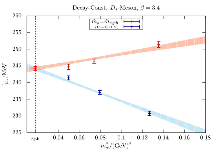 Figure 5
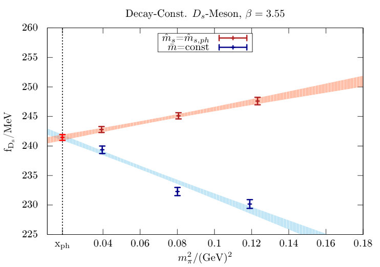 Figure 6
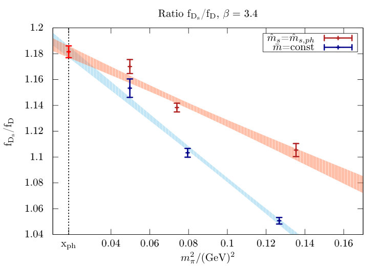 Figure 7
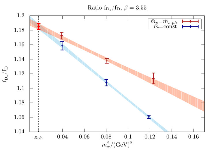 Figure 8
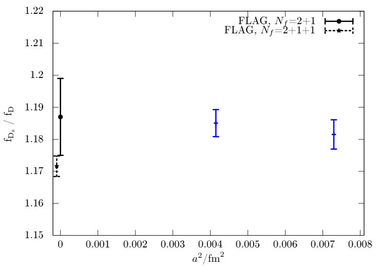 Figure 9
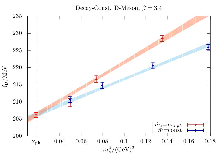 Figure 10
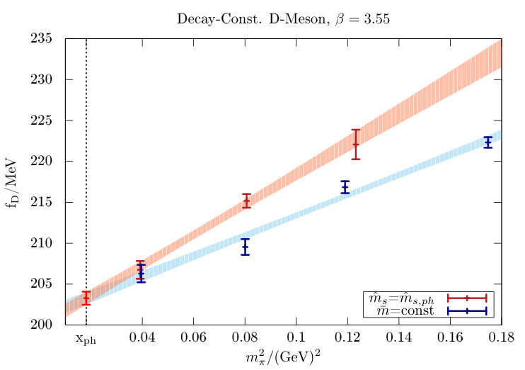 Figure 11
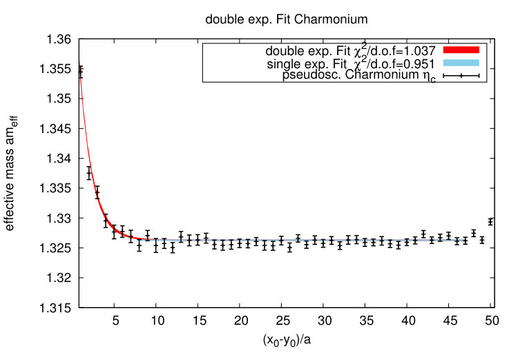 Figure 12
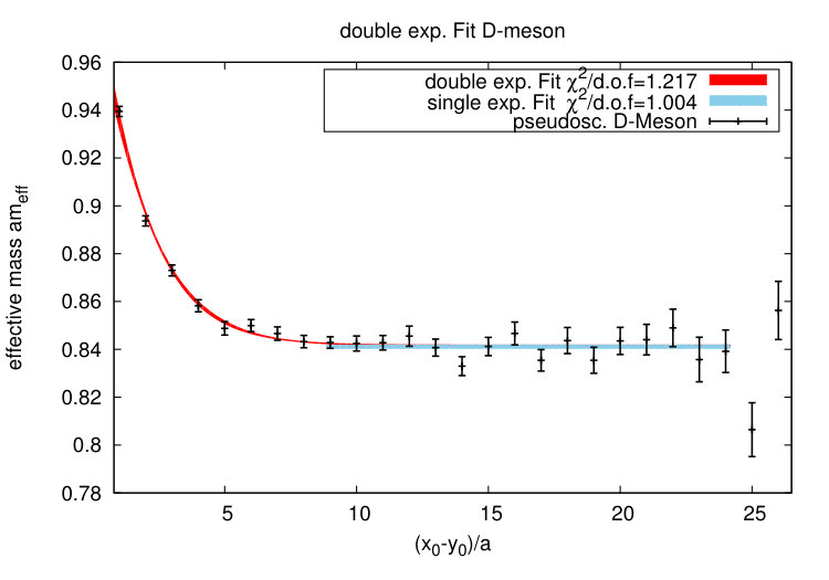 Figure 13
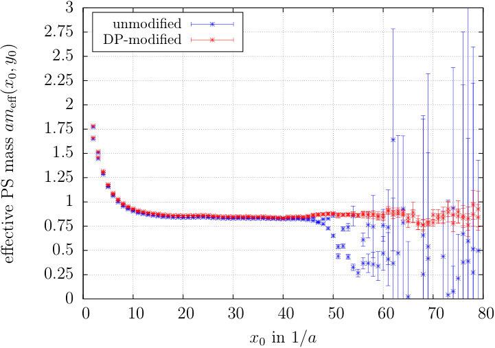 Figure 14
 Figure 15
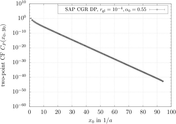 Figure 16
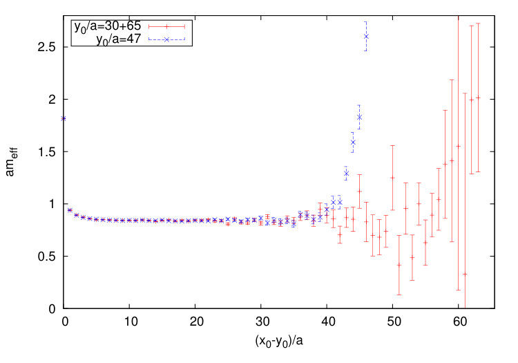 Figure 17
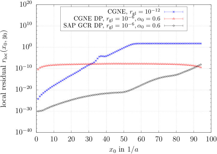 Figure 18
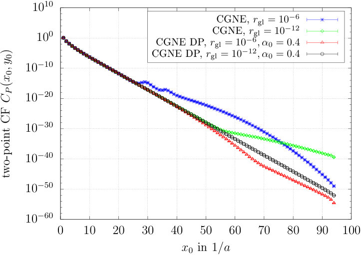 Figure 19
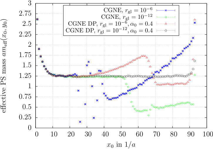 Figure 20
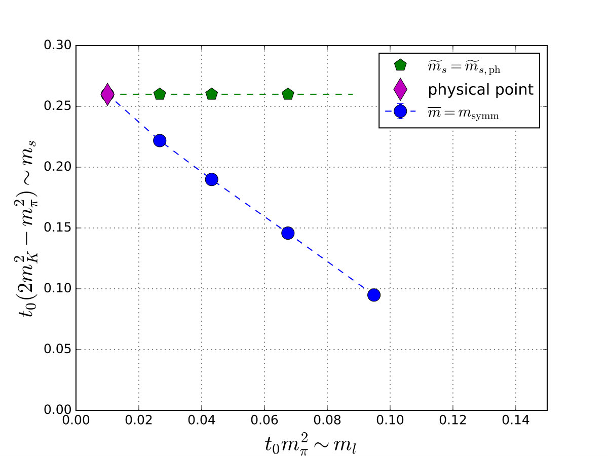 Figure 21
| trajectory | ensemble | |||||||
| [], | ||||||||
| H101 | 0.13675962 | 0.13675962 | 5.8 | 422 | 422 | 8000 | ||
| H102 | 0.136865 | 0.136549339 | 4.9 | 356 | 442 | 7988 | ||
| H105 | 0.13697 | 0.13634079 | 3.9 | 282 | 467 | 11332 | ||
| C101 | 0.13703 | 0.136222041 | 4.6 | 223 | 476 | 6208 | ||
| H107 | 0.136945665908 | 0.136203165143 | 5.1 | 368 | 549 | 6256 | ||
| H106 | 0.137015570024 | 0.136148704478 | 3.8 | 272 | 519 | 6212 | ||
| C102 | 0.1370508458 | 0.136129062556 | 4.6 | 223 | 504 | 6000 | ||
| [], | ||||||||
| H200 | 0.137 | 0.137 | 4.4 | 418 | 418 | 8000 | ||
| N203 | 0.13708 | 0.136840284 | 5.4 | 345 | 441 | 6172 | ||
| N200 | 0.13714 | 0.13672086 | 4.4 | 283 | 461 | 6800 | ||
| D200 | 0.1372 | 0.136601748 | 4.2 | 199 | 479 | 4000 | ||
| N204 | 0.137112 | 0.136575049 | 5.6 | 351 | 544 | 2000 | ||
| N201 | 0.13715968 | 0.136561319 | 4.5 | 284 | 522 | 6000 | ||
| D201 | 0.137207 | 0.136546436 | 4.1 | 198 | 499 | 4312 | ||
Peer Reviews
No public reviews on file for this paper yet. If you reviewed it on a platform where reviews are public (OpenReview, ICLR, NeurIPS, ICML), you can paste yours below so the community can read it here.
Videos
No videos yet. Explain this paper in a talk, walkthrough, or lecture? Add one.
Taxonomy
TopicsQuantum Chromodynamics and Particle Interactions · Particle physics theoretical and experimental studies · High-Energy Particle Collisions Research
Charmed pseudoscalar decay constants on
three-flavour CLS ensembles with open boundaries
MS-TP-16-36
Sara Collins, Kevin Eckert, Jochen Heitger, Stefan Hofmann and Wolfgang Söldner
(RQCD and ALPHA Collaborations)
aUniversität Regensburg, Institut für Theoretische Physik, D-93040 Regensburg, Germany
E-mail:
bWestfälische Wilhelms-Universität Münster, Institut für Theoretische Physik,
Wilhelm-Klemm-Straße 9, D-48149 Münster, Germany
E-mail Speaker.Speaker. [email protected],[email protected],[email protected]
[email protected],[email protected]
Abstract:
We determine the masses and pseudoscalar decay constants of D and mesons employing lattice QCD with non-perturbatively improved Wilson quarks and a tree-level Symanzik-improved gauge action. Our analysis is based on the large-volume ensembles using open boundary conditions, generated within the CLS effort. The status of results presented here covers two lattice spacings, fm and fm, and pion masses varied from 420 to 200 MeV. We also report on our implementation of distance preconditioning for the calculation of heavy quark propagators and discuss the impact of the resulting accuracy improvements on the extraction of charmed meson masses and decay constants. This is part of a continuing analysis by the RQCD and ALPHA Collaborations, aiming at a stable continuum extrapolation using several lattice spacings. To extrapolate to the physical masses, we follow both, the and the line in parameter space.
1 Introduction
Recent experiments at the LHC, BEPC II and KEK supply us with an abundance of spectroscopic information about charmed systems with ever improving measurements of the leptonic decay rates of D and mesons. In order to fully exploit this progress on the experimental side and to convert it into an amended determination of the CKM matrix entries \big{|}V_{\rm cq}\big{|}, , it must be complemented on the lattice QCD side with a more precise computation of the associated low-energy hadronic matrix elements, characterised by the pseudoscalar decay constants and , respectively. Charmed systems are challenging because of systematics, in particular, cutoff effects are generally significant. Therefore, all the more important is a fully controlled continuum extrapolation, . In this proceedings we describe our ongoing efforts in calculating the charmed pseudoscalar decay constants.
2 CLS ensembles and general computational setup
Our analysis is based on the Coordinated Lattice Simulations (CLS) ensembles generated with non-perturbatively improved Wilson-Sheikholeslami-Wohlert (clover) fermions and the tree-level improved Lüscher-Weisz gauge action, employing the open-source package openQCD [1].
Ensembles have been realised with lattice spacings in the range of (), aiming at a controlled extrapolation to the continuum limit [2, 3, 4]. Simulating with fm is possible through the use of open boundary conditions in the temporal direction, which avoids the problem of topological freezing as the continuum limit is approached [5, 6]. Readers, who are interested in the details regarding the algorithmic setup, are referred to Ref. [2]. Here, we only mention the use of twisted-mass reweighting for the two mass-degenerate light fermions [7], which prevents instabilities in the HMC algorithm due to near-zero modes of the Dirac operator, and the use of the rational approximation for simulating the strange quark. These algorithmic choices mean that the computation of observables, such as correlation functions, require reweighting, see Section 5.
So far we have analysed lattices with and corresponding to and , respectively [3]. For each -value, the physical point is approached in the light and strange quark mass plane following 2 trajectories — (i) keeping the average lattice quark mass ( 111Here we refer to the vector Ward identity masses, , where is the critical hopping parameter value at which the axial Ward identity mass in the symmetric limit, , vanishes.) fixed such that the sum of the renormalised quark masses is constant up to effects, and (ii) keeping the renormalised strange quark mass approximately constant. Figure 1 displays the two trajectories for , where the pion masses are varied from 422 down to 223 MeV. Simulations along the constant line, first proposed by the QCDSF Collaboration [8], start from the symmetric point with the strange (light) quark mass becoming heavier (lighter) towards the physical point. The quark mass dependence of hadron observables is given by Gell-Mann-Okubo expansions in powers of or, alternatively, can be described by SU(3) chiral perturbation theory (ChPT). For the second trajectory, SU(2) ChPT applies. See Ref. [3] for details on how an almost constant renormalised strange quark mass was achieved in this case. As will be demonstrated in Section 6, having two trajectories available enables the extrapolation to the physical point to be tightly constrained.
Table 1 provides further details of the ensembles entering our analysis. They exhibit large spatial volumes with high statistics; in particular, () is satisfied by all ensembles, and more than 4000 molecular dynamic units have been generated in each case (with the exception of ensemble N204, which is still in production). For open temporal boundaries, one needs large physical time extents, since discretisation effects and the propagation of scalar particles into the bulk mean that, in general, timeslices close to the boundaries need to be discarded. The lattice spacing is set by the gradient (resp. Wilson) flow scale , where we use , as determined by BMW Collaboration [9], together with -values from Refs. [2, 3]. Using the pion and kaon decay constants to set the scale, is discussed in Ref. [4]. The physical point is defined employing the combinations
[TABLE]
together with the pion and kaon masses in the isospin limit, and MeV, taken from the FLAG report [10]. We note that the starting value for the trajectory at the symmetric point, , was fixed by tuning , slightly above the physical value of . This choice was motivated by expected discretisation and {\cal O}\big{(}(m_{\rm s}-m_{\rm l})^{2}\big{)} effects in along the trajectory. In addition, the computation of involved in this tuning procedure was performed at unphysical quark mass. In the final analysis, the trajectory may be found to slightly miss the physical point. Mistunings of this kind, however, can still be accounted for later by slightly adjusting the results through reweighting or via a Taylor expansion (following Ref. [4]). We leave these considerations for future study.
3 Definition of observables
Let us explain our notation and the observables analysed. The pseudoscalar decay constants and are defined via the matrix elements of the axial vector current between and meson states and at momentum , respectively, and the vacuum, viz.
[TABLE]
where for quark flavours . In order to reduce leading discretisation effects to in the lattice simulation, we employ the improved axial operator
[TABLE]
The pseudoscalar interpolator is given by . The improvement coefficient has been determined non-perturbatively in Ref. [11]. Due to the breaking of chiral symmetry by Wilson-type fermions, the axial current must be renormalised in order to ensure that the continuum axial Ward identity
[TABLE]
is satisfied, where the (bare) vector Ward identity quark mass combinations read:
[TABLE]
The renormalisation factor is taken from the non-perturbative evaluation of Ref. [12]. The coefficient has been determined non-perturbatively in Ref. [13]. The same authors find to be consistent with zero in a preliminary analysis at . In order to perform a consistent analysis for both and 3.55, at present, we neglect the -term. Since the mass dependent corrections in Eq. (4) are anyway dominated by the term involving , this choice does not introduce a significant systematic uncertainty.
In the following, we restrict the analysis to zero-momentum and mesons, for which only the temporal component of the axial current needs to be considered. The matrix elements in Eq. (2) are extracted from the following two-point correlation functions:
[TABLE]
with the source and sink interpolating operators inserted at timeslices and , respectively. For sufficiently large time differences and , for a lattice of physical time extent 222For lattices with points in temporal direction, denotes the physical time extent. , these correlators behave as [4]
[TABLE]
where is the mass of a pseudoscalar meson containing a charm quark and an anti-quark of flavour . The (unrenormalised) lattice decay constant, , corresponds to , while the source-time dependent amplitude encapsulates the matrix element of the pseudoscalar operator and effects arising from the boundary close to the source. For sufficiently far from the boundary, holds.
In this preliminary analysis we place the source at large enough times such that boundary effects can be neglected. In order to gain statistics, three sources are chosen corresponding to , 47 and 65 for ensembles with and (see Table 1), while for , the sources are placed at , 47 and 68 for ensembles with , and at , 63 and 81 for those with . Ground-state dominance at small source-sink separations is realised by employing Wuppertal smearing [14, 15] with APE-smoothed links [16] to the pseudoscalar source and sink interpolators. Figure 2 displays typical effective masses for the D meson derived from the correlation function for the different source positions as a function of the sink-source time separation. For small , the results from the source in the center of the lattice () are compatible with those from the sources closer to the boundary (i.e., from the forward-propagating meson for and the backward-propagating meson for ), consistent with the absence of boundary effects. However, the latter are clearly evident for , as the sink time nears the boundary, while for and 65 the signal deteriorates before significant boundary effects are seen.
The pseudoscalar decay constant is extracted by fitting and to the functional forms given in Eq. (7), with independent of . The fitting procedure is discussed in Section 5. Alternative approaches, for instance, employing the axial Ward identity (i.e., PCAC) quark mass [17], will also be considered in the future. We remark that for pseudoscalar mesons containing a quark and an anti-quark of the same flavour, for which the statistical noise of the correlators is constant with varying source-sink separation, one can also place the source close to the boundary and consider ratios such as
[TABLE]
see Ref. [18] for details. When extracting the decay constant from the correlation functions, we wish to maximise the time range for the fit. However, there is a well known problem with numerical accuracy towards large time separations, when computing correlation functions involving propagators of heavy quarks. This issue is discussed in the next section along with the distance preconditioning procedure of Ref. [19], which can be adopted to alleviate such difficulties.
4 Distance preconditioning of heavy quark propagators
4.1 Motivation for distance preconditioning
When numerically inverting the Dirac operator, one has to pay special attention to the quality of the obtained solutions. Internally, the solver routine checks if the condition
[TABLE]
is satisfied, where is the discretized lattice Dirac operator, the bare quark mass in lattice units and the approximate solution at the -th iteration of the solver. denotes a source located on a single timeslice , while is the global residuum, i.e., indicating the numerical accuracy one likes to achieve. Contributions to the norm above are negligible for heavy quarks, if one considers large time separations between the source and the sink , because of the exponential decay of correlation functions . Solutions for large time extents thus become increasingly inaccurate in this case.
In order to improve the overall precision in our charm quark propagator computations, we have implemented the so-called “Distance Preconditioning” (DP) technique, first proposed in [19]. Rather than modifying the Dirac operator directly, as it was done in the original paper by de Divitiis et al., we included this preconditioning in the Dirac operator inversion via multiplication with a diagonal matrix ,
[TABLE]
with , corresponding to timeslice , and a (control) parameter . acts as unity matrix in spin, color and spatial coordinates. By this procedure, timeslices far away from the source are enhanced by a large exponential factor, which balances the rapid decay of the correlation function and ensures an accurate computation of the propagators even in the case of large quark masses (in lattice units) and very large time extents.
For our implementation, instead of numerically solving the un-preconditioned system
[TABLE]
we multiply it with from the left and rewrite as . The inversion to calculate the solution of the preconditioned system then becomes numerically much more stable, and to recover the original solution , it suffices to scale back with .
4.2 Numerical tests
We performed several exploratory tests on three different subsets of the CLS ensembles H105, H200 and U101. These low-statistic analyses (usually 25 to 200 configurations were included in the correlator measurements) served to explore the validity of the distance preconditioning technique for two different values of and different quark masses. The U101 subset was chosen because of its larger temporal lattice extent of .
Since there are contaminations from excited states near the source and excitations close to the boundary, the two-point functions defined in (6) have the general form
[TABLE]
where the first term mimics the ground state, the second one represents the first excited state with mass and the third term is the first excited boundary state with (see Ref. [4]). As one moves farther away from the boundary, the excited states become strongly suppressed, and the behaviour of the two-point functions is governed by the first term.
First tests of the distance preconditioning method were performed employing the normal-equation variant of the conjugate gradient solver (CGNE), because of its simplicity and numerical robustness. Figure 3 illustrates the numerical difficulties, as the correlator deviates from the expected behaviour (i.e., linear on a logarithmic scale) for large time separations . These results were obtained on ensemble H105 at with the correlation function averaged over two source positions and (DP-results were always generated utilising these source positions). The heavy-heavy correlator is evaluated for . With a loose global residual of the results for the unmodified CGNE solver (in blue) show an irregular behaviour already around timeslice . While this can still be partly improved via choosing a far smaller residual of order (in green), it is obvious that brute-force methods become unfeasible on lattices with larger time extent. The outcome can, however, be greatly improved by distance preconditioning: While the results for the DP-modified CGNE solver with and control parameter (red) already yield a modest improvement, those for (black) show a smooth and nearly perfect exponential decay over the whole range such that the effective pseudoscalar meson mass can be extracted along a wide plateau (the slight increase in at is likely due to boundary excited states back-propagating into the bulk).
In order to gain in computational speed, we also implemented the DP-method into another solver routine, namely, the domain-decomposition (SAP) preconditioned generalized conjugate residual solver (GCR). The left panel of Figure 4 shows the results for the local residual, defined as , for three different solver routines. While the CGNE solver (blue) shows substantial deviations between source and solution , this is neither the case for the DP-modified CGNE solver residual (red) that stays almost constant over the whole time extent, nor the DP-modified SAP GCR solver one (black), which stays well below . The right panel shows a representative result for H200 with and . If is chosen close to a value corresponding to , one can afford to set the global residual to even larger values, which helps to decrease the computational cost of the inversion further.
Finally, Figure 5 highlights the influence of DP on meson (left panel) and D meson (right panel) effective masses. While the light and strange quark systems were solved in all cases by a SAP-preconditioned GCR solver with local deflation (DFL), the charm quark inversion was performed either in the same way or via the DP-modified SAP GCR solver (red) for comparison. In the meson case, an increase in accuracy is clearly visible, as the plateau region extends farther into the bulk. For the D meson, the benefits of the DP-technique are less pronounced. Further studies based on higher statistics and devoted to finding optimal choices for and are certainly needed, given the promising results of our first numerical tests.
5 Analysis details
Since the tests of the distance preconditioning technique and its final implementation within our correlator measurement setup are still on-going, the results we present below were generated by solving the un-preconditioned linear system (Eq. 11) with a decreased residual (Eq. 9) of in the charm and in the strange and light quark propagator computations. With this choice of (global) residual for the charm quark inversion, the numerical problems discussed in the previous section can be seen in charmonium two-point functions at distances of around 60 timeslices from the source.
As mentioned in Section 2, we use twisted-mass reweighting for the light quarks and the rational approximation for the strange quark in the HMC. To correct to the proper distribution, we must reweight the physical observables (in this case, the two-point functions) with the associated reweighting factors:
[TABLE]
The twisted-mass () and rational approximation reweighting () factors are defined in Ref. [2] (Eqs. (3.2) and (3.5), respectively).
The analysis of the two-point functions proceeds by first making use of time-reversal symmetry and averaging and (, see Eq. 6) for the three source positions, e.g. and for at . In other words, we average the forward-propagating part of with the backward-propagating branch of , while for correlators with , we average the forward and backward propagating mesons. To extract the lattice pseudoscalar decay constant, we fit the averaged correlators for and simultaneously (i.e., four correlators in total) to the single-exponential forms in Eq. 7. Of course, this functional form is only valid in a region, where contamination from excited states has fallen below the noise and boundary effects as well as the numerical problems associated with the charm quark inversion are absent. As discussed in Section 3, the values of have been chosen to be sufficiently far away from the boundary. Effects from the opposite boundary and the numerical inversion problems are not significant when fixing the end point of the fit range to for the D meson and for the meson. In order to select the starting point of the fit interval, , we first estimated the contribution of the excited states by fitting the correlators to a double-exponential form. is then fixed to the point at which excited state contributions amount to less than one quarter of the statistical error of the correlation function. For example, for ,
[TABLE]
where and denote the amplitude and the mass of the first excited state, respectively, as determined by the fit, and denotes the statistical error of the correlator. Figure 6 illustrates this procedure. The lattice pseudoscalar decay constant is then extracted from a combination of the amplitudes of and (resulting from single-exponential fits between and ), in accordance with Eq. 7.
As the charm quark is partially quenched in our setup, we need to fix the corresponding hopping parameter () in our analysis. In a first step, on a subset of the available statistics, was estimated from the charmonium 1S spin-averaged mass . In order to maintain flexibility for possible adjustments later, the correlation functions were calculated with full statistics at two values of the hopping parameter, straddling the target ; these values were chosen by allowing the lattice spacing to vary by . was then determined on this full set by interpolating linearly in the inverse of the hopping parameter to the physical point, as given by the central value for . A linear interpolation is valid, since both -values for the “heavier” and “lighter” charm quark are close enough to the physical value. Employing the charmonium 1S mass introduces an unknown (although expected to be small) uncertainty, since we neglect the disconnected diagrams and possible flavour mixing. As an alternative, free from these systematics, we also determined utilising the spin-flavour-averaged 1S meson mass combination along the line, and the spin-averaged mass along the line. So far, the results for the interpolated decay constants, using fixed via either or and , were consistent within one standard deviation. In the future, we plan to base our final determination of the hopping parameter of the (valence) charm quark on and .
6 Preliminary results
The results presented in this section are preliminary and systematic errors arising from the uncertainty in the lattice spacing, fixing the charm quark mass, the renormalisation procedure, etc. are neglected. The statistical errors are estimated using a bootstrap analysis employing 500 samples. Let us first inspect the ratio of decay constants, , for which the renormalisation factor () drops out and also the contributions from the improvement terms partially cancel (see Eqs. (3) and (4)). Figure 7 shows our results for the ratio as a function of for and 3.55 (corresponding to and , respectively), consult Table 1 for the values of for each ensemble. We performed chiral extrapolations linear in along the trajectories of constant and simultaneously, enforcing the value at the physical point to be the same in both cases. As the dominant discretisation artefacts are of , we show the results for the two -values plotted against in Figure 8. The comparison with the recent FLAG averages for and [10] is promising.
The individual pseudoscalar D and meson decay constants are displayed in Figures 9 and 10. These depend on the renormalisation, and improvement has a big impact. If we focus on the meson, e.g., including the -improvement term in Eq. (4) causes an upward shift of the physical-point value of of about 35% for and 19% on the finer lattice. Similar shifts occur for . Most of the shift is due to the presence of the charm quark mass in . In contrast, for the ratio there is only a 1% shift when adding this improvement term, in line with the expectation that the impact of the charm quark largely cancels here. In the future, the chiral extrapolations will be investigated in more detail and, once results at additional lattice spacings have been analysed, a careful continuum limit extrapolation will also be performed.
7 Conclusions and outlook
Our ongoing simulations in the charmed meson sector of lattice QCD address the computation of the leptonic decay constants and . To reach a precision high enough to be relevant for theory inputs to global analyses in flavour physics phenomenology, among the next necessary steps are: (i) increase of statistics, inclusion of further ensembles and correcting the results for possible small mismatches of the constant physics condition, enabling a stable joint chiral and continuum extrapolation; (ii) a full budget of (statistical and systematic) errors, also accounting for their correlations. This will be carried out in the future.
Acknowledgments. We thank Gunnar Bali, Tomasz Korzec, Stefan Schaefer, Rainer Sommer and Nazario Tantalo for useful discussions. This work is supported by the Deutsche Forschungsgemeinschaft (DFG) through the grants GRK 2149 (Research Training Group “Strong and Weak Interactions – from Hadrons to Dark Matter”, K. E. and J. H.) and SFB/TRR 55 (S. C., S. H. and W. S.). We are indebted to our colleagues in CLS for the joint production of the gauge configurations. The authors gratefully acknowledge the Gauss Centre for Supercomputing e.V. for granting computer time on SuperMUC at the Leibniz Supercomputing Centre. Additional simulations were performed on the Regensburg iDataCool cluster and on the SFB/TRR 55 QPACE 2 and QPACE B computers [20, 21]. Some of the two-point functions were computed using the Chroma [22] software package, along with the locally deflated domain decomposition solver implementation of openQCD [1], the LibHadronAnalysis library and the multigrid solver implementation of Ref. [23]; our implementation of distance preconditioning (Section 4) is based on [24].
The reference list from the paper itself. Each links out to its DOI / PubMed record.
- 1[1] M. Lüscher and S. Schaefer, http://luscher.web.cern.ch/luscher/open QCD/ .
- 2[2] M. Bruno et. al. , JHEP 02 (2015) 043 [ 1411.3982 ].
- 3[3] RQCD Collaboration, G. S. Bali, E. E. Scholz, J. Simeth and W. Söldner, Phys. Rev. D 94 (2016), no. 7 074501 [ 1606.09039 ].
- 4[4] M. Bruno, T. Korzec and S. Schaefer, 1608.08900 .
- 5[5] M. Lüscher and S. Schaefer, JHEP 07 (2011) 036 [ 1105.4749 ].
- 6[6] M. Lüscher and S. Schaefer, Comput. Phys. Commun. 184 (2013) 519 [ 1206.2809 ].
- 7[7] M. Lüscher and F. Palombi, Po S LATTICE 2008 (2008) 049 [ 0810.0946 ].
- 8[8] W. Bietenholz et. al. , Phys. Lett. B 690 (2010) 436 [ 1003.1114 ].