Nuclear energy density functional and the nuclear alpha decay
Yeunhwan Lim, Yongseok Oh
TL;DR
This paper develops a method to predict alpha decay half-lives of heavy nuclei using nuclear energy density functional models to determine nucleon density profiles and fitting alpha potential parameters to experimental data.
Contribution
It introduces a novel approach combining energy density functional models with alpha decay data to predict unknown decay half-lives.
Findings
Accurately fitted alpha potential parameters to observed half-lives.
Predicted unknown alpha decay half-lives of heavy nuclei.
Estimated Q-values for unobserved alpha decays using the liquid droplet model.
Abstract
The nuclear decay of heavy nuclei is investigated based on the nuclear energy density functional, which leads to the potential inside the parent nucleus in terms of the proton and neutron density profiles of the daughter nucleus. We use the Skyrme force model, Gogny force model, and relativistic mean field model to get the nucleon density profiles inside heavy nuclei. Once the nucleon density profiles are determined, the parameters of the nuclear potential are fitted to the observed decay half-lives of heavy nuclei. This approach is then applied to predict unknown decay half-lives of heavy nuclei. To estimate the values of unobserved decays, we make use of the liquid droplet model.
Click any figure to enlarge with its caption.
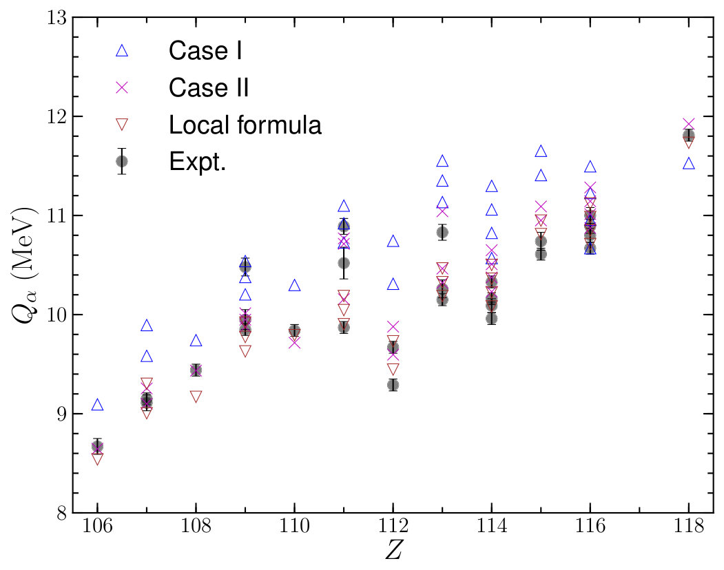 Figure 1
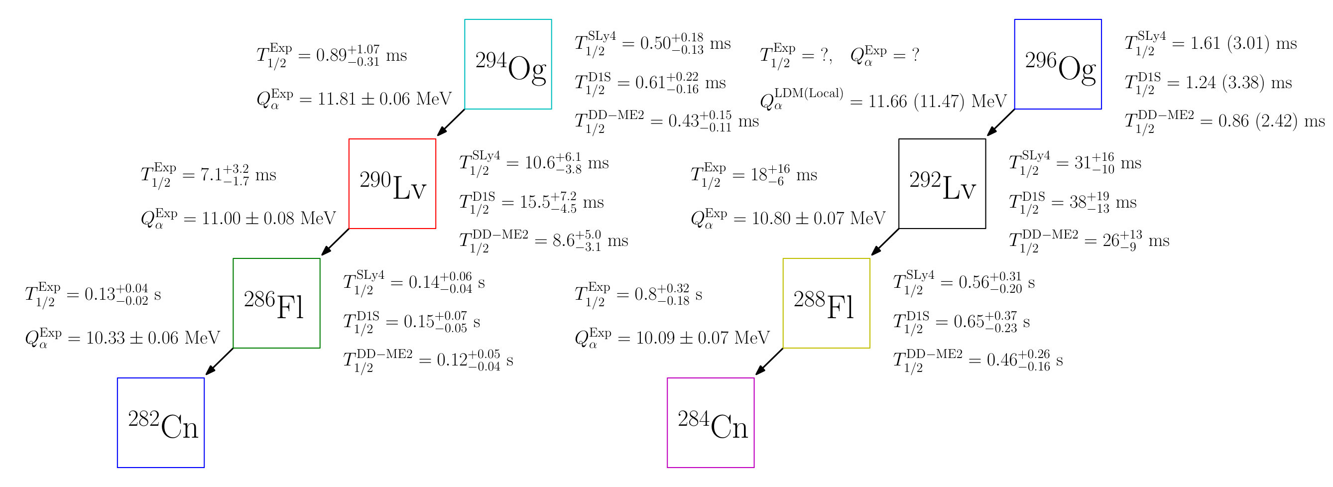 Figure 2
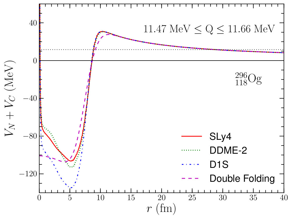 Figure 3
| Case I | Case II | Unit | |
| 16.125 | 16.370 | MeV | |
| 0.155 | 0.155 | fm-3 | |
| 1.256 | 1.300 | MeV fm-2 | |
| 4.0 | 3.7 | ||
| 60.00 | 25.48 | ||
| 31.818 | 32.471 | MeV | |
| 250.00 | 226.389 | MeV | |
| 5.458 | 6.232 | MeV | |
| 5.807 | 11.760 | MeV | |
| 1.265 | MeV | ||
| MeV | |||
| MeV | |||
| MeV | |||
| 184 | 168 | ||
| RMSD | 1.144 | 0.218 | MeV |
| RMSD | |||||
|---|---|---|---|---|---|
| Parameter | SLy4 | D1S | DD-ME2 | Unit |
|---|---|---|---|---|
| MeV fm3 | ||||
| MeV fm5 | ||||
| MeV fm6+ϵ | ||||
| MeV fm5 | ||||
| MeV fm5 | ||||
| (MeV) | Reference | |||||
|---|---|---|---|---|---|---|
| ms | ms | ms | ms | OULA06 | ||
| ms | ms | ms | ms | OULA04b | ||
| ms | ms | ms | ms | OULA04b | ||
| ms | ms | ms | ms | OULA06 | ||
| ms | ms | ms | ms | OULA06 | ||
| ms | ms | ms | ms | OULA04 ; OUDL05 | ||
| ms | ms | ms | ms | OULA04 ; OUDL05 | ||
| s | s | s | s | OULA04b | ||
| s | s | s | s | OULA04b | ||
| s | s | s | s | OULA06 | ||
| s | s | s | s | OULA06 | ||
| s | s | s | s [] | OULA04 ; OUDL05 | ||
| ms | ms | ms | ms | OULA04 ; OUDL05 | ||
| ms | ms [] | ms [] | ms [] | OULA07 | ||
| s | ms | s | s | OULA04b | ||
| s | s | s | s | OULA06 | ||
| s | s [] | s [] | s [] | OULA04 ; OUDL05 | ||
| ms | ms [] | ms [] | ms [] | OULA04 ; OUDL05 | ||
| ms | ms [] | ms [] | ms [] | OULA07 | ||
| s | s | s | s | OULA06 | ||
| s | s [] | s [] | s [] | OULA04 ; OUDL05 | ||
| ms | ms [] | ms [] | ms [] | OULA04 ; OUDL05 | ||
| ms | ms [] | ms[] | ms [] | OULA07 | ||
| s | s | s | s | OULA06 | ||
| s | s [] | s [] | s [] | OULA04 ; OUDL05 | ||
| s | s [] | s [] | s [] | OULA07 | ||
| min | min [] | min [] | min [] | OULA06 | ||
| RMSD | - | - |
| Nuclei | (MeV) | (s) | (s) | (s) | (MeV) | (s) | (s) | (s) |
|---|---|---|---|---|---|---|---|---|
| LDM | Local formula | |||||||
| (122, 307) | 12.594 | 12.289 | ||||||
| (122, 306) | 12.729 | 12.420 | ||||||
| (122, 305) | 12.853 | 12.550 | ||||||
| (122, 304) | 12.986 | 12.679 | ||||||
| (122, 303) | 13.108 | 12.807 | ||||||
| (122, 302) | 13.239 | 12.935 | ||||||
| (121, 306) | 12.114 | 11.853 | ||||||
| (121, 305) | 12.250 | 11.985 | ||||||
| (121, 304) | 12.367 | 12.117 | ||||||
| (121, 303) | 12.511 | 12.248 | ||||||
| (121, 302) | 12.636 | 12.378 | ||||||
| (121, 301) | 12.769 | 12.508 | ||||||
| (120, 304) | 11.790 | 11.546 | ||||||
| (120, 303) | 11.918 | 11.679 | ||||||
| (120, 302) | 12.055 | 11.812 | ||||||
| (120, 301) | 12.181 | 11.944 | ||||||
| (120, 300) | 12.317 | 12.076 | ||||||
| (120, 299) | 12.442 | 12.207 | ||||||
| (119, 298) | 11.973 | 11.772 | ||||||
| (119, 297) | 12.109 | 11.904 | ||||||
| (119, 296) | 12.234 | 12.036 | ||||||
| (119, 295) | 12.368 | 12.167 | ||||||
| (119, 294) | 12.492 | 12.297 | ||||||
| (119, 293) | 12.625 | 12.427 | ||||||
| (118, 298) | 11.393 | 11.197 | ||||||
| (118, 297) | 11.522 | 11.332 | ||||||
| (118, 296) | 11.660 | 11.466 | ||||||
| (118, 295) | 11.787 | 11.600 | ||||||
| (118, 294) | 11.924 | 11.733 | ||||||
| (118, 293) | 12.050 | 11.865 | ||||||
| (117, 298) | 10.779 | 10.920 | ||||||
| (117, 297) | 10.920 | 10.749 | ||||||
| (117, 296) | 11.051 | 10.886 | ||||||
| (117, 295) | 11.192 | 11.023 | ||||||
| (117, 294) | 11.321 | 11.158 | ||||||
| (117, 293) | 11.460 | 11.293 |
Peer Reviews
No public reviews on file for this paper yet. If you reviewed it on a platform where reviews are public (OpenReview, ICLR, NeurIPS, ICML), you can paste yours below so the community can read it here.
Videos
No videos yet. Explain this paper in a talk, walkthrough, or lecture? Add one.
Nuclear energy density functional and the nuclear decay
Yeunhwan Lim
Cyclotron Institute and Department of Physics and Astronomy, Texas A&M University, College Station, Texas 77843, USA
Yongseok Oh
Department of Physics, Kyungpook National University, Daegu 41566, Korea
Asia Pacific Center for Theoretical Physics, Pohang, Gyeongbuk 37673, Korea
Abstract
The nuclear decay of heavy nuclei is investigated based on the nuclear energy density functional, which leads to the potential inside the parent nucleus in terms of the proton and neutron density profiles of the daughter nucleus. We use the Skyrme force model, Gogny force model, and relativistic mean field model to get the nucleon density profiles inside heavy nuclei. Once the nucleon density profiles are determined, the parameters of the nuclear potential are fitted to the observed decay half-lives of heavy nuclei. This approach is then applied to predict unknown decay half-lives of heavy nuclei. To estimate the values of unobserved decays, we make use of the liquid droplet model.
pacs:
23.60.+e, 21.30.-x, 21.65.Ef, 27.90.+b
I Introduction
The synthesis of unknown heavy nuclei has been spotlighted for last decades with the development of new facilities for rare isotope accelerators Moller16 ; GS16 ; GGW16 . In particular, the structure of neutron-rich heavy nuclei is expected to shed light on our understanding of nuclear structure in isospin asymmetric nuclear matter and it will give insight on the structure of neutron stars and the process of nuclear synthesis during the evolution of stars GLM07 . Therefore, it can be a test ground for various issues of nuclear physics such as nuclear density functional, strong nuclear interactions, various decay processes, r-p process, etc, which makes it one of the most exciting topics in low energy nuclear physics OST17 . The formation of such heavy nuclei is identified through their decay processes such as the decay, decay, and spontaneous fission VS66b . The competition between these decay processes is reflected in branching ratios, and, in fact, the heavy nuclei with the atomic number were found to rarely survive for a few minutes AWWK12 ; WAWK12 .
The study on the nuclear decay process has a very long history, as it is one of the major decay processes of nuclei Mang64 ; VS66b . In particular, the formation of a new heavy nuclide would be mostly identified through its decay chains Oganessian07 ; MMKH12 ; KYDA14 . Modern approaches for theoretical understanding of the nuclear decay are based on effective nuclear interactions such as the square well potential model BMP91 ; BMP92 , potential model BMP92b , unified fission model DZGWP10 , double-folding model RSB05 ; SCB07 ; RSB08 , and so on.
The most important factor in the decay process of heavy nuclei is the accurate information on the value for the decay process, which reflects the structure of heavy nuclei through binding energy. The importance of the value in the decay lifetime can easily be found in the Geiger-Nuttall law GN11 and its improved version of Viola and Seaborg VS66b .111 For example, in the case of the alpha decay of , a difference of 0.1 MeV in the value of the reaction, where MeV, results in about a factor of 1.7 difference in the calculated half-life of \nuclide[212]Po.
The next most sensitive factor in the determination of the decay width is the nucleon distribution inside the daughter nucleus, which determines the potential. Since the -decay is basically a quantum tunneling effect, the exact positions of the classical turning points and the profile of the barrier, i.e., its height and width, are essential parts for the estimation of the decay lifetime. Therefore, the information on the nuclear potential felt by the cluster inside the parent nucleus is important to estimate the decay width. Furthermore, the Coulomb potential is responsible for the repulsive potential barrier together with the angular momentum barrier, so the potential shape due to the proton distribution in the daughter nucleus has a nontrivial role in the decay process. The purpose of the present work is to go beyond a simple model approach for the potential by developing a more realistic potential based on nucleon density profiles for estimating decay half-lives.
In the present work, we calculate the decay half-lives of heavy nuclei within the Wentzel-Kramers-Brillouin (WKB) approximation by calculating the nuclear potential felt by the cluster using phenomenological nuclear force models. The nuclear potential form for the cluster is obtained from the Skyrme-type interaction as prescribed in Ref. SLHO15 , which requires the proton and neutron distribution functions as inputs. We then use the Skyrme SLy4 model CBHMS98 and Gogny D1S model BGG91 as non-relativistic models and the relativistic mean-field DD-ME2 model LNVR05 as well. For the values of the decay processes, we use the experimental data whenever available, and, if not, we make use of the liquid droplet model (LDM) elucidated in Ref. SPLE04 .
This paper is organized as follows. In Sec. II, we review the LDM to calculate the binding energy to be used when the experimental value is not known. The Coulomb diffusion and exchange terms are included as well as the pairing and shell corrections, which gives a better fitting to existing data. In the shell corrections, we use the last magic number as a free variable to minimize the root-mean-square deviation of total binding energy. We also check the values using the phenomenological formula as a function of isospin asymmetry , with , as in Ref. DZGWP10 . Section III briefly explains nuclear models to find the density profiles of nucleons inside nuclei, and we construct the effective nuclear potential for the cluster. The parameters of the effective potential for each model of nucleon density distribution are determined. Our results are presented in Sec. IV and compared to experimental data. The predictions on the unobserved decays of heavy nuclei are given as well. We summarize and conclude in Sec. V.
II Nuclear models
The value plays an important role to determine the lifetime of the decay as it determines the assaulting frequency of the particle for a given potential well. It also sets the penetration width for quantum tunneling. In the estimation of decay lifetimes, we use the empirical values, if available. However, for unobserved decay processes, we have to resort to model predictions on the binding energy. In this Section, we review the LDM that will be used in the present work.
II.1 Liquid Droplet Model
To estimate the unknown binding energies of heavy nuclei, we make use of the LDM with some modifications as prescribed in Refs. MS69 ; SPLE04 . In general, heavy nuclei are neutron-rich and the neutron skin is likely to exist on the surface. For example, the neutron skin thickness of \nuclide[208]Pb was investigated with the electric dipole response TPVF11 , the parity radius experiment (PREX) PREX12 ; HAJR12 , and, more recently, through coherent photoproduction CB14 . All numerical calculations using Skyrme-Hartree-Fock, Gogny, and relativistic mean field models show the out-layer of neutrons in the neutron-rich heavy nuclei. Thus, it is natural to include the neutron skin effects in LDM. The binding energy in the LDM for a nucleus of () is given as SPLE04
[TABLE]
where is the binding energy per baryon of infinite nuclear matter, is the number of neutrons in the neutron skin on the surface, is the radius of the nucleus, is the surface tension as a function of neutron chemical potential . is the Coulomb energy, is the pairing energy, and includes the shell corrections.
In this model, is a phenomenological energy function, which reads
[TABLE]
where is the binding energy per nucleon, is the nuclear symmetry energy, and is the nuclear incompressibility of symmetric nuclear matter at nuclear saturation density . Here, and are defined as
[TABLE]
The surface tension is a function of , and we find that the simple expansion of is not a good approximation for highly neutron-rich nuclei. Therefore, we use the form suggested in Refs. RPL83 ; Lim12 , which reads
[TABLE]
The parameters , , and will be determined later.
The Coulomb energy contribution to the total mass is obtained from the classical Coulomb interaction, the Coulomb diffusion term, and the exchange term. It is then written as
[TABLE]
where ( is the surface diffuseness parameter SPLE04 and is the average radius of the nucleus. The general expression for the pairing energy in LDM reads
[TABLE]
where the pairing energies for protons and neutrons are treated separately, since neutron-rich nuclei would have higher single particle energy of the last-filled neutron than the one for protons.
For the shell contribution to the total binding energy, we follow the prescription of Duflo and Zuker DZ94 ; DV09 , which writes the shell correction as
[TABLE]
where , , , and are parameters to be determined, and
[TABLE]
Here, and are the valence numbers of neutrons and protons, respectively, i.e., the minimal difference for neutron and proton numbers from the magic numbers, 2, 8, 20, 28, 50, 82, 126, and 184 (or 168). For example, for \nuclide[56]Fe, we obtain and . () is the degeneracy number, i.e, the interval of the magic numbers adjacent to the neutron (proton) number. For instance, in the case of \nuclide[56]Fe, the nearest two magic numbers for are and , which then leads to . Finally, and are the complementary valence numbers for neutrons and protons, respectively, and their explicit forms are
[TABLE]
Again, for \nuclide[56]Fe, we have .
In the present work, we will work with two parameter sets as given in Table 1. The parameters of case I are obtained by fitting to the experimentally known binding energies of 2336 nuclei. Therefore, this corresponds to a global fitting. On the other hand, since we are considering decays of neutron-rich heavy nuclei, it may be useful to focus on heavy nuclei for that purpose. Thus the second parameter set is found by using the measured values of heavy nuclei with . We use 100 data points for finding the parameters set of case II. Note that in Table 1 is the 8th magic number in the LDM parameterization with each parameter set.
Once the masses of nuclei are evaluated by Eq. (1), we can calculate the value for decay through MRDT06
[TABLE]
where MeV. The values for and are ( MeV, ) for nuclei of , and ( MeV, ) for nuclei of .
II.2 Local formula for
Considering heavy nuclei with and , Dong et al. DR08 ; DZGWP10 developed a local mass formula for nuclei with large and values. Using the Taylor expansion, it leads to the expression of the local value including shell effects as
[TABLE]
where , , , , and are parameters to be fitted. Note that the pairing effects are neglected since the semi-classical formula gives almost the same contribution to the total binding energy for both parent and daughter nuclei and it does not cause a change in the value. Since our goal is to compute the half-lives of super heavy nuclei through decay processes, we obtain the parameters in Eq. (11) with the measured values for nuclei with . The resulting parameters are shown in Table 2.
Figure 1 shows the values obtained from the LDM with Eq. (10) and those from the local formula of Eq. (11). It is found that the case II and the local formula give more reliable results than case I on the measured values.
III Potential for the cluster
In the cluster model, the nuclear decay is described as a quantum tunneling effect. Once the energy, i.e., the value, of the reaction is determined, the next step is to find the potential for the cluster inside the parent nucleus. In this Section, we discuss how we use phenomenological models for constructing the potential for the cluster.
III.1 Potential form
In the cluster model, the particle is already formed in the parent nucleus and it penetrates the potential barrier to cause the decay process. Therefore, the estimation of lifetimes requires the information on the potential of the cluster created by the core nucleus, i.e., the daughter nucleus after decay.
The cluster potential can be decomposed as
[TABLE]
where is the nuclear potential for the cluster, is the Coulomb potential provided by the protons of the core nucleus, and is the centrifugal potential arising from the relative orbital angular momentum between the particle and the core nucleus. In principle, the nuclear potential of the particle would be computed if the interactions between nucleons inside a nucleus is completely known. However, it is certainly beyond the scope of the present work, and we invoke the Skyrme force model to get the form of . Then, as described in Ref. SLHO15 , takes the form of
[TABLE]
where with () being the density distribution of neutrons (protons). This model contains 6 parameters, namely, , , , , , and . These parameters will be determined by fitting to the empirical data for decay half-lives of heavy nuclei and will be discussed in the next subsection. Furthermore, the nuclear potential in Eq. (13) is controlled by the density distribution of nucleons, which should be provided by microscopic models for nuclear structure.
Once the nucleon distribution is known, the Coulomb potential term can be calculated through
[TABLE]
The centrifugal potential is written as
[TABLE]
where is the reduced mass, and the Langer modification factor Langer37 is adopted.
III.2 Nucleon density profiles
Since the cluster potential of Eq. (13) requires the information on the density profile of the daughter nucleus, we rely on microscopic models for nuclear structure. In the present work, we consider the Skyrme SLy4 (zero-range) CBHMS98 and the Gogny D1S (finite-range) BGG91 models as non-relativistic approaches and the relativistic mean-field interaction DD-ME2 model of Ref. LNVR05 as a relativistic approach.
The Skyrme force model is constructed based on nucleon-nucleon interactions having dependence on the relative momentum and density, which reads
[TABLE]
where is the spin exchange operator, and are the Pauli spin matrices. Here, and are the relative momenta of two nucleons before and after interaction, respectively, and is the strength of the spin-orbit coupling. There are many versions of the parameter set and, in the present work, we use the SLy4 model compiled in Ref. CBHMS98 .
Compared with the Skyrme force model, the Gogny force assumes finite-range nucleon-nucleon interactions and zero-range multi-body forces, which leads to DG80
[TABLE]
where is the isospin exchange operator. We use the parameter values known as the D1S model in Ref. BGG91 .
For nucleon density distribution, we also use a relativistic mean-field model of Refs. LNVR05 ; NPVR14 , which gives a satisfactory description for the properties of finite nuclei. In this model, the relativistic Lagrangian density is given by
[TABLE]
where , , and are the field strength tensors of the vector meson field , the isovector vector meson field , and the photon field , respectively. Note that the coupling constants of mesons to the nucleon are density-dependent so as to reproduce the properties of nuclear matter and finite nuclei. In the present work, we adopt the parameter set given as the DD-ME2 model in Ref. LNVR05 .
Within the Skyrme and Gogny force models, we solve Schrödinger-like equations to obtain the density profile of a nucleus. On the other hand, in the relativistic mean field model, we solve the Dirac equation to get the density profile for a given nucleus. Once the density profile is known, one can find the potential for each nucleus and the decay lifetime can be computed. Since the potential in Eq. (12) contains 6 parameters, we determine these parameters to the experimental data for the alpha decays of even-even nuclei () as we have done in Ref. SLHO15 . Table 3 shows the parameters for the nuclear potential determined in this manner. The potential parameters for each model are found to have similar magnitudes except the case of , which is correlated to the value of . The term is related with the multi-body force and we choose in the Gogny D1S model reflecting the original value in the Gogny interaction.
IV Results
Equipped with the potential obtained in the previous section, the -decay half-lives of heavy nuclei can be estimated in the standard way by using the WKB approximation. The half-life of the nuclear decay is related to the decay width by
[TABLE]
where the decay width is given by
[TABLE]
Here, is the preformation factor which illustrates the probability of particle in the parent nuclei, and is the assaulting frequency of the trapped particle between two turning points and . In this calculation, we use and the explicit expression for can be found, for example, in Ref. SLHO15 . The distance between and , i.e., , represents the penetration width of the barrier through which particle passes. corresponds to the wave number of the particle inside the potential barrier,
[TABLE]
with being the reduced mass of the system.
The heavy nuclei under study in the present work are neutron-rich but are located on the neutron-deficient side of beta-stability. Thus, decay does not occur for these nuclei. Table 4 shows our results on the observed decay half-lives of heavy nuclei. Our results are obtained with the three models for nuclear density profiles and are compared with experimental data. The theoretical uncertainties shown in the table come from those of the experimental values. The obtained half-lives depend on the relative orbital angular momentum . We assume for even-even decay cases but we allow the variation of in other types of decay processes. The value of which minimizes the difference with the experimental data for the half-life is explicitly shown in Table 4. The results for half-lives without the value of are obtained with . Compared with the previous results given in Ref. SLHO15 which used a simple Fermi density profile, using realistic proton distribution improves the rms deviation (RMSD) in decay lifetimes as shown in the table, which is defined by
[TABLE]
where is the total number of data. This indicates that the density profile of the neutron-rich heavy nuclei deviates from the simple Fermi density profile and its effect should be considered to get more realistic results.
Presented in Table 5 are our predictions on the half-lives of unobserved decays of superheavy elements. In this case, the values are estimated by using the LDM and the local formula as described in Sec. II. We assume for simplicity as there is no information on these processes.222If , the potential barrier width becomes larger than the case of and the lifetime becomes longer. For example, when MeV, if we use the Gogny D1S model, the enhancement factors for the half-life become , , , , and as we increase the value of from to . Other models give similar results. Note that the half-lives from the D1S calculation are longer than the ones from SLy4 and DD-ME2 calculations. We found that this is mostly caused by the differences in parameters given in Table 3.
Figure 2 shows one of the most important decay chains of superheavy nuclei, namely, the decay chains of \nuclide[294][118]Og and \nuclide[296][118]Og. Our results successfully explain the decay lifetimes in these two decay channels compared with experimental results. The decay of \nuclide[296][118]Og is yet to be discovered and the half-lives for this decay given in Fig. 2 are our predictions. It should be noticed that the half-lives shown in Fig. 2 are calculated from the nuclear decay but the actual half-lives should be determined through the competition with the spontaneous fission process. For example, in the case of \nuclide[286]Fl, although the measured half-life is s, the branching ratio of the -decay is about 60% OU15 ; OU15b , which makes the -decay half-life close to 0.22 s.
Figure 3 shows the potentials, , used to calculate the half-life of \nuclide[296][118]Og in this work. The dotted line indicates the -values obtained in this work. The double folding potential is presented by the dashed line for comparison Mohr16 . This shows that, although the details of the potentials in each model are quite different inside the nucleus, the barrier widths corresponding to the obtained values are relatively close to each other. The sightly lower barrier in Ref. Mohr16 is compensated by a preformation factor of 0.09, finally leading to half-lives close to each other.
V Summary and Conclusion
In this paper, we have investigated the nuclear decays of heavy nuclei based on nuclear energy density functional. We use a Skyrme-type force model to get the nuclear potential of the particle inside a nucleus as a functional of proton and neutron density profiles of the daughter nucleus. These nucleon density profiles are obtained from the Skyrme SLy4, Gogny D1S, and relativistic mean-field DD-ME2 models. The parameters of the nuclear potential of the are fitted for each density profile model to measured decay half-lives of heavy nuclei. The results show that this approach improves the previous results reported in Ref. SLHO15 , by reducing the RMS deviation from 0.238 to . In particular, we found that the Gogny D1S gives a better description among the models considered in the present work.
Once all the parameters are fixed, we apply the model to predict half-lives of unobserved decays to get the estimations shown in Table 5. One interesting quantity is the half-life of \nuclide[296][118]Og as there are attempts to synthesize this nuclide Sobiczewski16 . Our predictions on this decay are also shown in Fig. 2, which shows our estimation of the value as MeV and MeV. Our predictions on the half-life of the decay of this nuclide is in the range of , which is in good agreement with the predictions of Ref. Sobiczewski16 that gives based on realistic mass formulas and with the prediction of Ref. Mohr16 which obtained 0.825 ms using the double-folding potential model. (See also Refs. SPN16 ; Manjunatha16 .)
In the present work, we assumed that the potential for the is isotropic. However, in the case of heavy nuclei, the deformation effects should be included, in particular, to understand its fine structure DIL92 ; NR10 . Therefore, improving the present model by including deformation and other microscopic effects would be desired for a better understanding of nuclear decays of superheavy nuclei.
Acknowledgements.
We are grateful to P. Papakonstantinou for providing us with density profiles of nuclei obtained in the Gogny force model. We also thank P. Mohr for providing his double folding potential for decay and many suggestions for this work. The work of Y.O. was supported by Kyungpook National University Bokhyeon Research Fund, 2015.
The reference list from the paper itself. Each links out to its DOI / PubMed record.
- 1(1) P. Möller, The limits of the nuclear chart set by fission and alpha decay, EPJ Web Conf. 131 , 03002 (2016).
- 2(2) A. Gade and B. M. Sherrill, NSCL and FRIB at Michigan State University: Nuclear science at the limits of stability, Phys. Scripta 91 , 053003 (2016).
- 3(3) J. Gerl, M. Górska, and H. J. Wollersheim, Towards detailed knowledge of atomic nuclei — the past, present and future of nuclear structure investigations at GSI, Phys. Scripta 91 , 103001 (2016).
- 4(4) H. Grawe, K. Langanke, and G. Martínez-Pinedo, Nuclear structure and astrophysics, Rep. Prog. Phys. 70 , 1525 (2007).
- 5(5) Yu . Ts . Oganessian, A. Sobiczewski, and G. M. Ter-Akopian, Superheavy nuclei: from predictions to discovery, Phys. Scripta 92 , 023003 (2017).
- 6(6) V. E. Viola, Jr. and G. T. Seaborg, Nuclear systematics of the heavy elements - II. Lifetimes for alpha, beta and spontaneous fission decay, J. Inorg. Nucl. Chem. 28 , 741 (1966).
- 7(7) G. Audi, M. Wang, A. H. Wapstra, F. G. Kondev, M. Mac Cormick, X. Xu, and B. Pfeiffer, The Ame 2012 atomic mass evaluation (I). Evaluation of input data, adjustment procedures, Chin. Phys. C 36 , 1287 (2012).
- 8(8) M. Wang, G. Audi, A. H. Wapstra, F. G. Kondev, M. Mac Cormick, X. Xu, and B. Pfeiffer, The Ame 2012 atomic mass evaluation (II). Tables, graphs and references, Chin. Phys. C 36 , 1603 (2012).