The rigorous derivation of the linear Landau equation from a particle system in a weak-coupling limit
Nicol\`o Catapano

TL;DR
This paper rigorously derives the linear Landau equation from a particle system with short-range interactions in a weak-coupling regime, bridging microscopic dynamics and kinetic equations.
Contribution
It provides a rigorous derivation of the linear Landau equation from particle interactions, connecting Boltzmann and Landau equations in a novel weak-coupling setting.
Findings
Asymptotic equivalence between one-particle marginal and linear Boltzmann solution
Derivation of Landau equation via grazing collision limit
Validation of kinetic equations from particle systems
Abstract
We consider a system of N particles interacting via a short-range smooth potential, in a intermediate regime between the weak-coupling and the low-density. We provide a rigorous derivation of the Linear Landau equation from this particle system. The strategy of the proof consists in showing the asymptotic equivalence between the one-particle marginal and the solution of the linear Boltzmann equation with vanishing mean free path.Then, following the ideas of Landau, we prove the asympotic equivalence between the solutions of the Boltzmann and Landau linear equation in the grazing collision limit.
Click any figure to enlarge with its caption.
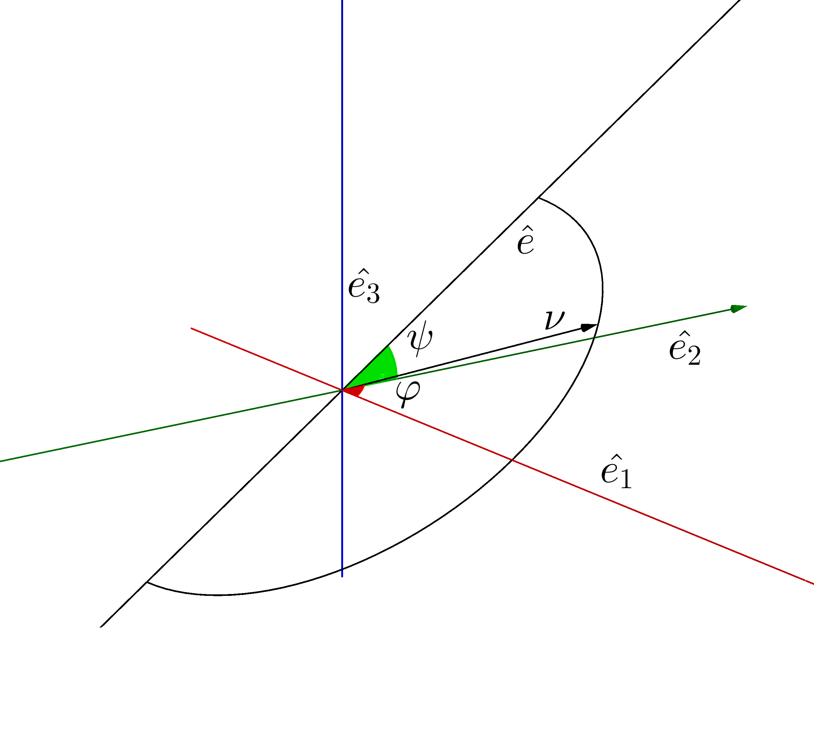 Figure 1
Peer Reviews
No public reviews on file for this paper yet. If you reviewed it on a platform where reviews are public (OpenReview, ICLR, NeurIPS, ICML), you can paste yours below so the community can read it here.
Videos
No videos yet. Explain this paper in a talk, walkthrough, or lecture? Add one.
Taxonomy
TopicsGas Dynamics and Kinetic Theory · Advanced Thermodynamics and Statistical Mechanics · Cold Atom Physics and Bose-Einstein Condensates
The rigorous derivation of the Linear Landau equation from a particle system in a weak-coupling limit
N. Catapano
Dipartimento di Matematica, Università di Roma “La Sapienza”, P.le A. Moro, 5, 00185 Roma, Italy.
E-mail: [email protected]
Abstract
We consider a system of N particles interacting via a short-range smooth potential, in a weak-coupling regime. This means that the number of particles goes to infinity and the range of the potential goes to zero in such a way that , with diverging in a suitable way. We provide a rigorous derivation of the Linear Landau equation from this particle system. The strategy of the proof consists in showing the asymptotic equivalence between the one-particle marginal and the solution of the linear Boltzmann equation with vanishing mean free path. This point follows [3] and makes use of technicalities developed in [16]. Then, following the ideas of Landau, we prove the asympotic equivalence between the solutions of the Boltzmann and Landau linear equation in the grazing collision limit.
Contents
1 Introduction
1.1 The Boltzmann-Grad limit
In kinetic theory a gas is described by a system of small indistinguishable interacting particles. The evolution of this system is quite complicated since the order of particles involved is quite large. For this reason it is interesting to consider the system from a statistical point of view. The starting point is a system of particles having unitary mass and moving in a domain . These particles can interact by means of a short-range radial potential . The microscopic state of the system is given by the position and velocity variables denoted by and , where are respectively position and velocity of the i-th particle. The time is denoted by . Throughout the paper we will use bold letters for vectors of variables.
Let be a parameter denoting the ratio between typical macroscopic and microscopic scales, say the inverse of the number of atomic diameters necessary to fill a centimeter. If we want a macroscopid description of the system it is natural to introduce macroscopic variables defined by
[TABLE]
where are the macroscopic position and is the macroscopic time variable. Notice that the velocities are unscaled. From the Liouville equation for the particle dynamic it is possible to derive a hierarchy of equations for the j-particles marginal probability density function, with . In the case of hard spheres we found the following BBGKY hierarchy
[TABLE]
[TABLE]
where and , . Equations 1.2 were first formally derived by [4], then a rigorous analysis has been done by [20, 19, 18, 17].
Scaling according to and , in such a way that , we are in a low-density regime suitable for the description of a rarified gas. This kind of scaling is usually called the Boltzmann-Grad limit. The formal Boltzmann-Grad limit in the BBGKY gives a new hierarchy of equations called the Boltzmann hierarchy. The central idea in kinetic theory is the concept of propagation of chaos, namely, if the initial datum factorizes, i.e. , then also the solution at time factorizes:
[TABLE]
Actually the Boltzmann hierarchy admits factorized solutions so that it is compatible with the propagation of chaso and under this hypothesis, which however must be proved froma rigorous view point, the first equation of this hierarchy is the Boltzmann equation
[TABLE]
However, as soon as propagation of chaos does not hold because the evolution creates correlation between particles so that we cannot describe the system in terms of a single equation for the one-particle marginal and this is the reason why the Boltzmann equation can describe in a more handable way the statistical evolution of a gas.
The validity of the Boltzmann equation is a fundamental problem in kinetic theory. It consists in proving that the solution of the BBGKY hierarchy for hard spheres converge in the Boltzmann-Grad limit to the solution of the Boltzmann hierarchy. This means that the propagation of chaos is recovered in the limit.
The rigorous derivation of the Boltzmann equation was first proved by Lanford in 1975 [14] in the case of an hard spheres system for a small time. The main idea of the Lanford work is to write the solution of the BBGKY hierarchy for hard spheres and of the Boltzmann hierarchy as a perturbative series of the free evolution and then prove that the series solution of the BBGKY converge to the series solution of the Boltzmann hierarchy.
More recently Gallagher, Saint-Raymond and Texier [8] and Pulvirenti, Saffirio and Simonella [16] proved the rigorous derivation of the Boltzmann equation, for a small time, starting from a system of particle interacting by means of a short-range potential providing an explicit rate of convergence. In the case of a short-range potential the starting hierarchy is no more the BBGKY hierarchy but the Grad hierarchy, that was developed by Grad in [10].
1.2 The linear case
The linear Boltzmann equation describes the evolution of a tagged particle in a random stationary background at equlibrium and reads as follows
[TABLE]
where and is chosen in such a way that . The linear Boltzmann equation can be obtained from the equation (1.4) setting and , is the evolution of the perturbation in the stationary background given by .
The derivation of the linear Boltzmann equation from an hard spheres system has been proved for an arbitrary time by Spohn, Lebowitz [15] and more recently quantitative estimates on the rate of convergence have been obtained by Bodineau, Gallagher and Saint-Raymond [3]. A different type of linear Boltzmann equation has been derived in the case of a Lorentz gas in Ref.s [9, 1].
1.3 A different scaling
A different scaling can be used to study a different regime from the low density. In case of particles interacting by means of a short-range radial potential we rescale position and time as in (1.1) but we set and . This scaling is called the weak-coupling limit since the density of the particle is diverging in the limit but this is balanced by the interaction that becomes weaker. This weak interaction between particles is called also a “grazing collision” since it changes only slightly the velocity of a particle. The kinetic equation derived from this scaling is the Landau equation
[TABLE]
where is a suitable constant and is the projector on the orthogonal subspace to that generated by .
The Landau equation was derived in a formal way by Landau in [13] starting from the Boltzmann equation in the so-called grazing collision limit. It rules the dynamics of a dense gas with weak interaction between particles. Recently Boblylev, Pulvirenti and Saffirio proved in [2] a result of consistency, but the problem of the rigorous derivation of Landau equation is still open even for short times.
Also in the case of the Landau equation it is possible to consider the evolution of a perturbation of the stationary solution. This evolution is given by the following linear Landau equation
[TABLE]
[TABLE]
where is the hessian matrix of with respect to the velocity variables and is a suitable constant.
Recently Desvillettes and Ricci [6] and Kirkpatrick [12]proved a rigorous derivation for a type of linear Landau equation in two dimensions starting from a Lorentz gas. In this case the velocity of the test particles does not change and the equation obtained is a diffusion of the velocity on the unitary sphere.
1.4 Main theorem
In this paper we prove the rigorous derivation of the linear Landau equation starting from a system of particles. These particles interact by means of a two body short-range smooth potential and we consider an initial datum which is a perturbation of the equlibrium. We rescale the variables describing the particles system according to (1.1). Simultanously we set and . This gives us an intermediate scaling between the low density and the weak-coupling and allows us to use the properties of both. Thanks to the low density properties of the scaling as first step we prove that the dynamics of the particles system is near to the solution of the linear Boltzmann equation. In a second step using the weak-coupling properties of the scaling we show that the solution of the linear Landau equation is near to the solution of the linear Boltzmann equation. More precisely let be the one particle marginal distribution and let be the solution of the linear Boltzmann equation, then we are able to prove that
[TABLE]
Then, denoting with the solution of the linear Landau equation, it results that
[TABLE]
where , with .
2 Dynamics and statistical description of the motion
2.1 Hamiltonian system
We consider a system of indistinguishable particles with unitary mass moving in a torus with . The particles interact by means of a two body positive, radial and not increasing potential . We assume also that is short-range, namely if , moreover . The Hamiltonian of the system is given by
[TABLE]
where are respectively position and velocity of the i-th particle.
The Newton equations are the following
[TABLE]
for , where and is the time variable. The hypothesis that we made on the potential ensure the existence and uniqueness of the solution of the (2.2).
2.2 Scaling
We rescale the system from microscopic coordinates to macroscopic ones in the following way. We set
[TABLE]
where are respectively the macroscopic position variable and the macroscopic time variable. We set , with , and we also assume that . With this scaling the density of the gas and the inverse of the mean free path are diverging in the limit. This means that a given particle experiences an high number of interaction per unit time. To balance this divergence we rescale also the potential in the following way
[TABLE]
In the microscopic variables the equations of motion read as
[TABLE]
From now we shall work in macroscopic variables unless explicitely indicated.
2.3 The scattering of two particles
In this section we want to give a picture of the scattering between two particles. We turn back to microscopic variables where the potential is assumed to have range one. Let be positions and velocities of two particles which are performing a collision. This two-body problem can be reduced to a central-force problem if we set the origin of the coordinates in the center of mass
[TABLE]
Thanks to the conservation of the angular momentum we have that the scattering takes place on a plane. We define as the incoming relative velocity and as the outgoing relative velocity with
[TABLE]
Another useful way to represent the collision between two particles is the so called -representation (Figure 2.2). With this notation the post collisional velocities can be written as follow
[TABLE]
We can now define the scattering operator , a map defined over
[TABLE]
by
[TABLE]
[TABLE]
From the definition of and we have that . It follows that sends incoming configuration in outgoing configuration. The main property of is given by the following lemma, proved in [16].
Lemma 2.1**.**
* is an invertible transformation that preserves the Lebesgue measure.*
We conclude this section with an estimate for the angle , for which a complete proof can be found in [6]
Lemma 2.2**.**
Let be a potential satisfying our assumption and let be the scattering angle in function of the impact parameter . Then the following estimate holds true:
[TABLE]
where
[TABLE]
and is positive bounded functions.
Remark 2.3*.*
Formula (2.12) points out that when the collision becomes grazing.
2.4 Statistical description
Now we want to describe our system from a statistical point of view. We will denote the phase space as
[TABLE]
where , and is the torus of unitary side.
We consider a probability density function defined on . The time evolution of is given by the solution of the following Liouville equation
[TABLE]
where with
[TABLE]
[TABLE]
and . We suppose that is symmetric in the exchange of particles, and hence is still symmetric for any positive times.
The marginals distribution of the measure are defined as
[TABLE]
Nevertheless, it is more convenient to work with the reduced marginals that read as follow
[TABLE]
where
[TABLE]
As can be easily seen the reduced marginals are asymptotically equivalent (for ) to the standard marginals.
For the reduced marginals it is possible to derive from the Liouville equation the following hierarchy of equations, called the Grad hierarchy (GH),
[TABLE]
where
[TABLE]
[TABLE]
and . The set is defined as follows
[TABLE]
This hierarchy was first introduced by Grad [10]. Actually in views of the Boltzmann-Grad limit only the first equation of this hierarchy was considered. The full hierarchy was introduced and derived by King in [11]. A complete derivation of this hierarchy can also be found in [8] adn [16].
It is possible to represent the solution of the Grad hierarchy as a series obtained by iterating the Duhamel formula. It results that
[TABLE]
where
[TABLE]
and is defined for as
[TABLE]
[TABLE]
and it is identically equal to zero for . The operator is the interacting flow operator:
[TABLE]
where is the solution of the Newton equation (2.5). We call this series the Grad series solution (GSS).
Next we introduce the following hierarchy of equations, called the intermediate hierarchy (IH)
[TABLE]
[TABLE]
[TABLE]
This hierarchy is formally similar to the BBGKY hierarchy for hard spheres but the collision operator appearing in IH is different. Indeed, in the IH we have that the trasfered momentum is
[TABLE]
while in hard spheres it is
[TABLE]
Note that it may be convenient to express in terms of , which is the parameter appearing in the expression of the outgoing velocities. However, as described in [16], this is a delicate point and we prefer to avoid it, working as much as possible with formula (2.29). We want to notice also that , i.e. the first term in the sum on the right hand side of equation (2.24) is the collision term that arise in the IH case. As we will see this will be the only term as .
Also for IH we can write the following formal series for the solution, that we will call intermediate series solution (ISS)
[TABLE]
where the operator is defined for as
[TABLE]
and it is identically equal to zero for .
Finally we observe that by sending , , in the IH we obtain, formally, the following hierarchy, called the Boltzmann hierarchy (BH)
[TABLE]
[TABLE]
[TABLE]
If we assume the propagation of chaos, i.e. that , the first equation of this infinite hierarchy becomes the Boltzmann equation.
The series solution for the Boltzmann hierarchy (BSS) is the following
[TABLE]
where is the particles initial datum and is defined as follows
[TABLE]
where is the free flow operator, i.e.
[TABLE]
3 Linear regime
In this section we formally derive the linear Boltzmann and Landau equations. First we define the Gibbs measure defined by
[TABLE]
where and is chosen so that
[TABLE]
The Gibbs measure is an invariant measure for the gas dynamics and (3.1) is a stationary solution of the Liouville equation.
In case of the Boltzmann and Landau equations, a stationary solution is given by the Maxwellian distribution (free gas)
[TABLE]
where and is such that
[TABLE]
Moreover a stationary solution of the Boltzmann hierarchy is
[TABLE]
Now we consider the Liouville equation (2.15) with initial datum given by
[TABLE]
where is a perturbation on the first particle such that .
Theorem 3.1**.**
Let be the solution of the Liouville equation (2.15) with initial datum (3.6) and let be the j-particles reduced marginal. Then for any the following bound holds
[TABLE]
Proof.
From the choice of the initial datum we have that
[TABLE]
Since the maximum principle holds for the Liouville equation and is a stationary solution we have that
[TABLE]
This implies the (3.7) since by the positivity of the interaction. ∎
3.1 Linear Boltzmann equation and asymptotics
In this section we derive the linear Boltzmann equation from the non linear one and study its asymptotic behavior for . Suppose that the initial datum of the Boltzmann hierarchy (2.35) is
[TABLE]
with . Since the Maxwellian distribution is a stationary solution of the equations we look for a solution at time given by
[TABLE]
From (3.10) and (2.35) we have that (3.11) is a solution of the Boltzmann hierarchy if satisfies the following equation
[TABLE]
Since the equation (3.12) becomes the Linear Boltzmann equation
[TABLE]
where
[TABLE]
We are interested to investigate the behavior of when . We denote with an orthonormal base of such that . Now we consider the semispehere . For a fixed in this semispehere the scattering takes place in the plane generated by and . An orthonormal base of the scattering plane is given by the vectors and , calling with the angle between and . We also denote with the angle between and .
From the (2.8) we have that
[TABLE]
where and . Notice that in our coordinates it results that
[TABLE]
We denote with the post collisional velocity in function of the scattering angle
[TABLE]
This implies that
[TABLE]
For sake of brevity we will not take care of the dependence of from the spatial variable. Let us consider the Taylor expansion of g with respect to up to the second order. We have
[TABLE]
where is the hessian matrix of with respect to the velocity. A simple calculation gives us that
[TABLE]
[TABLE]
It can be easily seen that the integration of the first term is zero by symmetry. Moreover from Lemma 2.2 we have that
[TABLE]
From this remark and by equations (3.19) and (3.14) we have that
[TABLE]
From the change of variables , since , we have that
[TABLE]
Since and , it results that and so
[TABLE]
[TABLE]
From the definition of , and since and , we have that
[TABLE]
Now since the laplacian is the trace of the Hessian matrix and it is invariant under changes of coordinates we have that
[TABLE]
and so
[TABLE]
Thanks to (3.28) we finally arrive to
[TABLE]
where
[TABLE]
3.2 Linear Landau equation
In this subsection we will show that the linear operator is indeed the linear Landau operator obtained by the full nonlinear equatios.. Consider
[TABLE]
whit
[TABLE]
where is a suitable constant and is the projector on the orthogonal subspace to .
Also in this case we consider a perturbation of the stationary state. We set and in (3.31). This represents a single particle perturbed in a stationary background. With this choice equation (3.31) becomes
[TABLE]
[TABLE]
We suppose to have all the necessary regularity to give sense to the following calculations. We start from the gradient term which leads to
[TABLE]
[TABLE]
Notice that , this yields
[TABLE]
We also notice that is parallel to , we calculate the divergence and obtain
[TABLE]
[TABLE]
Therefore by (3.33) we have
[TABLE]
We calculate again the divergence
[TABLE]
[TABLE]
[TABLE]
From (3.35) and (3.34) we arrive to
[TABLE]
[TABLE]
[TABLE]
Now we work on the first term of the right hand side of (3.36). Since , by means of the divergence Theorem we have that
[TABLE]
[TABLE]
From (3.37) and (3.36) we arrive to
[TABLE]
Now we want to calculate and . First we observe that
[TABLE]
and so
[TABLE]
[TABLE]
For the other term we have that
[TABLE]
[TABLE]
We now use (3.40) and (3.41) together with (3.38) to get
[TABLE]
Finally we can define the linear Landau equation
[TABLE]
where is the linear Landau operator defined as
[TABLE]
Notice that and are the same operator if . The constant is precisally characterized by the formal derivation of the Landau equation from a system of particles and it has the following value
[TABLE]
where . It can be easily proved that by following the calculations made in [12] and, therefore, that .
4 Continuity estimates
In this section we will prove some useful estimates for the operators arising in the series solution of the hierarchies. Observe that in the case of these estimates are enough to prove the convergence of the series solution for a small time. In our case since the time of the convergence of the series is going to zero. As we will see in the next section we can still use these estimates in the linear case thanks to the a priori estimate .
We define the following norm
[TABLE]
where the hamiltonian in macroscopic variables reads as
[TABLE]
For sake of simplicity we don’t indicate the dependence from j in the definition of . Notice also that the norm depends on but not in a harmful way.
Since we are interested in the linear regime we will take as initial datum a perturbation of the stationary state, as we have seen in section 3.1 and 3.2. We assume that the initial datum of GH and IH has the form
[TABLE]
We assume also that the initial data for the Boltzmann hierarchy is
[TABLE]
Notice that the estimates that we will prove work also in case of a general with for a .
4.1 Estimates of the operators
We start by estimating the operator appearing in GSS
Lemma 4.1**.**
Let be a sequence of continuous functions with for and suppose that
[TABLE]
Then for there exist a constant such that for small enough and
[TABLE]
Proof.
From the definition of the operator we have that
[TABLE]
since
[TABLE]
and
[TABLE]
Now since we have that
[TABLE]
and so
[TABLE]
We can choose small enough, since , to have that . We performe the sum over m to obtain
[TABLE]
that leads us to
[TABLE]
Now since for any it results that
[TABLE]
we can alternate estimate (4.13) and (4.14) and performe the time integrals in (2.26). This gives us that
[TABLE]
∎
In the same way we can estimate the operators and and prove the following lemma
Lemma 4.2**.**
Let and be defined respectively as in (2.33) and in (2.37). Let also be sequence of continuous functions with for suppose that
[TABLE]
[TABLE]
then there exist constants and such that for small enough and
[TABLE]
[TABLE]
4.2 Estimates for an arbitrary time
Now we want to use the a priori estimate to prove the convergence of the series solution for an arbitrary time. The main idea is to separate the interval in parts of length such that
[TABLE]
and write , and in terms of a finite sum plus a remainder. We use the technique used by Bodineau, Gallagher and Saint-Raymond [3]. It consists in bounding the number of interactions in an interval by and send the time to zero in a suitable way.
In literature there is another method, which is employed by Colangeli, Pezzoti and Pulvirenti in [5], that consists in taking smaller than the Lanford time of the convergence of the series solutions and then bounding in a suitable way the number of creations in each interval. We cannot use this method since in our case the time of the convergence of the series is going to zero.
We can write the solution at time t of the GH as the evolution of a time of the solution at time
[TABLE]
We introduce the Grad truncated series solution (GTS) by truncating the series (4.21) at . We obtain
[TABLE]
[TABLE]
Now we can iterate this procedure on . We have that
[TABLE]
We truncate again the series at and we arrive to
[TABLE]
where
[TABLE]
From (4.25) and (4.22) we have
[TABLE]
where takes into account the evolution of the remainders of each truncation and reads as follows
[TABLE]
We iterate this procedure with a sequence of cutoffs , this leads to
[TABLE]
where, denoting with the number of particles after i iterations,
[TABLE]
[TABLE]
[TABLE]
We use the same procedure for the series solution of the Boltzmann hierarchy and we obtain the truncated Boltzmann solution (BTS)
[TABLE]
[TABLE]
[TABLE]
We also define the intermediate truncated solution (ITS)
[TABLE]
Now we want to prove an estimate for the remainder term.
Theorem 4.3**.**
Let , be defined respectively as in (4.31) and (4.34). Then the following estimate holds
[TABLE]
Proof.
Thanks to the semigroup property we have that
[TABLE]
Now from the steps of Lemma 4.1 it follows that
[TABLE]
[TABLE]
Furthermore we have that
[TABLE]
We use together the last two estimates and that
[TABLE]
and we arrive to
[TABLE]
[TABLE]
[TABLE]
In the last step we used that and that . Now we assume also that
[TABLE]
and we finally arrive to
[TABLE]
The estimate for can be obtained in the same way. ∎
Thanks to Theorem 4.3 we can work directly on the truncated series since we have an estimate on the remainders. We want to prove that the GTS is close to the ITS as . We have
Theorem 4.4**.**
Let , be respectively the solution of the first equation of GH and IH. Then the following estimate holds for all
[TABLE]
Proof.
The definition of the truncated solution series leads to
[TABLE]
Now from the semigroup property and the identity
[TABLE]
we have
[TABLE]
[TABLE]
Since the operator is the first term not equal to zero in the asymptothic of the operator we obtain that
[TABLE]
[TABLE]
The same steps of Lemma 4.1 lead to
[TABLE]
From (4.49) and (4.47) we arrive to
[TABLE]
We perform the sum over and we finally have that
[TABLE]
∎
Thanks to this theorem we can reduce us to study only the convergence of the ITS to the BTS.
5 Convergence to Linear Boltzmann equation
5.1 The Boltzmann backward flow and the Interacting backward flow
In this section we will represent in a convenient way the series (2.32) and (2.36) for the first-particle marginal. These series solutions can be represented graphically as a trees expansion. We define a n-collision tree graph as the following collection of integer
[TABLE]
Roughly speaking, this integer represent the label of the particle that creates a new particle in a creation term. In Figure (5.1) we give a picture of the tree .
We define the following collections of variables for the ITS
[TABLE]
[TABLE]
[TABLE]
[TABLE]
Here are the time variables appearing in the time integrals, while and are the velocity and the impact parameter that appears in the creation of the (i+1)-th particle. Fixed these variables we can construct the interacting backwards flow (IBF). We define the IBF at time as
[TABLE]
where are respectively position and velocity of the i-Th particle at time . At time we have that , then we go back in time with the interacting flow defined as the solution of equation (2.5). Between time and time we set . Then at time we create a new particle in position with velocity in a pre-collisional state if or in post collisional one if . Between time and we set the IBF as . In this way we create a new particle at time in position with velocity in pre-collisional or post-collisional configuration that depends on . We iterate this procedure and we define the IBF up to time [math] by alternating the creation of new particles with the interacting flow . For sake of simplicity we define the following time variables
[TABLE]
With this definition are the backward times of a creation.
We can write the one particle marginal in a more manageable way thanks to the IBF
[TABLE]
with
[TABLE]
and
[TABLE]
[TABLE]
With a similar procedure we can build the Boltzmann backward flow (BBF) but we have to take into account the following difference:
- •
The flow between two creation is the free flow and not the interacting flow;
- •
The new particle in each creation is created in the position of his progenitor, i.e. ;
- •
There is no constraint on other than the one implied by the value of ;
- •
if before going back in time we have to change the velocities from post collisional in pre-collisional according to the scattering rules.
Taking into account these differences, we define the BBF at time as
[TABLE]
We use the BBF to write the one particle marginal of the Boltzmann equation as
[TABLE]
[TABLE]
We also define the vectors of the only velocities at time as
[TABLE]
[TABLE]
Now we define the virtual trajectory of the particle in the BBF in an inductive way. We set , then we define the inductive step
[TABLE]
where is the progenitor of the particle , i.e. the particle where we create the particle . With this definition the virtual trajectory of a particle is its backward trajectory until his creation, before of his creation it is the virtual trajectory of its progenitors.
5.2 Estimate of the recolission
We want to take advantage of the tree expansion to estimate the difference between the intermediate truncated solution and the Boltzmann truncated solution by estimating the difference between the IBF and the BBF. The main difference between the IBF and the BBF are the recolission, i.e. an interaction between particles which is not a creation. This can happen only in the IBF and creates correlations.
First we consider some cutoffs on the integration variables and estimate the complementary term, denoting the various cutoff with an apex . We establish some obvious estimates useful in the following.
[TABLE]
[TABLE]
[TABLE]
[TABLE]
We also denote with .
First we estimate the error coming from the difference .
Lemma 5.1**.**
Suppose that and let
[TABLE]
Then
[TABLE]
Proof.
We recall that
[TABLE]
and since
[TABLE]
it results that
[TABLE]
∎
Next we control the terms and . For we define the indicator function
[TABLE]
and
[TABLE]
The following lemma gives us an estimate for the complementary terms.
Lemma 5.2**.**
Let
[TABLE]
and
[TABLE]
Then
[TABLE]
Proof.
We prove the estimate only for , the one for can be obtained along the same lines. We have that
[TABLE]
[TABLE]
where we used that . Now we observe that
[TABLE]
Therefore:
[TABLE]
∎
The next step is to consider an energy cutoff. We define
[TABLE]
and
[TABLE]
The following estimate holds true
Lemma 5.3**.**
Let
[TABLE]
and let
[TABLE]
Then it results:
[TABLE]
Proof.
We give a proof only for , the other one can be proved in the same way. We have that
[TABLE]
[TABLE]
where we used that . ∎
The next cutoff regards the time variables. We want to separate enough the time between two creation, i.e. we want that . We define
[TABLE]
and
[TABLE]
For the complementary set we have the following lemma
Lemma 5.4**.**
Let
[TABLE]
and let
[TABLE]
Then the following estimate holds
[TABLE]
Proof.
As the other lemma we give a proof only for the term since for the other one the proof is similar. We have that
[TABLE]
There are choices of time variables such that , this gives us that
[TABLE]
∎
Finally we introduce the last cutoff in the integrals. We define the indicator function
[TABLE]
and
[TABLE]
With this cutoff we are neglecting the grazing and the central velocities in the creation of new particles. We have the following estimate:
Lemma 5.5**.**
Let
[TABLE]
and let
[TABLE]
Then:
[TABLE]
with .
Proof.
We have that
[TABLE]
This means that there exist a such that . If then we simply have that
[TABLE]
Otherwise if it results that , where is the angle between and . Therefore and, fixed , must be in a set of measure bounded by . The case can be easily estimated, since . We have that
[TABLE]
From (5.51) and (5.52) we arrive to
[TABLE]
∎
We are now in position to estimate the difference between the BBF and the IBF.
We define the following set
[TABLE]
where denotes the distance over the torus . This set is completely defined via the BBF and it is the set of variables for which a recollision can appear. At this point we need to prove that the measure of the set is small, taking into account also the constraints given by and . This smallness is proved in [16] in the case of particles moving in the whole instead that in a torus. In the following lemma we adapt this result to the present context by using also some geometrical estimate proved in [3].
Lemma 5.6**.**
Let be defined as in (5.46) and let be the characteristic function of the set (5.54). Then it results that
[TABLE]
[TABLE]
We leave the proof of this lemma in the appendix II.
Thanks to these estimates we can now give a proof of the convergence of the IBF to the BBF and then of the one particle marginal of the GH to the solution of the Boltzmann equation. First we choose the magnitude of the parameters in the following way
[TABLE]
Furthermore we have that
[TABLE]
[TABLE]
[TABLE]
[TABLE]
[TABLE]
We also set , , and we fix and . We have the following theorem
Theorem 5.7**.**
Let be the one particle marginal of the Grad hierarchy with initial datum as (3.6) and let be the solution of the Boltzmann equation with initial datum as (3.10). Then it results that
[TABLE]
for , , .
Proof.
We have
[TABLE]
From Theorems 4.3 and 4.4 it results that
[TABLE]
[TABLE]
We have to work on the term . First it results that
[TABLE]
where and . We focus on the last term, it results that
[TABLE]
Now we split the integrals by using the indicator functions and . In the first case since we are outside the set the particles must be at a distance greater than , this implies that and that . Then we have that
[TABLE]
[TABLE]
From the definition of the initial datum it turns out that
[TABLE]
A straightforward calculation from the definition (3.2) and (3.3) gives us that
[TABLE]
Moreover outside the set the velocities of the BBF and of the IBF are the same and also , it follows that
[TABLE]
Finally we have that
[TABLE]
[TABLE]
In the second case we use the estimates of Lemma 5.6 to obtain that
[TABLE]
[TABLE]
[TABLE]
We have proved that
[TABLE]
The remainders can be easily handled with the estimates proved in Lemmas 5.1-5.5. It follows that
[TABLE]
[TABLE]
Summarizing, we have that
[TABLE]
[TABLE]
If we send , with we obtain the proof of the theorem. ∎
6 From Linear Boltzmann to Linear Landau
6.1 Existence of semigroups
In this section we want to prove that the solution of the Linear Boltzmann equation converges as to the solution of the Linear Landau equation. For this purpose we rewrite in the following way the linear Boltzmann and Landau equations
[TABLE]
[TABLE]
where
[TABLE]
and
[TABLE]
Now we want to set the problem in the Hilbert space where . This space arises naturally from the definition of the operators and . Indeed, we have that and are unbounded linear operators densely defined respectively on and , where and denote the usual Sobolev spaces.
The main motivation to introduce is the following lemma:
Lemma 6.1**.**
The operators and are well defined as self-adjoint operators on and respectively. Moreover for the operators and , defined in (6.3) and (6.4), we have that and
[TABLE]
and
[TABLE]
i.e. and are dissipative operators. Furthermore and are closed operators.
We gives the proof of this lemma in the appendix I.
Thanks to these properties of the operators we can use the following theorem.
Theorem 6.2**.**
([7]) Let be a linear operator densely defined on a linear subspace of the Hilbert space . If both and are dissipative operators then generate a contraction semigroup on .
This theorem ensures the existence of and , the semigroups with infinitesimal generator given by and respectively. Indeed, from Lemma 6.1 we have that and are closed operators and that and are dissipative operators, then we have the existence of and .
6.2 Convergence of the semigroups
The last step of our proof is to show that the semigroup generated by strongly converges to the semigroup generated by in the limit . We use the following theorem, that gives necessary and sufficient conditions for the convergence.
Theorem 6.3**.**
(Trotter-Kato). Let and be the generators of the contraction semigroups and respectively. Let be a core for . Suppose that and that . Then
[TABLE]
* and uniformly for for any .*
A proof of this theorem can be found in [7].
We want to apply this theorem to prove that . We note that is a core for and as follows by a direct insepction. Then we use the steps of section 3.2 to prove the strong convergence of the operators on this set.
Theorem 6.4**.**
Let and be defined as in (6.3) and (6.4). Then it results that
[TABLE]
Proof.
First we define the following operator
[TABLE]
This is the Linear Boltzmann operator with a cutoff on the small relative velocities. Observe that and are asymptotically equivalent as . Indeed, we have that
[TABLE]
Since
[TABLE]
we arrive to
[TABLE]
We put the same cutoff on the operator and we define
[TABLE]
Then we have
[TABLE]
Now we want to prove that converges strongly to when . We have that for all
[TABLE]
[TABLE]
[TABLE]
We perform the same steps of section 3 to obtain:
[TABLE]
[TABLE]
For the second term we have to go further in the Taylor expansion and use the Lagrange form for the remainder term. From Lemma (2.2) it results that
[TABLE]
for a certain . Therefore
[TABLE]
[TABLE]
Thanks to formula (2.12) we have that
[TABLE]
Furthermore from (3.18) it follows that
[TABLE]
and then we can write
[TABLE]
A change of variables on the right hand side of (6.20) gives us
[TABLE]
From formula (6.20) and (6.21) we have
[TABLE]
Then we have
[TABLE]
and this proves our theorem. ∎
Finally we use Theorem 6.3 and Theorem 6.4 to prove that the solution of the linear Boltzmann equation converge to the solution of the linear Landau equation.
Theorem 6.5**.**
Let be the solution of the linear Boltzmann equation and let be the solution of the linear Landau equation. Suppose that the initial datum of both equations is given by . Then it results that
[TABLE]
when .
Proof.
Since and we have that
[TABLE]
From Theorem 6.3 and Theorem 6.4 we have that the right hand side of (6.25) goes to zero when and the theorem is proved. ∎
7 Proof of the main theorem
In this section we summarize all the estimates obtained and we finally give a proof that the solution of the first equation of the Grad hierarchy converge to the solution of the linear Landau equation in the scaling with .
Theorem 7.1**.**
Let be the first-particle marginal of the solution of the Liouville equation with initial datum given by , and let be the solution of the linear Landau equation with initial datum given by . Then
[TABLE]
when , with .
Proof.
First we want to estimate the following difference
[TABLE]
Since it results that
[TABLE]
From Theorem 5.7 we have that
[TABLE]
and then
[TABLE]
As we have seen the solution of the first equation of the BH with initial data given by (3.10) has the form
[TABLE]
where is the solution of the Linear Boltzmann equation. Then we have proved that
[TABLE]
Since
[TABLE]
Thanks to Theorem (6.4) we have that
[TABLE]
From (7.7) and (7.4) we arrive to
[TABLE]
Finally we estimate the difference between the reduced marginal and the standard marginal. We have
[TABLE]
Then it results
[TABLE]
We send , with and we obtain the proof of the theorem. ∎
*Acknowledgements. *
I thank M.Pulvirenti for having suggested the problem and for many useful discussions.
8 Appendix I, Proof of Lemma 6.1
Here we gives a proof of the Lemma 6.1.
Proof.
First we want to prove that the operator is self-adjoint. It results that
[TABLE]
We integrate by parts the first term. We have
[TABLE]
[TABLE]
For the second term it results that
[TABLE]
[TABLE]
We put together these two terms with the last one, this gives us
[TABLE]
[TABLE]
Now we observe that and that , we also integrate by parts with respect to the variable in the second terms of (7.4) and we arrive to
[TABLE]
[TABLE]
[TABLE]
This yields
[TABLE]
Another integration by parts leads to
[TABLE]
[TABLE]
[TABLE]
[TABLE]
We integrate by parts the last term with respect to , it gives us
[TABLE]
[TABLE]
We use toghether (8.8) and (8.7) and we finally arrive to
[TABLE]
Obviously and so is self-adjoint.
We now prove that the linear Boltzmann operator is self-adjoint. We have
[TABLE]
[TABLE]
In the first term of the sum we change variables in the integration by using the map defined in formula (2.10). This gives us
[TABLE]
Now we use Lemma 2.1 that gives us that , this with (8.10) leads to
[TABLE]
Formula (6.5) and (6.6) can be proved simply with some integration by parts in the definition of the operators and . This leads to
[TABLE]
[TABLE]
[TABLE]
Another change of variables in the integration gives us
[TABLE]
We sum together these two equality, this leads to
[TABLE]
From formula (8.6) we have
[TABLE]
and, since , it results that
[TABLE]
Now we observe that
[TABLE]
and we arrive to
[TABLE]
With similar steps it is possible to prove the (6.5).
Since and are dense in by the Von Neumann Theorem we have that
[TABLE]
but and so is closed. This can be proved in the same way for . ∎
9 Appendix II, estimate of the recolission set
Lemma 9.1**.**
Let be defined as in (5.46) and let be the characteristic function of the set (5.54). Then it results that
[TABLE]
[TABLE]
Proof.
First we observe that
[TABLE]
where
[TABLE]
[TABLE]
We also define a subsequence of the times associated to the virtual trajectory of particles and . We put as the time in which the two virtual trajectory merge, then we consider the ordered union of the times of creations in the virtual trajectory of particles and (Figure 9.1).
For a point in there exist
[TABLE]
It must be for some . With this definition represents the total number of creation after the time in the virtual trajectory of the particles and . For we define
[TABLE]
[TABLE]
[TABLE]
Observe that, since we are considering only one tree, it will be always .
First suppose that , this means that the particles and have a recolission after the creation of the particle . This can happen in two cases. In the first case the particles and do not separate enough after the creation. In the second case the particles, after being separated enough, perform a recolission since the trajectory on the torus have no dispersive properties.
In the first case it must be
[TABLE]
We recall that the cutoff (5.46) implies that and that . Then the particles must be separated at least by a distance of . We choose the parameters in such a way that
[TABLE]
and this gives us that the (9.8) cannot happen.
In the second case we prove that must be in a set of small measure. There exist a such that
[TABLE]
We use the correspondence between the torus and the whole space with periodic structure. We have that
[TABLE]
Thanks to the energy cutoff we have that and so
[TABLE]
Suppose that . This can happen only for a value of since the distance between the centers of the spheres is . Taking a unit vector normal to it results that
[TABLE]
and then
[TABLE]
This implies that is in the intersection of and a cylinder of radius and so in a set of measure bounded by . Suppose now and that is small enough, then is in the intersection of and some cone of vertex [math] and solid angle and these cones are at most . Finally putting together these two estimates gives us that must be in a suitable set such that
[TABLE]
We can now suppose that . The -overlap is verified only if
[TABLE]
for some . Moreover it results that
[TABLE]
where is chosen in such a way that the right hand side of equation (9.17) is a point in the torus.
Now we prove that it must be
[TABLE]
Otherwise it would be for all , then using (9.17) and (9.16) it results that
[TABLE]
Since we can perform the same steps of estimate (9.15) to prove that in this case must be in a set of measure bounded by
[TABLE]
Condition (9.16) implies that
[TABLE]
with . Then from (9.17) we have that
[TABLE]
Now suppose that
[TABLE]
from (9.18) it must exist a such that
[TABLE]
has modulus
[TABLE]
Moreover from (9.21) it results that
[TABLE]
We set , this gives us
[TABLE]
Thanks to cutoff (5.46) it results that , that with (9.23) gives us that
[TABLE]
This with (9.27), assuming , finally gives
[TABLE]
We have two cases, if then it results that . Otherwise we have that . This implies that for some we have
[TABLE]
From (9.17) it follows that
[TABLE]
and then
[TABLE]
This last formula implies that, for a fixed , must be in a interval of length smaller than
[TABLE]
that from (9.29) is bounded by ). Since the possible choices of are at most it results that is in a set of measure bounded by
[TABLE]
We summarize as follows. We denote with and respectively the outgoing and incoming relative velocities of the collision at time in the BBF. Let and that is a function of only. We have that
[TABLE]
[TABLE]
where are the total number of creation in the virtual trajectory of the particles and between the time and the time .
[TABLE]
[TABLE]
We now estimate the three terms in the right hand side of (9.35). For the first term by a simple change of variables we have that
[TABLE]
[TABLE]
[TABLE]
For the second term from (9.34) it follows that
[TABLE]
[TABLE]
[TABLE]
The last term to be estimated is
[TABLE]
[TABLE]
We first consider the set
[TABLE]
We change the integration variables in the following way
[TABLE]
where and . From Lemma 2.1 it follows that (9.41) is a change of variables that preserve the measure. Thanks to this change of variables a simple calculation leads to
[TABLE]
This implies that
[TABLE]
[TABLE]
Finally from these estimates we arrive to
[TABLE]
[TABLE]
∎
The reference list from the paper itself. Each links out to its DOI / PubMed record.
- 1[1] G. Basile, A. Nota and M. Pulvirenti, A Diffusion Limit for a Test Particle in a Random Distribution of Scatterers, Journal of Statistical Physics , 155 (2014), 1087–1111.
- 2[2] A. V. Boblylev, M. Pulvirenti and C. Saffirio, From Particle Systems to the Landau Equation: A Consistency Result, Comm. Math. Phys. , 702 (2013), 683–702.
- 3[3] T. Bodineau, I. Gallagher and L. Saint-raymond, The brownian motion as the limit of a deterministic system of hard-spheres, L. Invent. math. , 203 (2016), 493–553.
- 4[4] C. Cercignani, R. Illner and M. Pulvirenti, The Mathematical Theory of Dilute Gases , vol. 106, Springer-Verlag, New York, 1994.
- 5[5] M. Colangeli, F. Pezzotti and M. Pulvirenti, A Kac Model for Fermions, M. Arch Rational Mech Anal , 216 (2015), 359–413.
- 6[6] L. Desvillettes and V. Ricci, A Rigorous Derivation of a Linear Kinetic Equation of Fokker-Planck Type in the Limit of Grazing Collisions, Journal of Statistical Physics , 104 (2001), 1173–1189.
- 7[7] K.-j. Engel and R. Nagel, One-Parameter Semigroups for Linear Evolution Equations , Springer-Verlag New York, 2000.
- 8[8] I. Gallagher, L. Saint-raymond and B. Texier, From Newton to Boltzmann: hard spheres and short-range potentials , EMS Zurich Lectures in Advanced Mathematics, 2014.