Emergent Bloch Excitations in Mott Matter
Nicola Lanat\`a, Tsung-Han Lee, Yongxin Yao, Vladimir, Dobrosavljevi\'c

TL;DR
This paper presents a unified theoretical framework for understanding excitations in Mott insulators, revealing emergent Bloch-like features and a topological transition at the Mott point, with implications for modeling strongly correlated materials.
Contribution
It introduces a non-perturbative, unified picture of excitations in Mott systems, connecting quasiparticles and Hubbard bands within an emergent Fermi liquid framework.
Findings
Incoherent excitations exhibit well-defined Bloch character.
The Mott transition is a topological change in dispersing bands.
The variational approach yields quantitatively accurate results.
Abstract
We develop a unified theoretical picture for excitations in Mott systems, portraying both the heavy quasiparticle excitations and the Hubbard bands as features of an emergent Fermi liquid state formed in an extended Hilbert space, which is non-perturbatively connected to the physical system. This observation sheds light on the fact that even the incoherent excitations in strongly correlated matter often display a well defined Bloch character, with pronounced momentum dispersion. Furthermore, it indicates that the Mott point can be viewed as a topological transition, where the number of distinct dispersing bands displays a sudden change at the critical point. Our results, obtained from an appropriate variational principle, display also remarkable quantitative accuracy. This opens an exciting avenue for fast realistic modeling of strongly correlated materials.
Click any figure to enlarge with its caption.
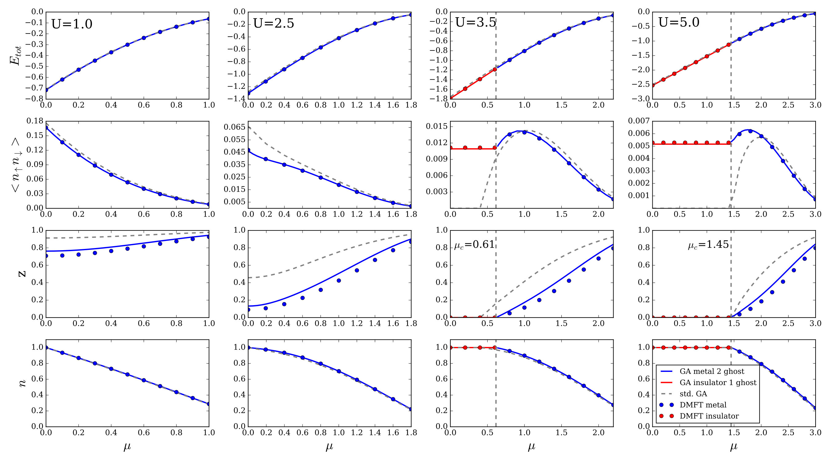 Figure 1
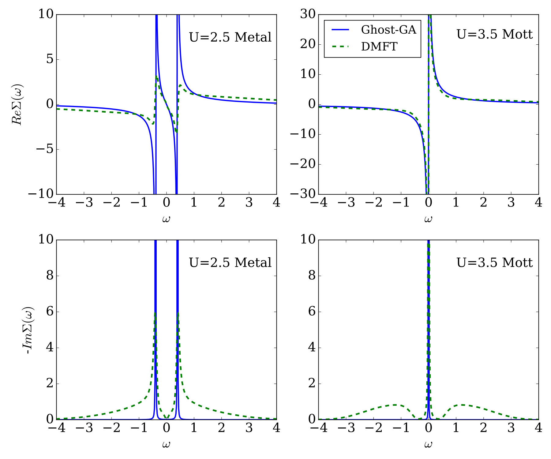 Figure 2
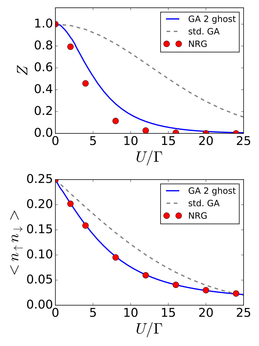 Figure 3
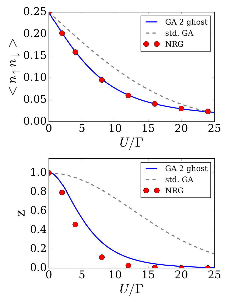 Figure 4
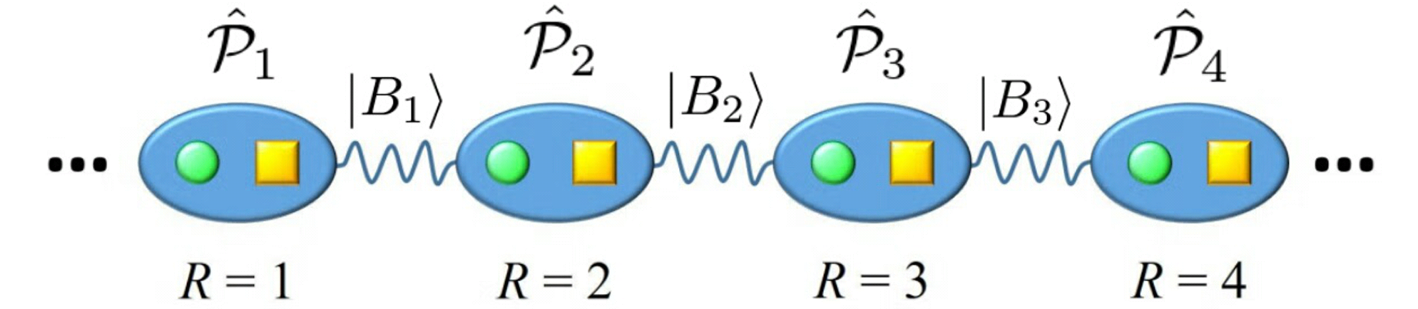 Figure 5
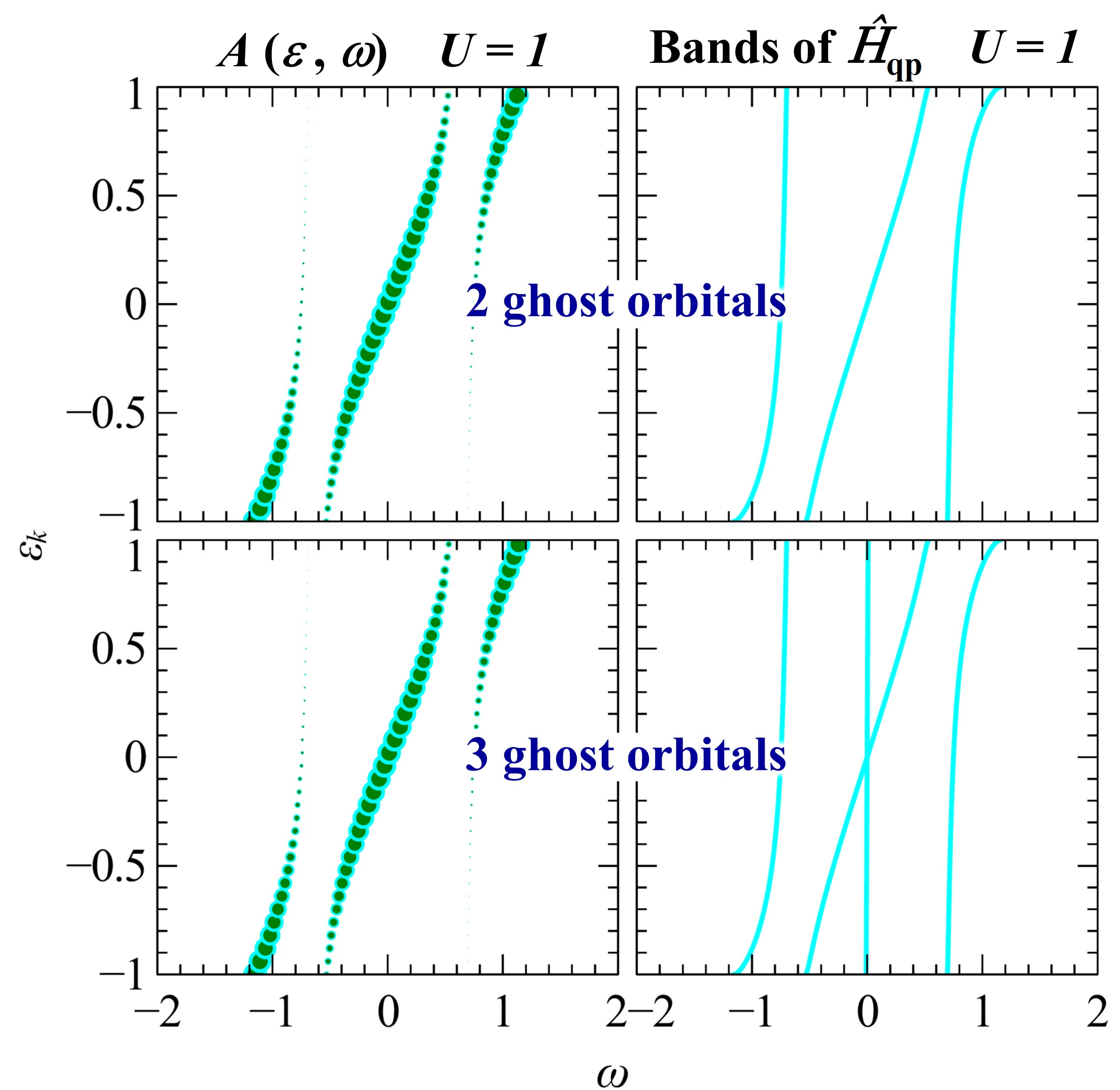 Figure 6
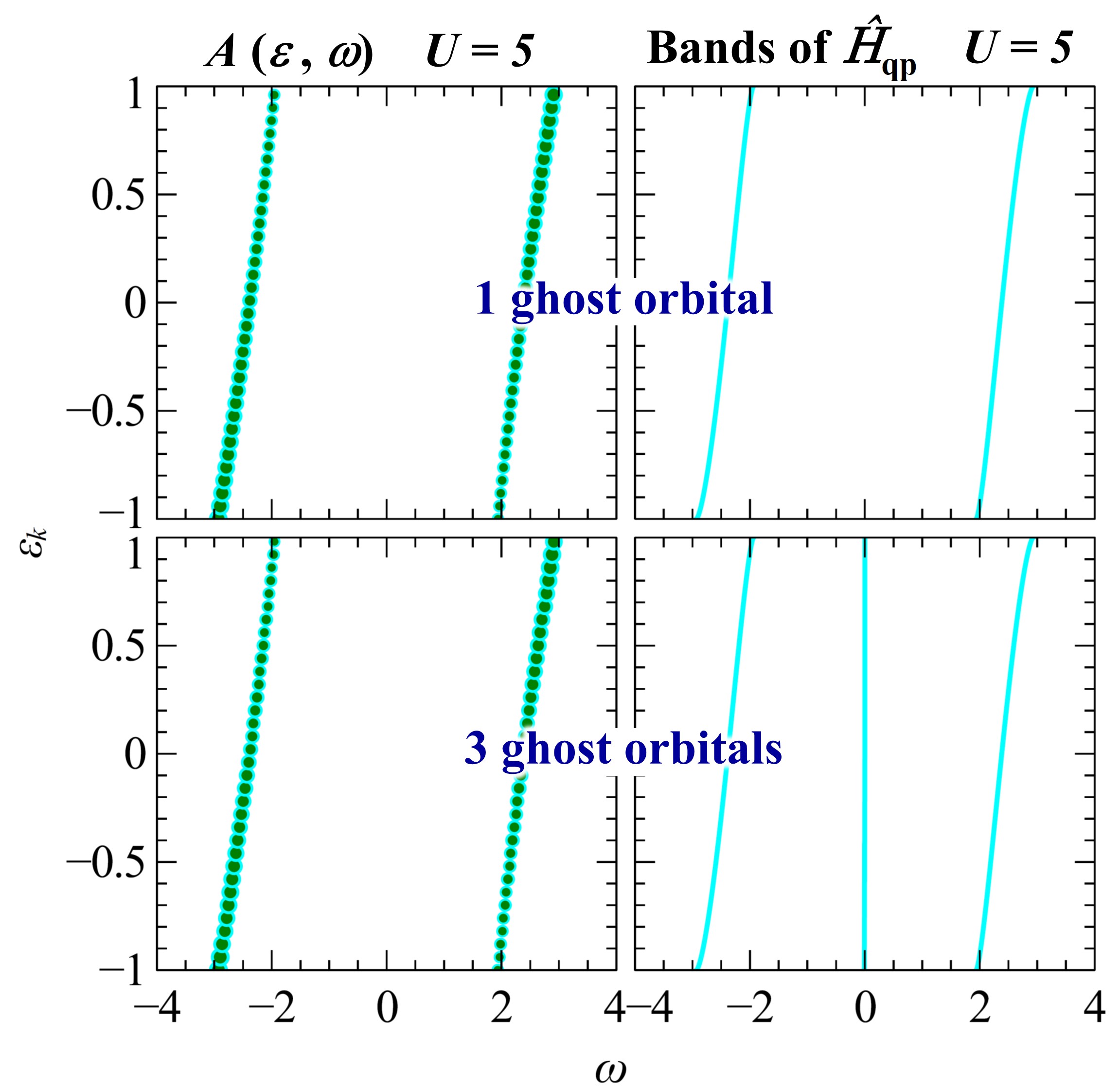 Figure 7
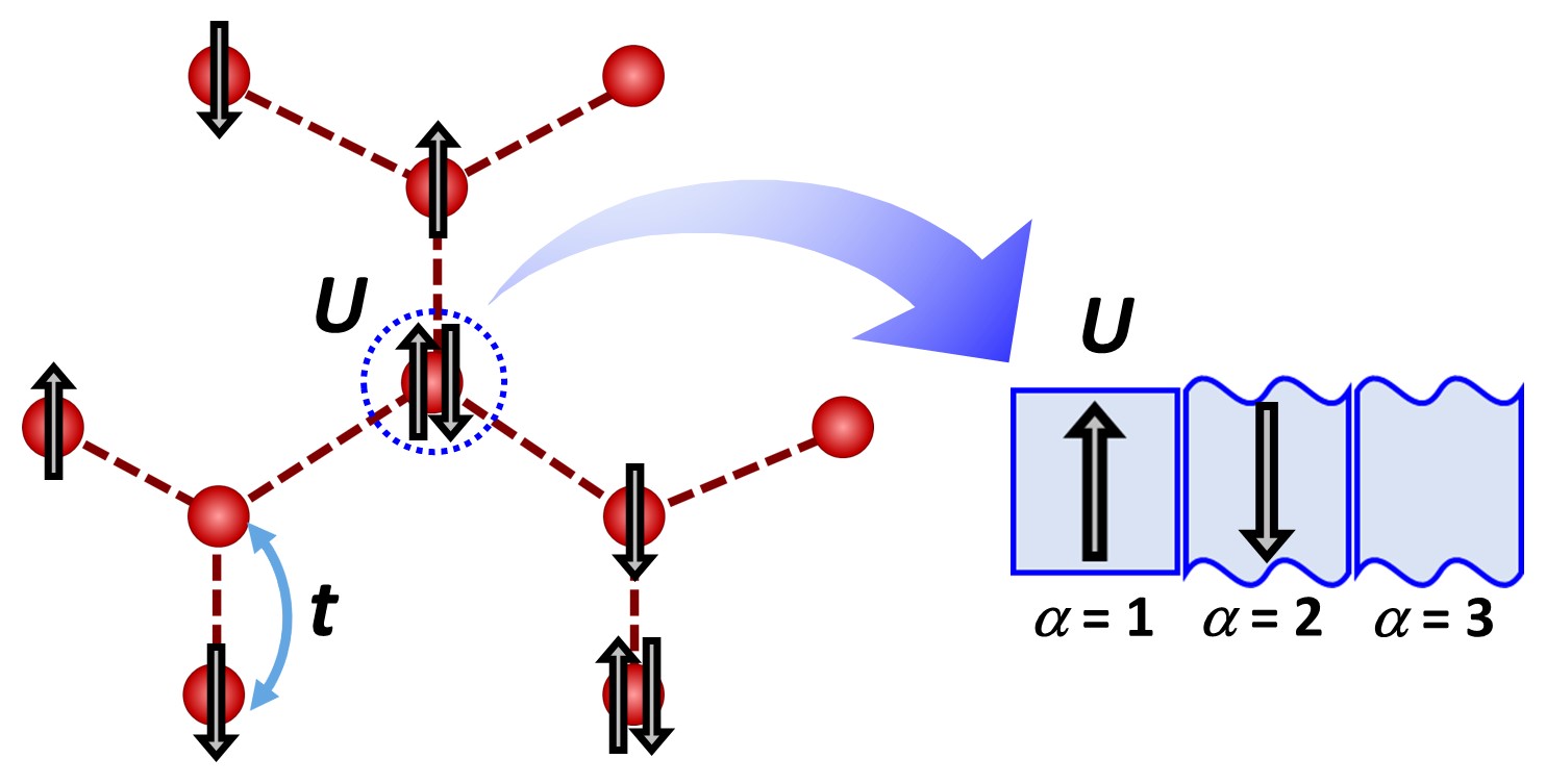 Figure 1
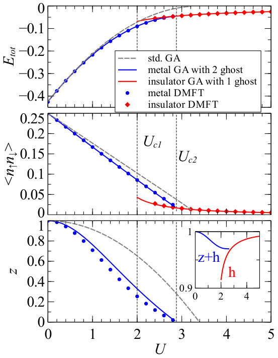 Figure 2
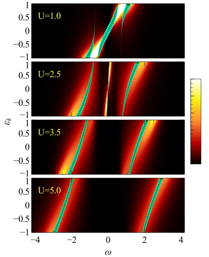 Figure 3
Peer Reviews
No public reviews on file for this paper yet. If you reviewed it on a platform where reviews are public (OpenReview, ICLR, NeurIPS, ICML), you can paste yours below so the community can read it here.
Videos
No videos yet. Explain this paper in a talk, walkthrough, or lecture? Add one.
Emergent Bloch Excitations in Mott Matter
Nicola Lanatà
Department of Physics and National High Magnetic Field Laboratory, Florida State University, Tallahassee, Florida 32306, USA
Tsung-Han Lee
Department of Physics and National High Magnetic Field Laboratory, Florida State University, Tallahassee, Florida 32306, USA
Yong-Xin Yao
Ames Laboratory-U.S. DOE and Department of Physics and Astronomy, Iowa State University, Ames, Iowa IA 50011, USA
Vladimir Dobrosavljević
Department of Physics and National High Magnetic Field Laboratory, Florida State University, Tallahassee, Florida 32306, USA
(March 20, 2024)
Abstract
We develop a unified theoretical picture for excitations in Mott systems, portraying both the heavy quasiparticle excitations and the Hubbard bands as features of an emergent Fermi liquid state formed in an extended Hilbert space, which is non-perturbatively connected to the physical system. This observation sheds light on the fact that even the incoherent excitations in strongly correlated matter often display a well defined Bloch character, with pronounced momentum dispersion. Furthermore, it indicates that the Mott point can be viewed as a topological transition, where the number of distinct dispersing bands displays a sudden change at the critical point. Our results, obtained from an appropriate variational principle, display also remarkable quantitative accuracy. This opens an exciting avenue for fast realistic modeling of strongly correlated materials.
pacs:
71.27.+a, 71.30.+h,71.10.Hf
Introduction:— The physical nature of the excited states in strongly interacting quantum systems has long been a subject of much controversy and debate. Deeper understanding was achieved by Landau, more than half a century ago Landau (1957), who realized that in systems of fermions the Pauli principle provides a spectacular simplification. He showed that many properties of Fermi systems can be understood in terms of weakly interacting quasiparticles (QP), allowing a precise and detailed description of strongly correlated matter. Modern experiments provide for even more direct evidence of such QP excitations, for example from using angle-resolved photoemission spectroscopy (ARPES) Damascelli (2004) or scanning-tunneling microscopy (STM) methods Binnig et al. (1982).
The Fermi liquid paradigm, however, describes only the low energy excitations. At higher energies, the physical properties are often dominated by incoherent processes, which do not conform to the Landau picture. The task to provide a simple and robust theoretical description of such incoherent excitations has therefore emerged as a central challenge of contemporary physics. An intriguing apparent paradox is most evident around the Mott point. Here, ARPES and STM experiments provide often clear evidence of additional well-defined high energy excitations (Hubbard bands) which, while being fairly incoherent, still display relatively well defined Bloch character with pronounced momentum dispersion, see, e.g., Ref. Evtushinsky et al. (2017). As a matter of fact, it is often difficult to experimentally even distinguish the Hubbard bands found in Mott insulators from ordinary Bloch bands found at high energy in conventional band insulators. While such behavior can be already numerically reproduced by some modern many-body approximations Georges et al. (1996); Anisimov and Izyumov (2010), a simple conceptual picture for the apparent Bloch character of such high energy charge excitations is not still available. In particular, variational methods such as the Gutzwiller Approximation (GA) Gutzwiller (1965) — which are often able to reproduce the numerical results in a much simpler semi-analytical fashion — generally capture only the low-lying QP features on the metallic side, but cannot provide a description of charge excitations around the Mott point and in the insulating regime.
The goal of this Letter is to write an appropriate variational wave function able to capture both the (low energy) QP bands and the (high energy) Hubbard bands, within the same theoretical framework. A particularly interesting fact emerging from our theory is that many important features of both types of excitations are encoded in the bare density of states (DOS) of the uncorrelated system and a few renormalization parameters — in a similar fashion as for the QP excitations in Landau theory of Fermi liquids. This is accomplished, similarly as in many other theories for many-body systems, see, e.g., Refs. Affleck et al. (1987); Vaestrate et al. (2008); Schollwock (2011), by enlarging the Hilbert space by introducing auxiliary ”ghost” degrees of freedom. In particular, this construction sheds light on the physical origin of the ”hidden” Bloch character of the Hubbard bands mentioned above. Our calculations of the single-band Hubbard model, which are benchmarked against the Dynamical Mean Field Theory (DMFT) Georges et al. (1996); Anisimov and Izyumov (2010) solution, show that the new wave function quantitatively captures not only the dispersion of the QP but also the Hubbard bands. Furthermore, our theory enables us to describe the Mott transition and the coexistence region between the metallic and the Mott-insulator phases.
Ghost GA theory:— For simplicity, our theory will be formulated here for the single-band Hubbard model
[TABLE]
at half-filling. The generalization to arbitrary multi-orbital Hubbard Hamiltonians is straightforward sup .
In order to construct the Ghost-GA theory we are going to embed the physical Hamiltonian of the system [Eq. (1)] within an extended Hilbert space obtained by introducing auxiliary Fermionic ”ghost” degrees of freedom not coupled with the physical orbitals, see Fig. 1.
Let us represent within the extended Hilbert space mentioned above as follows:
[TABLE]
where are the physical hopping parameters, are the eigenvalues of the first term of , and is the spin.
Our theory consists in applying the ordinary multi-orbital GA theory Lanatà et al. (2008); Bünemann et al. (1998); Lanatà et al. (2015a); Attaccalite and Fabrizio (2003); Deng et al. (2009) to Eq (2). In other words, the expectation value of is optimized variationally with respect to a Gutzwiller wave function represented as , where is the most general Slater determinant, , and acts over all of the local degrees of freedom labeled by — including the ghost orbitals . The variational wave function is restricted by the following conditions:
[TABLE]
which are commonly called ”Gutzwiller constraints”. Furthermore, the so called ”Gutzwiller Approximation” Gutzwiller (1965) — which is exact in the limit of infinite dimensions (where DMFT is exact) — is employed. The minimization of the variational energy will be performed by employing the algorithms derived in Ref. Lanatà et al. (2017).
The basis of our theory is that extending the Hilbert space by introducing the ghost orbitals does not affect the physical Hubbard Hamiltonian , as all of its terms involving ghost orbitals are multiplied by [math], see Eq. (2). The advantage of enlarging the Hilbert space arises exclusively from the fact that the corresponding Ghost-GA multi-orbital variational space is substantially more rich with respect to the original GA variational space (where acts only on the physical degrees of freedom) sup . In this respect, our scheme presents analogies, e.g., with the solution of the Affleck, Lieb, Kennedy and Tasak (AKLT) model Affleck et al. (1987) and with the theories of Matrix Product States (MPS) and Projected Entangled Pair States (PEPS) Vaestrate et al. (2008); Schollwock (2011), which are also variational constructions involving virtual entanglement and local maps foo (a). Further technical details about the role of the ghost orbitals are provided in the supplemental material sup .
As shown in previous works, see, e.g., Refs. Lanatà et al. (2015a), the variational energy minimum of is realized by a wave function where is the ground state of a quadratic multi band Hamiltonian represented as
[TABLE]
where are related to by a proper unitary transformation Lanatà et al. (2008); Lanatà et al. (2015a), the matrices and are determined variationally and are the eigenvalues of . The states and where are the eigen-operators of , represent excited states of Bünemann et al. (2003); Lanatà (2009); sup .
The energy-resolved Green’s function of the physical degrees of freedom () can be evaluated in terms of the excitations mentioned above sup and represented as
[TABLE]
where the subscript ”” indicates that we are interested only in the physical component of the Green’s function. We point out that, since Eq. (6) involves a matrix inversion Savrasov et al. (2006, 2005), the Ghost-GA approximation to the physical self-energy is generally a non-linear function sup — while it is linear by construction in the ordinary GA theory. Note also that the poles of coincide with the eigenvalues of , see Eq. (5).
Application to the single-band Hubbard model:— Below we apply our approach to the Hubbard Hamiltonian [Eq. (2)] at half-filling assuming a semicircular DOS foo (b), which corresponds, e.g., to the Bethe lattice in the limit of infinite connectivity, where DMFT is exact Georges et al. (1996). The half-bandwidth will be used as the unit of energy. The extended Ghost-GA scheme will be applied following the procedure of Ref. Lanatà et al. (2017), utilizing up to 2 ghost orbitals.
In Fig. 2 is shown the evolution as a function of the Hubbard interaction strength of the Ghost-GA total energy, the local double occupancy and the QP weight . Our results are shown in comparison with the ordinary GA theory and with DMFT in combination with Numerical Renormalization Group (NRG). In particular, we employed the ”NRG Ljubljana” impurity solver Zitko (2011).
The agreement between Ghost-GA and DMFT is quantitatively remarkable. In particular, the Ghost-GA theory enables us to account for the coexistence region of the Mott and metallic phases, which is not captured by the ordinary GA theory. The values of the boundaries of the coexistence region , are in good agreement with the DMFT results available in the literature García et al. (2004); Werner and Millis (2007); Bulla (1999); Tong et al. (2001), i.e., , . The Ghost-GA value of , which is the actual Mott transition point at , is particularly accurate. The method also gives a reasonable value for the very small energy scale characterizing the coexistence region, which we can estimate as , consistently with both DMFT and experiments Aguiar et al. (2005); Limelette et al. (2003). We point out also that, as shown in the second panel of Fig. 2, the Ghost-GA approach captures the charge fluctuations in the Mott phase, while this is approximated by the simple atomic limit (which has zero double occupancy) within the Brinkman-Rice scenario Brinkman and Rice (1970).
Interestingly, while at least 2 ghost orbitals are necessary to obtain the data illustrated above for the Metallic solution, 1 ghost orbital is sufficient to obtain our results concerning the Mott phase. Increasing further the number of ghost orbitals does not lead to any appreciable difference sup . As we are going to show, this is connected with the fact that the electronic structures of the Mott and the metallic phases are topologically distinct.
Let us now analyze the Ghost-GA single-particle Green’s function , see Eq. (6). In Fig. 3 is shown the Ghost-GA energy-resolved spectral function in comparison with DMFT Karski et al. (2008).
Although the broadening of the bands (scattering rate), is not captured by our approximation (as it is not captured by the ordinary GA), the positions and the weights of the poles of the Ghost-GA spectral function encode most of the DMFT features, not only at low energies (QP excitations), but also at high energies (Hubbard bands). In order to analyze how the spectral properties of the system emerge within the Ghost-GA theory, it is particularly convenient to express the QP Hamiltonian [Eq. (5)] in a gauge where is diagonal foo (c).
In the metallic phase, an explicit Ghost-GA calculation obtained employing 2 ghost orbitals shows that the matrices and are represented as follows:
[TABLE]
where is the Kronecker delta, and , and are real positive numbers determined numerically as in Ref. Lanatà et al. (2017). The corresponding self-energy, see Eq. (6), is foo (d):
[TABLE]
Thus, the variational parameter of Eq. (8) represents the QP weight, whose behavior was displayed in the third panel of Fig. 2. Note that the overall spectral weight , where is the semicircular DOS, is not as in the ordinary GA theory, but it is , which is almost equal to for all values of (see the inset of the third panel in Fig. 2). The additional spectral contribution , which is not present in the ordinary GA approximation, enables the Ghost-GA theory to account for the Hubbard bands.
In the Mott phase, an explicit Ghost-GA calculation obtained employing 1 ghost orbital shows that the matrices and are represented as follows:
[TABLE]
where and are real positive numbers determined numerically as in Ref. Lanatà et al., 2017. Note that (see the inset of the third panel in Fig. 2). The corresponding self-energy, see Eq. (6), is foo (d):
[TABLE]
The pole of the self energy at , which is the source of the Mott gap, is captured by the Ghost-GA theory.
The analysis above clarifies also why, by construction, within the Ghost-GA approximation the self-energy can develop poles, see Eqs. (9) and (12), but can not capture branch-cut singularities on the real axis.
It is important to point out that the Hilbert space extension that we have introduced in this work has been essential in order to capture the effect of the electron correlations on the topology of the excitations — such as the change of the number of bands at the Mott transition (between 3 bands in the metallic phase and 2 bands in the Mott phase). In fact, without extending the Hilbert space, the ordinary GA theory enables only to renormalize and shift the band structure with respect to the uncorrelated limit , without affecting its qualitative topological structure. On the other hand, extending the Hilbert space enables us to relax this constraint, as , see Eq. (6), is variationally allowed to have any number of distinct poles equal or smaller to the corresponding total (physical and ghost) number of orbitals sup . It is for this reasons that only 1 ghost (2 orbitals) is sufficient to describe the Mott phase of the single-band Hubbard model, while at least 2 ghosts (3 orbitals) are necessary in order to describe its metallic phase — whose spectra includes the QP excitations and the 2 Hubbard bands. A remarkable aspect of this construction is that, within the Ghost-GA theory, the information concerning the spectral function — including the Hubbard bands — is entirely encoded in only 3 parameters () in the Metallic phase, and in 2 parameters () in the Mott phase, see Eqs. (7), (8), (10), (11).
Conclusions:— We derived a unified theoretical picture for excitations in Mott systems based on a generalization of the GA, which captures not only the low-energy QP excitations, but also the Hubbard bands. The essential idea consists in extending the Hilbert space of the system by introducing auxiliary ”ghost” orbitals. This construction enables us to express analytically many important features of both types of excitations in terms of the bare DOS of the uncorrelated system and a few renormalization parameters, in a similar fashion as for the QP excitations in Landau theory of Fermi liquids. In particular, this idea provides us with a conceptual picture which assigns naturally a Bloch character to the Hubbard bands even in Mott insulators. In this respect, we note that our theory presents a few suggestive analogies with the interesting (but rather speculative) idea of ”hidden Fermi liquid” previously introduced by P. W. Anderson Anderson (2008) within the context of the BCS wave function (for superconductors) and the Laughlin’s Jastrow wave function (for the Fractional Hall Effect). In fact, they both propose a descriptions of non-Fermi liquid states related to ordinary Fermi liquids residing in unphysical Hilbert spaces, see, e.g., Ref. Jain and Anderson (2009). From the computational perspective, our Ghost-GA theory constitutes a very promising tool for ab-initio calculations in combination with Density Functional Theory (DFT) Hohenberg and Kohn (1964); Kohn and Sham (1965); Deng et al. (2009); Ho et al. (2008); Lanatà et al. (2015a), as it is substantially more accurate with respect to the ordinary GA approximation, without much additional computational cost. In fact, within the numerical scheme described in Refs. Lanatà et al. (2017); Lanatà et al. (2015a), our theory results in solving iteratively a finite impurity model, where the number of bath sites grows linearly with the total number of ghost orbitals sup . Since there exist numerous available techniques enabling to solve efficiently this auxiliary problem, see, e.g., Refs. Wolf et al. (2015); Saberi et al. (2008); Weichselbaum et al. (2009); Lu et al. (2014); Lanatà et al. (2016), this opens an exciting avenue for realistic modeling of many challenging materials, including predictions of ARPES spectra for complex orbitally-selective Mott insulators. Furthermore, since the Ghost-GA theory is based on the multi-orbital GA Lanatà et al. (2017); Lanatà et al. (2015a), it can be straightforwardly generalized to finite temperatures Lanatà et al. (2015b); Sandri et al. (2013); Wang et al. (2010), to non-equilibrium problems Schirò and Fabrizio (2010); Lanatà and Strand (2012), and to calculate linear response functions Fabrizio (2017). For the same reason, the Ghost-GA theory can be also straightforwardly reformulated Bünemann and Gebhard (2007); Lanatà et al. (2008); Lanatà et al. (2015a) in terms of the rotationally invariant slave boson (RISB) theory Lechermann et al. (2007); Li et al. (1989); sup , whose exact operatorial foundation recently derived in Ref. Lanatà et al. (2017) constitutes a starting point to calculate further corrections Dao and Frésard (2017). It would be also interesting to apply the ghost-orbital Hilbert space extension in combination with the Variational Monte Carlo method Ceperley et al. (1977) or the generalization of the GA to finite dimensions of Ref. Münster and Bünemann (2016), which might lead to a more accurate description of strongly correlated electron systems even beyond the DMFT approximation.
Acknowledgements.
N.L., T.H. and V.D. were partially supported by the NSF grant DMR-1410132 and the National High Magnetic Field Laboratory. Y.Y. was supported by the U.S. Department of energy, Office of Science, Basic Energy Sciences, as a part of the Computational Materials Science Program.
1 I. Technical details about Ghost-GA theory
1.1 A. Introduction
Let us consider a generic multi-orbital Hubbard Hamiltonian represented as
[TABLE]
where is the total number of Fermionic degrees of freedom (both spin and orbital), and is a generic local operator (i.e., any operator that can be expressed in terms of operators with fixed label ).
The multi-orbital Gutzwiller Approximation [Gutzwiller, 1965; Lanatà et al., 2008; Bünemann et al., 1998; Lanatà et al., 2015; Attaccalite and Fabrizio, 2003] (GA) consists in minimizing the expectation value of with respect the most general Gutzwiller wave function:
[TABLE]
where is the most general Slater determinant, , and is the most general map acting over all of the local degrees of freedom labeled by . As discussed in Ref. [Lanatà et al., 2015], it is convenient to represent in a ”mixed basis” representation as follows:
[TABLE]
where
[TABLE]
the occupation numbers are the digits of a generic integer in basis , and the ladder operators are related to through a unitary transformation such that
[TABLE]
The variational wave function is restricted by the following conditions:
[TABLE]
which are commonly called ”Gutzwiller constraints”. Furthermore, the ”Gutzwiller Approximation”, which becomes exact in the limit of infinite dimension [Gutzwiller, 1965] — where Dynamical Mean Field Theory (DMFT) is exact [Georges et al., 1996] — is assumed.
As shown in previous works, see, e.g., Refs. [Lanatà et al., 2008, 2016], the accuracy of the Gutzwiller method is improved substantially when the operator (Gutzwiller projector) is allowed to act also beyond the space generated by the correlated degrees of freedom. The main technical idea underlying the Ghost-GA theory presented in this work consists essentially in creating new auxiliary (inert) orbitals with the sole purpose of enriching the variational space without changing its formal structure (i.e., a Gutzwiller-projected Slater determinant). Of course, as the ordinary GA, the Ghost-GA theory exploits the so called ”Gutzwiller Approximation” [Gutzwiller, 1965], which becomes exact in the limit of infinite dimension (where DMFT is exact). Thus, in summary, the Ghost-GA theory consists in an improved variational approximation to DMFT realized by enlarging the ordinary GA variational space.
Further details about the role of the ghost orbitals are provided in the subsections below.
1.2 B. Functional formulation of the Gutzwiller energy minimization
As discussed in the main text, all of our calculations of the single band Hubbard Hamiltonian [see Eq. 1 of the main text] have been performed by applying the ordinary multi-orbital Gutzwiller theory to the same Hamiltonian ”embedded” within the extended Hilbert space obtained by introducing auxiliary ghost orbitals [see Eq. 2 of the main text]. Specifically, we have employed the numerical procedure derived in described in Refs. [Lanatà et al., 2017, 2015], which we summarize below for completeness.
For simplicity, the theory will be formulated here assuming a translationally invariant Gutzwiller solution. As shown in Refs. [Lanatà et al., 2017, 2015], the minimization of the expectation value of a generic multi-orbital Hamiltonian represented as in Eq. (1) with respect to the Gutzwiller wave function can be conveniently formulated in terms of the following Lagrange function:
[TABLE]
where is the total number of points, and are real numbers, , and are Hermitian matrices, and are generic complex matrices. The auxiliary Hamiltonians and , which are called ”quasiparticle Hamiltonian” and ”Embedding Hamiltonian”, respectively, are defined as follows:
[TABLE]
The auxiliary Fermionic Hamiltonian , which was introduced in Ref. [Lanatà et al., 2015], enables us to exploit techniques such as those developed in quantum chemistry in order to tackle the energy minimization problem. The state , see Eq. (9), is the most general many-body state — with electrons — belonging to the auxiliary embedding Hilbert space mentioned above.
1.3 C. Connection between embedding state and Gutzwiller variational parameters
Let us consider the following expansion of the most general state :
[TABLE]
where , and .
For later convenience, it is important to point out that, as shown in Ref. [Lanatà et al., 2015], the matrix with entries is connected with the Gutzwiller variational parameters as follows:
[TABLE]
where is the matrix defining as in Eq. (3), is matrix with entries
[TABLE]
and . Note that, because of Eq. (6), is diagonal.
1.4 D. Gutzwiller Lagrange equations in the standard multi-orbital GA
Following Ref. [Lanatà et al., 2015], in order to take into account the fact that , and are Hermitian matrices we introduce the following parametrizations:
[TABLE]
where the set of matrices is an orthonormal basis of the space of Hermitian matrices with dimension , are the corresponding transposed matrices, and , and are real numbers, while are complex numbers. The above-mentioned orthonormality is defined with respect to the standard scalar product .
It can be readily shown that the saddle-point conditions of , see Eq. (9), with respect to all of its arguments provides the following system of Lagrange equations:
[TABLE]
where the function appearing in Eqs. (19) and (20) is the Fermi function at zero temperature ().
The solution of the equations above can be obtained numerically employing the following procedure [Lanatà et al., 2015]. (I) Given a set of coefficients and , determine the corresponding matrices and using Eqs. (17) and (18), and calculate using Eq. (19). (II) Calculate by inverting Eq. (20). (III) Calculate the coefficients using Eq. (21) and the corresponding matrix using Eq. (16). (IV) Construct the embedding Hamiltonian and compute its ground state , see Eq. (22), within the subspace with electrons. (V) Determine the left members of Eqs. (23) and (24). The equations (23) and (24) are satisfied if and only if the coefficients and proposed at the first of the steps above identify a solution of the GA Lagrange function. The steps above enable us to reduce the solution of the GA Lagrange equations to a root problem, which can be formally represented as
[TABLE]
that can be readily solved numerically, e.g., using the quasi-Newton method.
All of the expectation values with respect to the Gutzwiller wavefunction can be readily expressed in terms of the states and obtained after convergence.
1.5 E. Proof that the solution of the Ghost-GA equations is disentangled
from the auxiliary ghost subsystem
As explained in the main text, the Ghost-GA theory is formulated by embedding the Hamiltonian within an extended Hilbert space, which includes also auxiliary (ghost) Fermionic degrees of freedom. Such a procedure is obviously licit, as the inequality underlying the variational principle, i.e.,
[TABLE]
where is the ground state energy of , remains valid even if is a generic state of the extended Hilbert space.
Since lives only within the physical subsystem, we already know a-priori that the exact ground state (which realizes the above variational minimum) has to be disentangled from the auxiliary degrees of freedom. Here we demonstrate that, indeed, this condition is satisfied exactly by our converged Ghost-GA solution .
Let us assume that among the Fermionic degrees of freedom in , see Eq. (1), only are physical, while the other degrees of freedom are ghost modes. In other words, is constructed utilizing only the physical ladder operators (which implies, in particular, that ).
It is convenient to represent the Gutzwiller local maps as follows:
[TABLE]
where
[TABLE]
As we are going to show, since depends only on the physical degrees of freedom, i.e., it is constructed utilizing only the physical operators , the coefficients defining the Gutzwiller projector are of the form:
[TABLE]
Consequently, the converged Ghost-GA solution can be represented as
[TABLE]
where , which resides entirely within the physical subsystem, and , which resides entirely within the ghost subsystem, are disentangled.
Let us now demonstrate Eq. (29). Since we assumed that , from Eq. (20) it follows that
[TABLE]
Consequently, the ground state of , see Eq. (11), is such that the subsystem generated by the ghost degrees of freedom is disentangled from the rest of the embedding system. Thus, from Eq. (12) it follows that the matrix can be represented as
[TABLE]
The proof of Eq. (29) (and, in turn, of Eq. (30)) follows immediately from Eqs. (32) and (13).
In summary, we have shown that the Ghost-GA solution, see Eq. (2), does not have any spurious entanglement with the auxiliary ghost degrees of freedom (as expected).
1.6 F. Exploiting Eq. (30) numerically
Since we know a-priori that Eq. (30) must be satisfied by the converged result, it is computationally convenient to impose from the onset this condition onto the Ghost-GA variational parameters.
- •
The first simplification due to Eq. (30) arises from the fact that from Eq. (31) implies that
[TABLE]
Consequently, from Eq. (23) it follows that
[TABLE]
This equation enables us to reduce substantially the computational complexity of the root problem [Eq. (25)], as the dimension of the space of matrices satisfying Eq. (34) has only dimension instead of , see Eq. (18).
- •
The second simplification arises from the fact that, because of Eq. (31), the embedding Hamiltonian [Eq. (11)] is such that its subsystem generated by is disentangled from the ghost degrees of freedom . Consequently, it can be solved independently.
These observations reduce exponentially the scaling of the computational complexity of the problem as a function of the number of ghost orbitals used in the calculation.
1.7 G. Similarities with theory of Matrix Product States (MPS) and
Projected Entangled Pair States (PEPS)
In the previous subsections we have shown that the Ghost-GA wavefunction is disentangled from the auxiliary subsystem. However, as we pointed out in the main text, resides within the entire Hilbert space — including the ghost degrees of freedom. In other words, the Gutzwiller operator maps — which is entangled with the auxiliary subsystem — into the a disentangled state represented as in Eq. (30). It is interesting to note that, in this respect, the Ghost-GA variational framework is very similar to the theory of Matrix Product States (MPS) and Projected Entangled Pair States (PEPS) [Verstraete et al., 2004; Schollwock, 2011].
As we are going to show, the main differences between the Ghost-GA theory and MPS/PEPS are the following:
- •
Within the Ghost-GA theory, the local maps (i.e., the Gutzwiller projectors ) act on a generic ”virtual” Slater determinant belonging to an extended Hilbert space, which is determined variationally.
- •
Instead, MPS/PEPS are variational techniques formulated by applying local maps to fixed ”pair states”, which are also constructed within an extended Hilbert space [Verstraete et al., 2004].
In this respect, the variational ansatz represented in Eq. (2) constitutes an extension of the MPS/PEPS variational space. Of course, as we pointed out above and in the main text, in our work we have also assumed the Gutzwiller Approximation [Gutzwiller, 1965] (which is exact only in the limit of infinite dimensions) and the Gutziller constraints, see Eq. (8) — which are approximations not employed in MPS/PEPS theory. Because of this reason, while our approach constitutes a variationally improved scheme with respect to the ordinary GA, it is not ”numerically exact”.
In order to illustrate more clearly the connection between the Ghost-GA theory and MPS/PEPS, let us consider a generic 1-dimensional Fermionic system belonging to a Hilbert space represented as , where each local subsystem is generated by a set of Fermionic operators , where . In this subsection we are going to assume also that is even. Following, e.g., Ref. [Verstraete et al., 2004], let us consider the following state:
[TABLE]
which is a tensor product of maximally entangled ”bonds” represented as
[TABLE]
where . Note that the state defined in Eq. (35) is a Slater determinant.
Let us now assume that only of the degrees of freedom are physical, i.e., that we are interested in the ground state of a Hamiltonian constructed only with the operators , which are connected to the operators by unitary transformations
[TABLE]
As in Sec. I E, in order to construct a variational approximation of the ground state of , we apply on a Gutzwiller operator , see Fig. 1, where is the most general map acting over all of the local degrees of freedom labeled by represented as follows:
[TABLE]
where
[TABLE]
and the coefficients defining the Gutzwiller projector are of the form:
[TABLE]
Following Ref. [Verstraete et al., 2004], it can be readily verified by inspection that the so obtained state can be represented as follows:
[TABLE]
where is a MPS with bond dimension , which resides entirely within the physical subsystem.
In particular, the observation above clarifies that, within the Ghost-GA variational ansatz, increasing the number of ghost orbitals amounts essentially to increase the so-called ”bond dimension” [Verstraete et al., 2004], which is the parameter controlling the accuracy of the variational ansatz also in MPS/PEPS. However, we remark that within the Ghost-GA theory the state is variationally determined, i.e., it is not restricted to the form [Eq. (36)]. In future works, it would be interesting to apply the ghost-orbital Hilbert space extension without employing the Gutzwiller constraints and the Gutzwiller approximations, e.g., utilizing the Variational Monte Carlo method [Ceperley et al., 1977].
2 II. Ghost-GA excitations from variational parameters
2.1 A. Gutzwiller excitations and ARPES spectra in the standard multi-orbital GA
Let us assume that the Gutzwiller energy minimum is realized by a solution of Eqs. (19)-(24) identified by the variational parameters . Thus, is the ground state of corresponding to the parameters , see Eq. (10). Such a solution corresponds to a Gutzwiller wavefunction which can be represented as
[TABLE]
see Eq. (2). It is important to observe that, in the thermodynamical limit , Eqs. (19)-(24) are satisfied also by , where is any eigenoperator of , see Eq. (10), and is the corresponding eigenvalue. Each one of the corresponding Gutzwiller states can be represented as
[TABLE]
Similarly, Eqs. (19)-(24) are satisfied also by , which correspond to Gutzwiller states represented as
[TABLE]
Since the states [Eqs. (43) and (44)] correspond to saddle points of the Gutzwiller energy functional, they can be interpreted as variational approximations to many-body excitations of the system (with a number of particles differing by 1 with respect to the ground state). It is important to note that each one of these states is connected to a single-particle excitation of through the action of the many-body operator . Thus, these states represent complex collective excitations of the system, which are commonly called ”Gutzwiller-Landau quasiparticles” [Bünemann et al., 2003].
As pointed out in previous publications, see, e.g., Ref. [Lanatà, 2009] and the references therein, this information allows us to evaluate the Gutzwiller ARPES spectra, which is defined as follows:
[TABLE]
The main idea in order to evaluate approximately Eq. (45) consists in inserting projectors over the Gutzwiller-Landau quasiparticle states and (see Eqs. (43) and (44)) in Eq. (45) and use the following identities:
[TABLE]
where are the operators appearing in Eq. (10). From the identities above one can readily obtain [Lanatà, 2009]:
[TABLE]
Note that, in general, [Eqs (44) and (44)] are not a complete basis. In fact, we have that, within the approximations employed in Eq. (48),
[TABLE]
Within the standard GA theory, the interpretation of as the matrix of quasiparticle weights is motivated by the fact that the Green’s function corresponding to Eq. (48) is
[TABLE]
Thus, if is invertible, it can be straightforwardly verified that:
[TABLE]
It is very important to note that Eq. (51), which provides a linear expression for the self-energy as a function of the frequency , is valid only if is invertible. However, we already know that this condition is not satisfied within the Ghost-GA theory, see Eq. (34). This important point will be further stressed in the next subsection.
2.2 B. Gutzwiller excitations and ARPES spectra in the Ghost-GA theory
As explained in the main text and in the previous section of the present supplemental material, the Ghost-GA theory consists in applying the ordinary multi-orbital Gutzwiller theory to the Hamiltonian ”embedded” within the extended Hilbert space obtained by introducing auxiliary ghost orbitals. The only difference with respect to the ordinary theory is that, as shown in the main text, utilizing the enlarged Gutzwiller variational space leads to a better approximation to the ground state and to the excited states and , see Eqs. (43) and (44), which are all saddle points of the Ghost-GA energy functional.
Let us consider again the Hamiltonian , see Eq. (1), embedded within an enlarged Hilbert space. In other words, we assume that is constructed utilizing only the physical ladder operators (which implies, in particular, that ).
The Ghost-GA spectral function of the system is given by the components of the spectral function
[TABLE]
such that . The same steps utilized in the previous section lead to the following approximation to the physical Green’s function:
[TABLE]
Note also that, as expected, from Eqs. (34) and (53) it follows that
[TABLE]
i.e., only the physical components of the Green’s function are non-zero.
The Ghost-GA physical self-energy is given, by definition, by the Dyson equation, i.e., it is the function satisfying the following equation:
[TABLE]
where is given by Eq. (53). It is important to note that, as pointed out above and in the main text, is not invertible, see Eq. (34). Consequently, the Ghost-GA self-energy defined above is not necessarily a linear function of the frequency .
Remarkably, Eq. (55) provides us with an analytical expression for the Ghost-GA spectral function in terms of the bare physical dispersion and a few renormalization parameters, i.e., the matrices and . Of course, the entries of and depend on the specific system considered, as they have to be calculated numerically from Eqs (19)-(24). In particular, Eqs. 8-13 of the main text have been obtained from Eq. (55).
Note that, within the context of the Ghost-GA theory, the excited states and are constructed by applying the Gutzwiller projector to states belonging to the extended Hilbert space. In this respect, these mathematical form of these states present suggestive formal analogies with the ”hidden Fermi liquid” excitations previously introduced by P. W. Anderson [Anderson, 2008; Jain and Anderson, 2009].
We point out also that the construction above is not specific to the single band Hubbard Hamiltonian considered in this work, as it can be straightforwardly applied to generic Hubbard Hamiltonian — with an arbitrary number of physical orbitals.
3 III. Additional Remarks about the benchmark calculations of the single band Hubbard model
3.1 A. Behavior of the Ghost-GA self-energy
As discussed in the main text, the Ghost-GA self-energy of the single band Hubbard Hamiltonian can be represented as follows in the metallic phase:
[TABLE]
while it can be represented as follows in the Mott phase:
[TABLE]
The values of the parameters and evolve as illustrated in Fig. 2 of the main text. The behavior of the Ghost-GA self-energy is shown in Fig. 2 in comparison with DMFT.
As discussed in the main text, some of the main features of the self energy are captured by Eqs. (56) and (57). The differences with respect to the DMFT solution arise mostly from the fact that within the Ghost-GA theory, by construction, the self-energy can develop only poles, see Eqs. (56) and (57), but can not capture branch-cut singularities on the real axis. In other words, the so-called ”scattering rate” is not captured by our approximation (as it is not captured by the ordinary GA).
It is interesting to observe that in the limit of we have and . Thus, from Eq. (56) we deduce that , i.e., the uncorrelated limit is described exactly by our theory. Note that this result is to be expected as, by construction, the Ghost-GA variational space includes all of the Slater determinants.
3.2 B. Ghost-GA solution utilizing 3 ghost orbitals
In this work, the accuracy of the Ghost-GA theory has been explicitly demonstrated (in all regimes of interaction strength) on the single-band Hubbard Model for a semi-circular density of states (DOS) — which corresponds, e.g., to the Bethe lattice in the limit of infinite coordination number, where DMFT is exact. Specifically, the calculations discussed in the main text were performed using 2 ghost orbitals in the metallic phase and 1 ghost orbital in the Mott phase, as this was the minimal ghost extension enabling us to capture the main features of the ARPES spectra and of the phase diagram of the system. In this section we are going to discuss how the Ghost-GA result depends on the number of ghost orbitals used in the calculations.
The Ghost-GA physical Green’s function of the single-band Hubbard model
[TABLE]
see the third member of Eq. (53), is analytical by construction everywhere over the upper-half plane, and has poles over the eigenvalues of:
[TABLE]
However, the physical spectral weights of these poles is generally not because of the presence of the renormalization coefficients in Eq. (58).
As mentioned in the main text, if 2 ghost orbitals are used to study the Mott phase of the Hubbard model, all of the results, including both the ground state properties and the ARPES spectra, remain essentially unchanged. In particular, even though has 3 bands (by construction), the converged values of the renormalization parameters are such that one of these bands is flat and acquires spectral weight [math] (i.e., it does not contribute to the ARPES spectra), while the other 2 bands do not display any visible difference with respect to those computed using only 1 ghost orbital. Here we show that, as expected, the same mechanism occurs when 3 ghost orbitals are used to describe the system, both in the metallic and in the insulating phases of the single-band Hubbard model with semicircular DOS at half-filling.
In Figs. 4 and 4 the Ghost-GA energy-resolved spectral function , see Eq. (58) is analyzed for 2 values of in comparison with the Ghost-GA quasiparticle spectral function \mathrm{Tr}\big{[}\delta(\omega-[\tilde{\mathcal{R}}\,\tilde{\epsilon}\,\tilde{\mathcal{R}}^{\dagger}+\tilde{\lambda}])\big{]}=\sum_{n}\delta(\omega-\tilde{\epsilon}^{*}_{n}), see Eq. (59). The Ghost-GA results obtained in the main text — utilizing 2 ghost orbitals in the metallic phase and 1 ghost orbital in the Mott phase — are compared with the results obtained using 3 ghost orbitals for both phases.
This analysis shows that, in all cases analyzed so far, increasing the number of orbitals (ghost plus physical) beyond the minimal number necessary in order to match the number of bands in the system does not affect the physical spectral function . In particular, in the results shown in Figs. 4 and 4 we observe that the physical spectral function obtained with 3 ghost orbitals displays 1 flat band with zero spectral weight in the metallic phase, while it displays 2 degenerate flat bands with 0 spectral weight in the Mott phase.
3.3 C. Benchmark calculations of the single-band Hubbard model away from half-filling
In order to study the Hubbard Hamiltonian away from half filling, here we work in the grand-canonical ensemble, i.e., we study the following Hamiltonian:
[TABLE]
Note that Eq. (60) is represented in such a way that the particle-hole symmetric case (half-filling) corresponds to .
In Fig. 5 is shown the evolution as a function of the chemical potential of the total energy, the local double occupancy, the QP weight and the local occupancy, for 2 values of the Hubbard interaction strength . The Ghost-GA results are shown in comparison with the ordinary GA theory and with DMFT.
As in the case of half filling considered above and in the main text, the agreement between Ghost-GA and DMFT is quantitatively remarkable.
4 IV. Ghost-GA benchmark calculations of the Single-orbital Anderson Impurity Model
In order to provide further evidence of the quality the Ghost-GA theory and, in turn, to further validate the results provided in the main text, in this section we provide also benchmark calculations of the single-band Anderson Impurity Model (AIM).
[TABLE]
where is the spin label. In particular, we are going to consider the case of a flat density of states, whose hybridization function [Hewson, 1997] can be represented as follows:
[TABLE]
where is the Heaviside step function.
In Fig. 6 is shown the evolution as a function of the Hubbard interaction strength of the impurity double occupancy and the QP weight . The Ghost-GA results obtained by adding 2 ghost orbitals on the impurity site are shown in comparison with the ordinary GA theory and with NRG.
Consistently with the benchmark calculations of the Hubbard model considered above and in the main text, here we observe that the accuracy of the Ghost-GA solution is quantitatively remarkable also for the AIM. In particular, we note that the Ghost-GA results are substantially more accurate with respect to the ordinary GA — as expected, since the Ghost-GA theory enlarges the ordinary Gutzwiller variational space.
It is interesting to analyze more in detail the behavior of (which is commensurate with the Kondo temperature [Hewson, 1997]), in the strong-coupling regime . It is well known that the ordinary Gutzwiller theory provides, even without ghost orbitals, an exponentially decaying Kondo scale in the large- limit: . The only well-known discrepancy of this result with respect to the exact solution of the AIM is that the Gutzwiller prefactor at the exponent is , while the exact universal numerical value is , see, e.g., Eqs. 101-102 of Ref. [Lanatà, 2010] and the references therein. A numerical analysis of the results displayed in Fig. 6 shows that the Ghost-GA theory obtained by adding 2 ghost orbitals provides, in particular, a more accurate estimation of the universal prefactor in front of at the exponent of the expression for , which behaves as in the large- regime.
A more detailed study of the AIM will be provided in future publications.
5 V. Ghost Rotationally Invariant Slave Boson (Ghost-RISB) theory
As mentioned in the conclusions of the main text, the Ghost-GA theory can be equivalently reformulated as the mean field approximation of an alternative formulation of the Rotationally Invariant Slave Boson (RISB) theory, which we call Ghost-RISB theory. For completeness, this construction is briefly described in this section.
Let us consider a generic Hubbard Hamiltonian represented as in Eq. (1). In Ref. [Lanatà et al., 2017] it was demonstrated that Eq. (1) can be equivalently reformulated as a gauge theory in an auxiliary Hilbert space (i.e., the RISB theory), and that this exact reformulation of the many-body problem reduces to the ordinary GA at the mean-field level.
Here we observe that the mapping mentioned above could be equivalently applied to the Hubbard Hamiltonian expressed within a Ghost-GA extended Hilbert space. Of course, this construction would result in an alternative exact reformulation of the many body problem, which we call Ghost-RISB theory. However, by construction, the Ghost-RISB theory reduces to the Ghost-GA theory at the mean field level — which is substantially more accurate with respect to the ordinary GA. Because of this reason, it would be very interesting to explore the possibility of taking into account fluctuations beyond mean-field within the framework of the Ghost-RISB, as it has been done in previous works within the ordinary SB theory [Dao and Frésard, 2017].
References
- Gutzwiller (1965)
M. C. Gutzwiller, Phys. Rev. 137, A1726 (1965).
- Lanatà et al. (2008)
N. Lanatà, P. Barone, and M. Fabrizio, Phys. Rev. B 78, 155127 (2008).
- Bünemann et al. (1998)
J. Bünemann, W. Weber, and F. Gebhard, Phys. Rev. B 57, 6896 (1998).
- Lanatà et al. (2015)
N. Lanatà, Y. Yao, C.-Z. Wang, K.-M. Ho, and G. Kotliar, Phys. Rev. X 5, 011008 (2015).
- Attaccalite and Fabrizio (2003)
C. Attaccalite and M. Fabrizio, Phys. Rev. B 68, 155117 (2003).
- Georges et al. (1996)
A. Georges, G. Kotliar, W. Krauth, and M. J. Rozenberg, Rev. Mod. Phys. 68, 13 (1996).
- Lanatà et al. (2016)
N. Lanatà, Y.-X. Yao, X. Deng, C.-Z. Wang, K.-M. Ho, and G. Kotliar, Phys. Rev. B 93, 045103 (2016).
- Lanatà et al. (2017)
N. Lanatà, Y. Yao, X. Deng, V. Dobrosavljević, and G. Kotliar, Phys. Rev. Lett. 118, 126401 (2017).
- Verstraete et al. (2004)
F. Verstraete, D. Porras, and J. I. Cirac, Phys. Rev. Lett. 93, 227205 (2004).
- Schollwock (2011)
U. Schollwock, Annals of Physics 96, 326 (2011).
- Ceperley et al. (1977)
D. Ceperley, G. V. Chester, and M. H. Kalos, Phys. Rev. B 16, 3081 (1977).
- Bünemann et al. (2003)
J. Bünemann, F. Gebhard, and R. Thul, Phys. Rev. B 67, 075103 (2003).
- Lanatà (2009)
N. Lanatà, Ph.D. thesis, SISSA-Trieste (2009).
- Anderson (2008)
P. W. Anderson, Phys. Rev. B 78, 174505 (2008).
- Jain and Anderson (2009)
J. K. Jain and P. W. Anderson, Proc. Nat. Acad. Sci. 106, 9131 (2009).
- Hewson (1997)
A. C. Hewson, The Kondo Problem to Heavy Fermions (Cambridge University Press, 1997).
- Lanatà (2010)
N. Lanatà, Phys. Rev. B 82, 195326 (2010).
- Dao and Frésard (2017)
V. H. Dao and R. Frésard (2017), eprint cond-mat/1702.00228.
The reference list from the paper itself. Each links out to its DOI / PubMed record.
- 1Landau (1957) L. D. Landau, Soviet Physics JETP 3 , 920 (1957).
- 2Damascelli (2004) A. Damascelli, Physica Scripta T 109 , 61 (2004).
- 3Binnig et al. (1982) G. Binnig, H. Rohrer, C. Gerber, and E. Weibel, Phys. Rev. Lett. 49 , 57 (1982).
- 4Evtushinsky et al. (2017) D. V. Evtushinsky, M. Aichhorn, Y. Sassa, Z.-H. Liu, J. Maletz, T. Wolf, A. N. Yaresko, S. Biermann, S. V. Borisenko, and B. Buchner (2017), eprint cond-mat/1612.02313.
- 5Georges et al. (1996) A. Georges, G. Kotliar, W. Krauth, and M. J. Rozenberg, Rev. Mod. Phys. 68 , 13 (1996).
- 6Anisimov and Izyumov (2010) V. Anisimov and Y. Izyumov, Electronic Structure of Strongly Correlated Materials (Springer, 2010).
- 7Gutzwiller (1965) M. C. Gutzwiller, Phys. Rev. 137 , A 1726 (1965).
- 8Affleck et al. (1987) I. Affleck, T. Kennedy, E. H. Lieb, and H. Tasaki, Phys. Rev. Lett. 59 , 799 (1987).