A task-driven implementation of a simple numerical solver for hyperbolic conservation laws
Mohamed Essadki (IFPEN, FR3487, EM2C), Jonathan Jung (LMAP), Adam, Larat (FR3487, EM2C), Milan Pelletier (EM2C), Vincent Perrier (LMAP)

TL;DR
This paper presents a task-driven implementation of a simple first-order numerical solver for hyperbolic conservation laws within the StarPU runtime, analyzing efficiency, GPU suitability, and potential for higher-order methods.
Contribution
It introduces a task-based approach for hyperbolic conservation laws and evaluates its performance and scalability on heterogeneous computing systems.
Findings
Task distribution is efficient with numerous large tasks.
GPU acceleration benefits are limited to suitable tasks.
Higher local arithmetic intensity can be achieved with more complex models.
Abstract
This article describes the implementation of an all-in-one numerical procedure within the runtime StarPU. In order to limit the complexity of the method, for the sake of clarity of the presentation of the non-classical task-driven programming environnement, we have limited the numerics to first order in space and time. Results show that the task distribution is efficient if the tasks are numerous and individually large enough so that the task heap can be saturated by tasks which computational time covers the task management overhead. Next, we also see that even though they are mostly faster on graphic cards, not all the tasks are suitable for GPUs, which brings forward the importance of the task scheduler. Finally, we look at a more realistic system of conservation laws with an expensive source term, what allows us to conclude and open on future works involving higher local arithmetic…
Click any figure to enlarge with its caption.
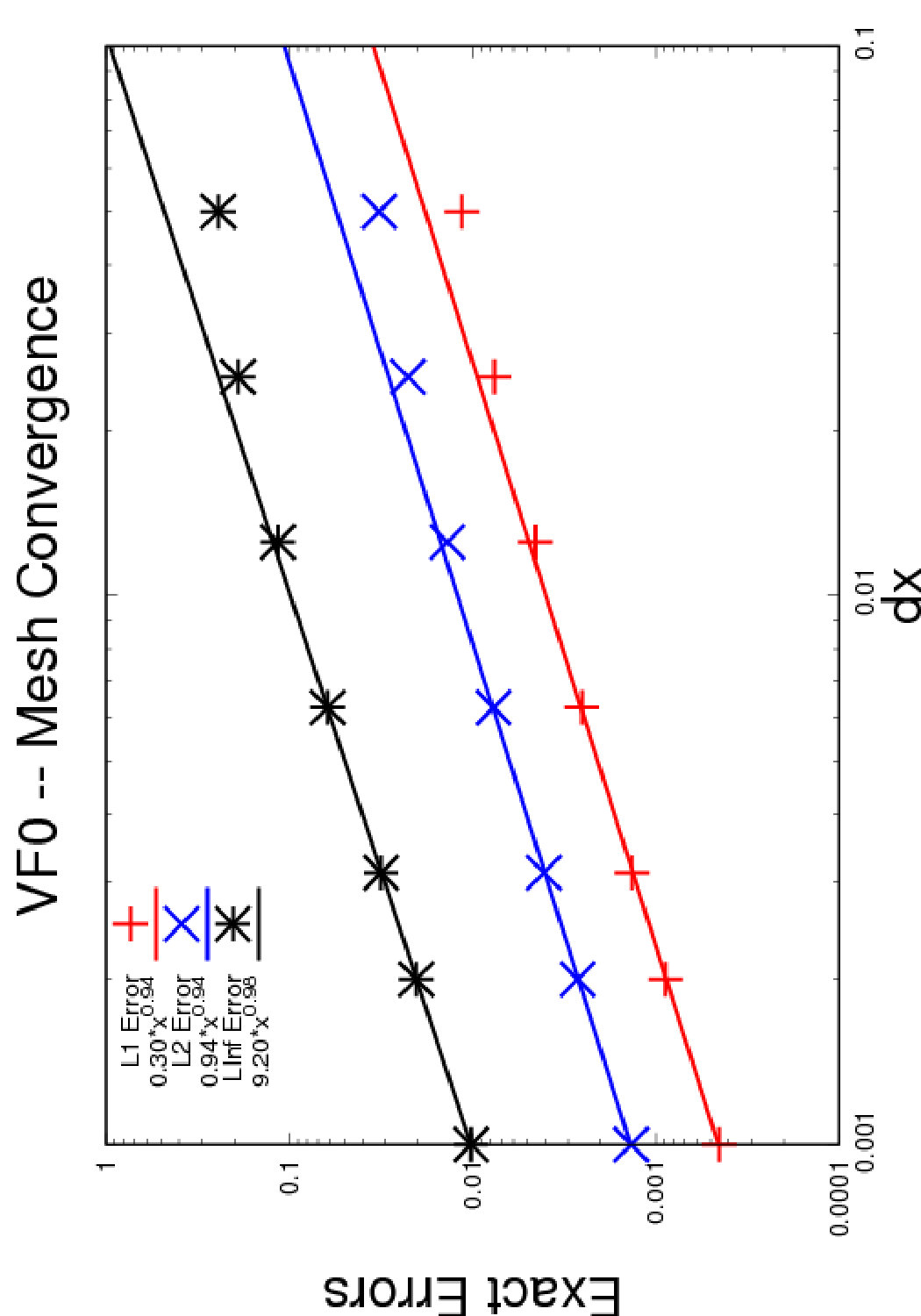 Figure 1
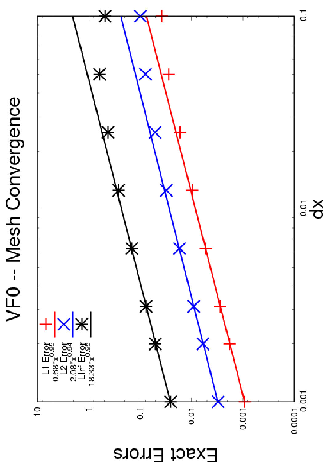 Figure 2
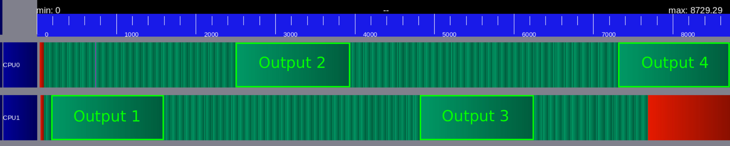 Figure 3
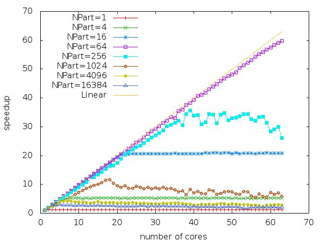 Figure 4
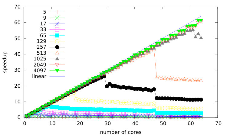 Figure 5
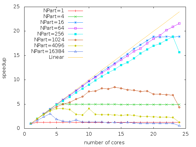 Figure 6
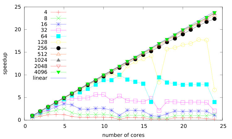 Figure 7
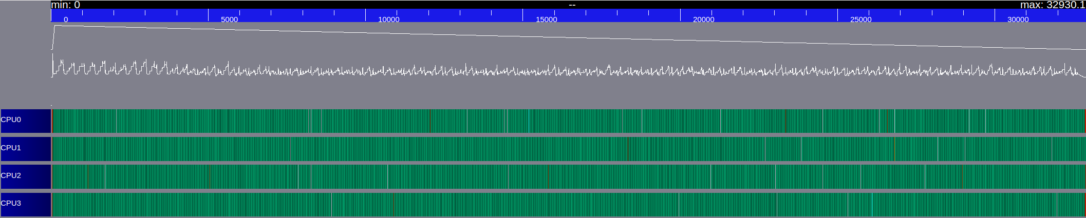 Figure 8
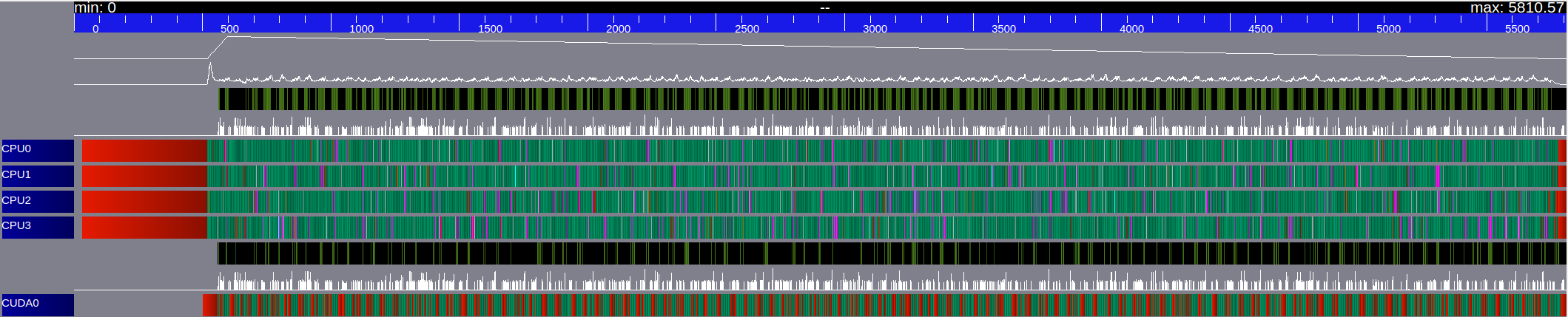 Figure 9
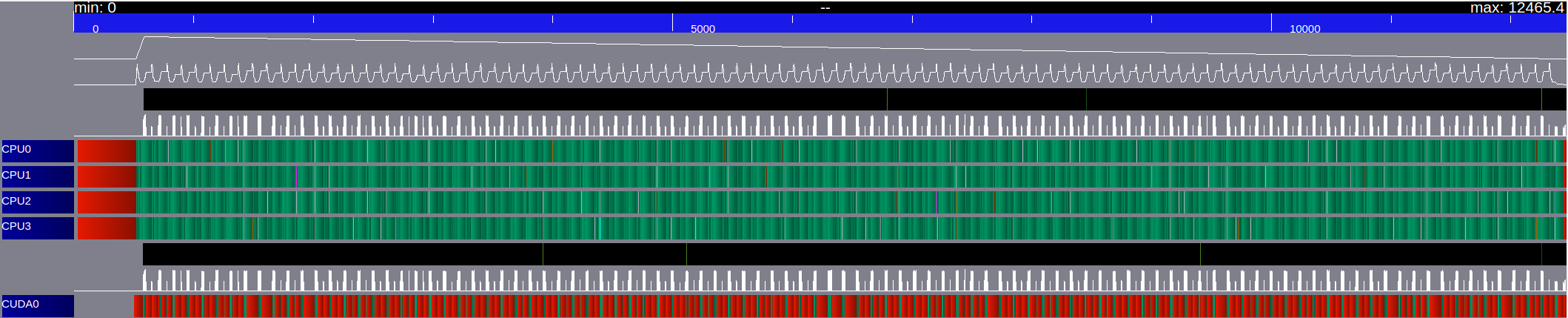 Figure 10
 Figure 11
 Figure 12
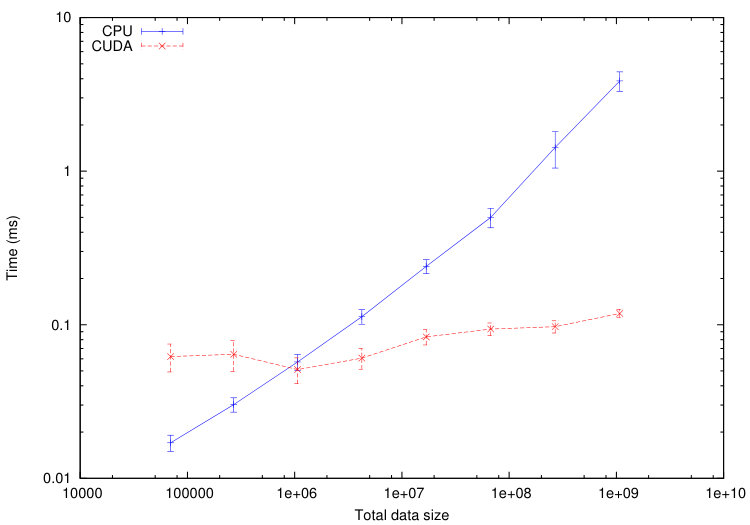 Figure 13
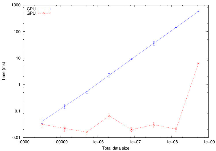 Figure 14
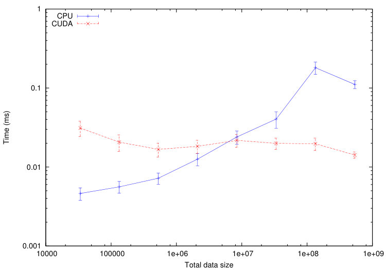 Figure 15
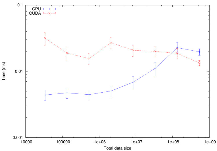 Figure 16
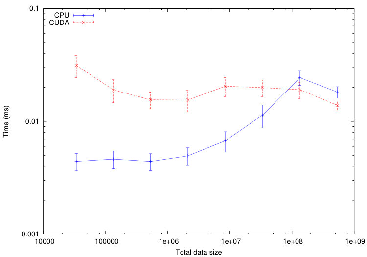 Figure 17
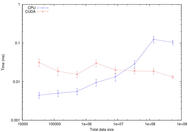 Figure 18
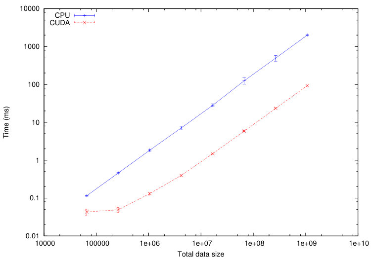 Figure 19
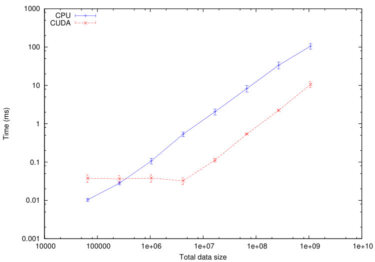 Figure 20
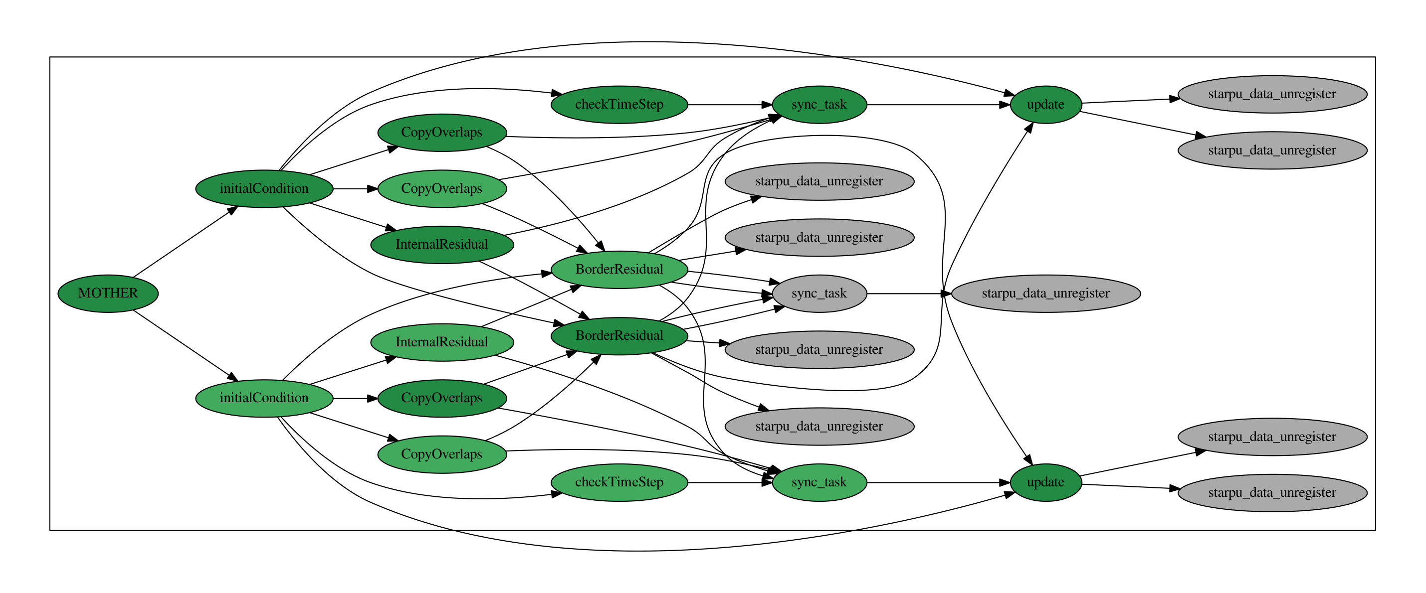 Figure 21
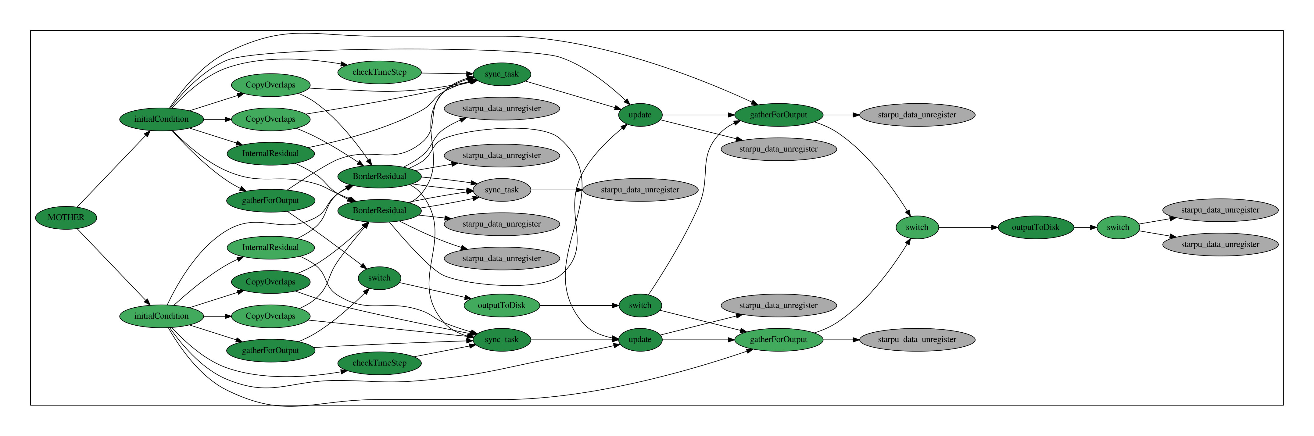 Figure 22
| scheduler | part. | 0 GPU | 1 GPU |
|---|---|---|---|
| eager | 36.06 | 33.12 | |
| 36.40 | 12.42 | ||
| 37.26 | 10.26 | ||
| 38.87 | 15.37 | ||
| dmda | 69.61 | 13.76 | |
| 44.76 | 11.46 | ||
| 39.33 | 10.94 | ||
| 39.31 | 12.98 |
Peer Reviews
No public reviews on file for this paper yet. If you reviewed it on a platform where reviews are public (OpenReview, ICLR, NeurIPS, ICML), you can paste yours below so the community can read it here.
Videos
No videos yet. Explain this paper in a talk, walkthrough, or lecture? Add one.
Taxonomy
TopicsParallel Computing and Optimization Techniques · Distributed and Parallel Computing Systems · Lattice Boltzmann Simulation Studies
\secondaddress
IFP Énergies nouvelles, 1-4 avenue de Bois-Préau, 92852 Rueil-Malmaison Cedex - France
\secondaddressCagire Team, INRIA Bordeaux Sud-Ouest, Pau - France
\sameaddress1 \secondaddressFédération de Mathématiques de l’École Centrale Paris, CNRS FR 3487, Grande Voie des Vignes, 92295 Châtenay-Malabry
\sameaddress1
\sameaddress4, 3
A task-driven implementation of a simple numerical solver for hyperbolic conservation laws
Mohamed Essadki
Laboratoire EM2C, CNRS, CentraleSupélec, Université Paris Saclay, Grande Voie des Vignes, 92295 Châtenay-Malabry - France
,
Jonathan Jung
LMAP UMR 5142, UPPA, CNRS
,
Adam Larat
,
Milan Pelletier
and
Vincent Perrier
Abstract.
This article describes the implementation of an all-in-one numerical procedure within the runtime StarPU. In order to limit the complexity of the method, for the sake of clarity of the presentation of the non-classical task-driven programming environnement, we have limited the numerics to first order in space and time. Results show that the task distribution is efficient if the tasks are numerous and individually large enough so that the task heap can be saturated by tasks which computational time covers the task management overhead. Next, we also see that even though they are mostly faster on graphic cards, not all the tasks are suitable for GPUs, which brings forward the importance of the task scheduler. Finally, we look at a more realistic system of conservation laws with an expensive source term, what allows us to conclude and open on future works involving higher local arithmetic intensity, by increasing the order of the numerical method or by enriching the model (increased number of parameters and therefore equations).
{resume}
Dans cet article, il est question de l’implémentation d’une méthode numérique clé-en-main au sein du runtime StarPU. Afin de limiter la complexité de la méthode et ce dans le soucis de clarifier la présentation de notre méthode dans le cadre de la programmation par tâche, nous avons limité l’ordre de la méthode numérique à un en temps et en espace. Les résultats montrent que la distribution de tâches est efficace si les tâches sont suffisamment nombreuses et de taille suffisante pour couvrir le temps supplémentaire de gestion des tâches. Ensuite, nous observons que même si certaines tâches sont nettement plus rapides sur carte graphique, elles ne sont pas toutes éligibles à un portage sur GPU, ce qui met en avant l’importance d’un répartiteur de tâche intelligent. Enfin, nous regardons un système de lois de conservation plus tournée vers l’application, incluant notamment un terme source coûteux en terme de temps de calcul. Ceci nous permet de conclure et d’ouvrir sur un travail futur, dans lequel l’intensité arithmétique locale sera augmentée par le biais d’une méthode numérique ou d’un modèle d’ordres plus élevés.
1. Introduction
Computations of turbulent flows has been undergoing two breakthrough over the last three decades, concerning computational architectures and numerical methods. On the one hand, computing clusters are reaching a size of many hundreds of thousands of cores, which nowadays allows to overcome RANS modeling by considering unstationary LES simulations [2, 5]. On the other hand, this new framework requires high order numerical methods, which have also been much improved recently [2, 11, 3]. Nevertheless, these newly manufactured massively multicore computers rely on heterogeneous architectures. In order to improve the efficiency of our methods on these architectures, their implementation and algorithmic must be redesigned. The aim of this project is to optimize the implementation of all-in-one numerical methods and models on emerging heterogeneous architectures by using runtimes schedulers. In this publication, we focus on StarPU [1].
Runtime schedulers allow to handle heterogeneous architectures in a transparent way. For this, the algorithm must be recast in a graph of tasks. Computing kernels must then be written in different languages, in order to be executed on the different possible devices. Then, the runtime scheduler will be in charge of dynamically balancing the tasks on the different available computing resources (cores of the host, accelerators, etc.).
Finite differences methods have already been successfully ported on hybrid architectures [7]. However, we aim at developping numerics on unstructured meshes, for example of the discontinuous Galerkin type, and our methods have a very different memory access pattern, which is one of the bottlenecks of the task-driven programming. In order to minimize the complexity of our presentation, gathering both the numerical procedure and its implementation within the non-classical StarPU framework, we have decided to restrict its scope to first order in space and time.
2. A first order finite volume solver for two dimensional conservation laws
2.1. Hyperbolic conservation laws
Let be a subset of . We consider a two dimensional system of conservation laws with source terms
[TABLE]
where is the time, with the spatial position, () is the vector of conservative variables, is the flux function and represents the source terms. Later, the number of conserved variables is noted . The unknowns depend on the spatial position and on the time . We assume that system (1) is hyperbolic, meaning that the directional Jacobian is diagonalizable in every direction , and we note its eigenvalues, the direction n being implicit. We aim at computing a solution of (1) with initial condition
[TABLE]
2.2. Finite volume discretization
In this section, we present a simple numerical scheme which solves system (1) in space and time: If Nx and Ny are two given positive integers, we define the sequences and by and , so that is discretized into cells . We also consider a sequence of times such that , which defines the time steps .
2.2.1. Hyperbolic part
Next, for any cell of the mesh, at any time , we look for an approximation of the average value of the solution on the cell:
[TABLE]
By integrating system (1) over a cell , one obtains:
[TABLE]
where is the outward unit normal to the boundary . Then, the first order explicit finite volume scheme writes [8]:
[TABLE]
where is a chosen numerical flux. In all our computations, the first order Lax-Friedrichs flux will be used:
[TABLE]
with
[TABLE]
The numerical scheme (4) is stable provided the following CFL condition is ensured
[TABLE]
In practice, a constant time step is set at start, and therefore we just need to check at the beginning of each iteration that satisfies inequality (5).
2.2.2. Source term
Since we consider only a first order numerical scheme in space and time, the source term treatment can be simply added by use of a first order operator splitting technique [6].
Therefore, the additional source terms can possibly be taken into account by local cell-wise integration of the following ODE, which is simply discretized by mean of a forward Euler time scheme:
[TABLE]
where is the partial update given by the Finite Volume integration (4). Let us note that though the update (6) is simple and cheap, the computation of may be rather complex and computationnally expensive.
3. StarPU: a task scheduler
Task scheduling offers a new approach for the implementation of numerical codes, which is particularly suitable when looking for an execution on heterogeneous architectures.
The structure of the codes is divided into two main layers that we will call here bones and flesh. At first level, the code is parsed to build a tasks dependency graph that can be viewed as its skeleton. Next, one enters within this graph of tasks and starts executing the actions associated to each of these tasks. Then, the code acts on the memory layout thanks to what can be viewed as its muscles. During the execution part, one may have different choices in the tasks execution on the available computational power and this is where the scheduler plays its role: it aims at distributing the actions so as to minimize the global computational time.
Now, we detail the glossary attributed to such a new implementation framework within the context of the StarPU runtime.
3.1. StarPU tasks
In StarPU, a task is made of the following: a codelet, associated kernels and data handles.
- •
The codelet is the task descriptor. It contains numerous information about the task, including the number of data handles, the list of available kernels implemented to execute this task (for CPU, GPU or possibly something else…) and the memory access mode for each data handle: "Read" (R), "Write" (W) or "Read and Write" (RW).
- •
The kernels are the functions that will be executed on a dedicated architecture: CPU, GPU, etc. A task may have the choice between different kernels implementation and it is the role of the StarPU scheduler to distribute the tasks on the available heterogeneous architectures following a certain criterion (in general minimizing the global execution time).
- •
The data handles are the memory managers. Each data handle can be viewed as the encapsulation of a memory allocation, which allows to keep trace of the action (read or/and write) of the task kernel on the memory layout. In particular, this allows to build the task dependency graph.
3.2. Construction of the tasks dependency graph
The domain of size is partitioned into balanced parts of size , see Figure 1. One task will deal with one partition at a time. In order to treat the interaction between the domains in an asynchronous manner, each domain is supplemented with copies of its border data, see Figure 2.
- •
Each memory allocation is associated with a data handle: one for each subdomain, four for its borders copy, called overlaps in the following,
- •
The codelet of each task points toward a certain number of these data handles, tagged as "R" or "W" or "RW", for Read and/or Write, following the access mode exepected by the associated kernel,
- •
Finally, the code is parsed and the tasks are submitted to StarPU. When a task has to write on a certain data handle memory, a dependency edge is drawn between this task and the latest tasks having read access on this data handle. Similarly, for each of its read-accessed data handles, a task will depend on the latest tasks having write access on them.
- •
Once the dependency graph is built, the tasks are distributed in dependency order by the scheduler on the available computational ressources, following the available kernel implementations. Note that building the dependency graph and lauching the task can be an intricated work, especially since the future of the graph may depend on the computation itself: think of the number of time steps which may depend on the solution, for example.
3.3. Task overhead
StarPU tasks management is not free in terms of CPU time. In fact, each task execution presents a latency called "overhead". We want to know when this additional time can be neglected or not. There is a StarPU benchmark that allows to measure the minimal duration of a task to ensure a good scalibility. We send short tasks with the same (short) duration varying between and and we study the scalability. In Figure 3, we plot the results obtained on a 2 dodeca-core Haswell Intel Xeon E5-2680 and on a Xeon Phi KNL with the scheduler eager. On few cores, we have a good scalibility result, even if the duration of the tasks is short (). On many cores, we need longer tasks duration to get satisfying scaling ().
To sum up, if the duration of the tasks is smaller than the microsecond, their overhead cannot be neglected anymore.
3.4. Schedulers
The purpose of the scheduler is to launch the tasks when they become ready to be executed. In StarPU, many different scheduling policies are available. In this paper, we consider only the two following:
- •
the eager scheduler: it is the scheduler by default. It uses a central task queue. As soon as a worker has finished a task, the next task in the queue is submitted to this worker.
- •
the dmda scheduler: this scheduler takes into account the performance models and the data transfer time for the tasks (see Section 5.3.2). It schedules the tasks so as to minimize their completion time by carefully choosing the optimal executing architecture.
4. Practical Implementation
After a general presentation of the model and the numerical method in section 2 and of the runtime environment with a particular focus on StarPU in section 3, we now detail the way we have implemented this numerical resolution of a system of hyperbolic conservation laws within the task-driven framework StarPU.
4.1. Memory allocation
Since the tasks dependency graph is mainly based on the memory dependency between successive tasks, memory allocation is a crucial development part of our application. This starts with the definition of the structure Cell, which contains the conserved variables at a certain point in space and time.
4.1.1. Principal variables
For a first order finite volume resolution of a system of conservation laws, only two main variables are needed:
- •
u, the computed solution. In each mesh cell, it contains floats. However, since at first order , u contains only one Cell structure of size nVar corresponding to one local approximation (3) of the solution per mesh cell.
- •
RHS, the vector of residuals. It has exactly the same memory characteristics as u, since at each time step, the update is done by:
[TABLE]
These two vectors of variables are allocated per subdomain. Typically, for each of the subdomains, a vector uLoc of Cells is created and encapsulated in a StarPU data handler which allows to follow the memory dependency.
4.1.2. Overlap additional memory buffers
In order to minimize the communications and the dependencies between subdomains, each subdomain comes with four additional one-dimensional buffers corresponding to the possible four overlap-data needed at the subdomain boundaries (East, North, West and South).
Two vectors of size (ovlpS and ovlpN) and two vectors of size (ovlpE and ovlpW) are always allocated, whether the overlap needs to be used or not. The reason for that is that the number of data handlers passed to a StarPU kernel needs to be constant. Therefore, when copying the overlap-data for example, all the overlap data handlers are passed anyway but nothing is done if they are not needed, like in the case of a periodic subdomain in one direction.
Of course, here lies a small communication optimization, when sending a task on another device, since some useless data is transfered. However, we think that the overlap tasks should be of negligeable size compared to the task acting on the entire subdomains and should be mainly executed on the host node.
4.2. Description of the tasks
In paragraph 2.2.1, we have seen that the first order finite volume method essentially consists in
- checking the computational time step ,
- computing all the numerical fluxes at all the edges of the mesh,
- gathering them in the RHS vector and finally
- updating the numerical solution u.
Based on this general decomposition, here is the list of tasks implemented in our application. Between brackets is specified the memory data handlers accessed by the task, with their respective access rights given between parentheses:
- •
initialCondition[uLoc(W)]: fills each subdomain solution with the initial condition.
- •
checkTimeStep[uLoc(R)]: computes the largest characteristic speed within the subdomain. In order to avoid gathering these time constraints globally, we only check that the fixed time step initially given by the user respects locally the stability constraint.
- •
copyOverlaps[ovlpE(W),ovlpN(W),ovlpW(W),ovlpS(W),uLoc(R)]: each subdomain fills the corresponding neighbors overlap data vectors, if needed. This is not the case if the subdomain is periodic in one or both directions, or if one of the boundary states is prescribed (Dirichlet boundary condition). The northest (*resp. *southest) line of the subdomain is copied in the ovlpS (*resp. *ovlpN) data handle of the northern (*resp. *southern) neighbor. The extreme east (*resp. *extreme west) column is copied in the ovlpW (*resp. *ovlpE) data handle of the eastern (*resp. *western) neighbor. Figure 4 depicts the copyOverlaps task for two domains.
- •
internalResiduals[uLoc(R),RHS(W)]: computes the numerical flux at all the edges of the subdomain, except those of the boundaries where an overlap data vector has to be used:
[TABLE]
- •
borderResiduals[ovlpE(R),ovlpN(R),ovlpW(R),ovlpS(R),uLoc(R),RHS(RW)]: computes the remaining numerical fluxes, meaning those between the overlap vector states and the border cells of the subdomain. Therefore, the overlap data vectors passed in argument here are those belonging to the subdomain.
- •
update[uLoc(RW),RHS(R)]: update the numerical solution subdomain-wise, thanks to the update relation (7).
The corresponding task diagram for one time step and two sub-domains is given in Figure 5. This graph is an output we can get from StarPU to verify the correct sequence of the tasks.
4.3. Specific asynchronous treatment of the outputs
The output task consists in writing the global mesh solution u into a disk file at once. In order to avoid global synchronization, a data handle dataForOutput of size is used to temporarily store the data of each subdomain. Since this buffer will be entirely written in an output file by a single task outputTask, it needs to be contiguous in memory and to be encapsulated in a single global descriptor. However, when the solution needs to be written on the disk, it is first copied in this dataForOutput buffer and this should be done in an asynchronous parallel manner, by the gatherForOutput tasks. This is only possible if the dataForOutput buffer is also described per subdomain, see Figure 6. At the end, we need one global data handle and a set of per-subdomain data handlers, both sharing the same memory allocation. Since the dependency graph is built on the memory dependancy between the tasks, it is very dangerous to use data handlers sharing the same memory slots.
Fortunately, both descriptors can be declared in StarPU and a specific procedure allows to switch from one to another, so that they are never used concurrently. First, the global buffer is allocated and encapsulated in a global StarPU data handler. Next, it is also described as a vector of data handlers, thanks to the command:
starpu_matrix_data_register(starpu_data_handle *data_handle,int DEVICE,void *data_ptr, int LD,int NxLoc, int NyLoc, size_t sizeof(Cell));
Here, the integer LD allows to encapsulate the grid block per block, since the global vector is accessed through the formula:
for(int j=0;j<NyLoc;j++) {for(int i=0;i<NxLoc;i++) global_data[i+j*LD];}
Then, if data_ptr points to the bottom-left corner of the subdomain, the corresponding block is encapsulated in the subdomain data handler data_handle.
Eventually, when the solution needs to be written on the disk, the subdomain-wise descriptor is activated and each subdomain copies its local solution uLoc to the appropriate dataForOutput sub-data-handle (gatherForOutput task). Next, the description of the dataForOutput buffer is switched to its global descriptor and the write-to-disk single task can be executed (outputToDisk task). Once the writing is finished, the description of the memory buffer is switched back to the partitioned sub-data-handles. Figure 7 illustrates how the simple task diagram for the numerics shown in Figure 5 is updated for outputs. In Figure 8, we plot the Gantt chart obtained for time iterations of the finite volume scheme on two cores with an output every iterations. Green color indicates working time and red color symbolizes sleeping time. This asynchronous treatment of the outputs allows to perform outputs without blocking one core for the outputs and without inducing sleeping time for the other cores.
5. Results
In this last section, we study the performance of our task-driven implementation on test cases solving the two-dimensional Euler equations over the periodic domain \left(\mathbb{R}\bigg{/}\mathbb{Z}\right)^{2}. More precisely, the state vector and the associated normal flux are given by
[TABLE]
where is the total energy, is the pressure and is the total enthalpy. In the following, we assume that satisfies a perfect gas pressure law . The source term is set to zero: . This system of equations (9) is known to be hyperbolic with characteristic velocities given by , , and , being the sound velocity given by .
5.1. Test cases
On this set of equations, we use two classical test cases, namely a linear advection of a density perturbation and an isentropic vortex. Both have the advantage to present an analytical solution.
5.1.1. Localized cosine perturbation on
First, we consider an arbitrary perturbation of the density field which is simply advected on a constant field , , . We choose:
[TABLE]
so that the sound velocity is everywhere smaller than one.
At any computational time , the exact solution is given by
[TABLE]
where the operator stands for the floor function, in order to take the periodicity into account.
5.1.2. Isentropic vortex
Next, we consider a slightly more complex test case which couples all four equations but still provides a quasi-analytical solution. The "quasi" prefix is explained later on. The initial solution is isentropic and its velocity field is a superposition of a constant and a divergence-free fields:
[TABLE]
From these two last statements, it is obvious that the entropy and the density are simply advected:
[TABLE]
being the material derivative.
Now, one would like the velocity field to be simply advected by its constant part , and this comes if and only if:
[TABLE]
This is verified on by an isentropic rotating Gaussian field:
[TABLE]
where is the same radius function as in (10), is a characteristic radius of the central perturbation and is the vortex intensity. The numerical values of our setup are:
[TABLE]
Since the density field is radial, the divergence-free field does not modify it and the whole initial solution is just advected by the constant velocity field , so that the analytical relation (11) almost still stands true. In fact, the whole previous development is true over but the connection of the velocity field at the boundaries of our periodic domain is not continuous. Nonetheless, the jump exponentially decreases when the size of the domain increases, which comes exactly to the same as decreasing . Then, for a given final time , we can choose such that the error of our approximated analytical solution is negligible compared to the numerical error, so that the latter can be measured, [10, 9].
5.1.3. Validation by mesh convergence study
In Figure 9 we show the convergence results obtained on both test cases described above. This validates the implementation of our numerical method since it is of order , as expected.
5.2. Parallel efficiency
We perform a strong scaling study. It means that we keep the same problem size and we increase the number of cores. In Figure 10, we consider a mesh of cells subdivided in sub-domains and we perform a scalability study on two different architectures: a 2 dodeca-core Haswell Intel Xeon E5-2680 and a Xeon Phi KNL. Recall that the number of tasks is proportional to the number of sub-domains NPart. To have a correct scaling, we need enough tasks. NPart should be at least of the order of the number of cores. However, if we increase the number of tasks NPart a lot, the size (time duration) of each task becomes to small compared to the task overhead (see section 3.3) and the scaling starts to saturate. To sum up, in order scale correctly on many cores, we need a lot of tasks of long duration (compared to the tasks management overhead) and therefore, we need big meshes.
In Figure 10, we distinguish three types of curves. Those for which we do not provide enough tasks: in 10a and 10b. Those which scale correctly on all the cores: in 10a, in 10b. And finally, those who start to saturate due to task overhead: in 10a and the same partitions including in 10b.
5.3. GPU implementation and performance
5.3.1. GPU implementation
In order to launch part of the computation on GPUs, one just has to write a CUDA or OpenCL version of the kernels, see paragraph 3.1. We choose to use CUDA. Then, we let the scheduler choose between a CPU device or a GPU device, for each task. It is not necessary to have a CUDA implementation of each kernel, but for performance reason (to minimize the communication between the CPU and the GPU) we need at least to write a CUDA version of the following kernels: checkTimeStep, copyOverlaps, internalResidual, borderResiduals and update, see paragraph 4.2. Let us detail the CUDA implementation of these kernels:
- •
copyOverlaps: we associate a virtual processor for each variable of each cell and we copy uLoc into olvpE, olvpN, olvpW or olvpS. For olvpN and olvpS, since two successive processing elements access two neighboring memories (in global memory), it allows to achieve optimal memory bandwidth (coalescing access). This is not the case for olvpE and olvpW.
- •
update: we associate a virtual processor for each variable of each cell and we add RHS to u, see (7). The memory accesses are also coalescent.
- •
checkTimeStep: we associate a virtual processor for each cell. The checking is a little bit different from the CPU implementation. Indeed, computing the largest characteristic speed is quite difficult in parallel. Then, we compute a local time step
[TABLE]
and we check if is greater than the constant time step .
- •
internalResidual and borderResidual: we associate a virtual processor for each cell. We compute the numerical flux on each edge of this cell and we add the result to the right hand side, RHS, of this cell. In the GPU implementation, we compute the fluxes twice: the two vitual processors associated to cells and compute the same flux . Indeed, computing the flux once at each edge and balancing it on the two neighboring cells would induce concurrent memory access. For example, the fluxes computed at edges and could be added simultaneously to . However, since computation is fast on GPU, even if we compute all the fluxes twice, we still observe good performance.
5.3.2. Performance model
To reach good scheduling performances on heterogeneous architectures (with CPU and GPU for example), StarPU needs to be able to estimate in advance the duration of a task. This is done by associating each codelet with a performance model. This performance model provides for each codelet and for a certain range of data sizes, an expected average and standard deviation of the task execution times.
We use this tool to compare the execution time of different tasks on a CPU Haswell Intel Xeon E5-2680 and on a GPU Nvidia K40-M. We consider the numerical test of Section 5.1.1. The computational domain is divided into cells. In Figures 11-12, we plot the average execution times on CPU and GPU of the tasks associated to a specified codelet as a function of the tasks data size. To decrease the tasks data size, we increase the number of sub-domains from up to . The maximum size of the tasks is fixed by the memory of the GPU: GB in our case.
From Figures 11-12, we immediately notice that computationally expensive tasks, such as checkTimeStep, internalResidual and update, are greatly accelerated on GPU. Observed speedups are between and for internalResidual and between and for update. However, tasks involving more data transfer than useful calculations, such as every task associated with subdomains boundaries (copyOverlap and borderResidual), present no reason to be executed on a GPU in the range of data size commonly used. This is where the scheduler starts playing an important role: the overall computation will accelerate if part of its tasks are executed on the GPUs, but certainly not all of them.
5.3.3. Graph of activities with CPUs and GPUs
With StarPU, there are different tools to study the activities of each worker. We look here at the graph of activities: it shows the activity of each worker and the evolution of the number of tasks available on the system with respect to the execution time. In Figure 13, we plot the graph of activities obtained with a run of iterations of the finite volume scheme on a cells domain, subdivided in sub-domains, on a heterogeneous architecture of CPUs and GPUs. We consider the work done by two different schedulers: eager and dmda. Green sections indicate time spent on the kernels execution. Red sections indicate the proportion of time spent in StarPU. Black sections indicate sleeping time. With both schedulers, our graphs are essentially green, which means that all our workers have enough work: the granularity of the tasks is good and thus the parallelism is also good. We have a lot of tasks ( sub-domains) and each sub-domain stays big (more than four millions of unknowns). However, even if we observe only little waiting time on both graphs, we remark that the execution time is more than two times smaller with the dmda scheduler than with the eager one ( s versus s). In fact, the dmda scheduler takes the performance models into account and therefore executes every task on its optimized device. These graphs are very useful to know the activities of each worker but do not give any information about the tasks executed on each worker. To obtain such information one would need to plot a Gantt chart, which is an other performance tool provided by StarPU. This is now the main content of the next section which should be considered as a concluding and opening section.
6. Opening: toward HPC of complex multiphase flows on large scale heterogeneous clusters
As we have seen during the last result section, the performance of the task driven implementation strongly depends on the work load of each task. In a nutshell, we need a large number of big tasks. This is simply achieved by increasing the local workflow, which could be achieved by increasing the number nVar of equations, by increasing the number nDoF of degrees of freedom per cell, or by adding some local work by mean, for example, of a source term. We start by considering the latter case.
6.1. A model for the dynamics of an evaporating disperse phase
Without entering some complex explanation, we consider the following hyperbolic system of conservation laws, [4]:
[TABLE]
where are the fractional moments of a certain size distribution , indexing the size, evaporating at rate and is its velocity field which relaxes toward an underlying gas field at time rate , thanks to the bottom right term.
This system has now equations. The left hand part is a simple linear transport along the velocity field . The right hand side is made of two source terms: an evaportation term acting on all the moments and a drag term acting on the velocity components only, modeling the traction of the spray by an underlying gas field. As discussed in 2.2.2, the system terms are split so that the resolution of (17) boils down to
[TABLE]
6.2. Integration strategy
Following what has been said in previous sections, our numerical procedure is rather simply adapted to this new system. The only key point lies in the evaporation term which requires the reconstruction of the entire size distribution from the moments by an entropy maximization procedure, see [4] for more details. This allows to estimate the unknown quantities and . Our first order numerical procedure being convex state preserving, the set of moments is everywhere realizable and this local reconstruction is always possible in every cell. However, the local reconstruction of involves the computation of exponential of matrices which are rather costful, especially when compared to the simplicity of the other terms.
This explains why we have tried to pass this reconstruction procedure on GPUs and compared the computational times when activating the accelerating device or not and when using one scheduler (eager) or another (dmda). The results are presented in Table 1 and in Figure 14. All simulations hereafter compute time iterations on a domain, divided into , , or subdomains, of an evaporating spray within a Taylor-Green vortices velocity field for the gas, the same as the latest test-case of [4]. In table, 1, we see first that activating the GPU immediately improves the computational time a lot: the reconstruction procedure requires fast linear algebra GPUs are very good at. Next, the eager scheduler is not smart and does not anticipate the global computational time of the tasks. When switching to the dmda scheduler, we gain a little bit more performance by better distributing the tasks on the devices: this is illustrated on the Gantt charts in Figure 14. On the top figure, we look at the task scheduling when no GPU is activated. This is the eager scheduler. dmda scheduler does only worsen the situation, since each of the four CPUs is permanently loaded with tasks. We do not see it very much on this image due to the large number of tasks, but the source term tasks are about four time larger than the others: 80% of the effort is spent on these tasks. However, if we activate the GPU kernel for the source term tasks, we immediately reduce the computational time by a factor 2.6, when the eager scheduler is kept, see Figure 14b. But there, we also see that not all the source term tasks have been given to the GPU, even though it is much faster at treating these tasks. This explains why, when turning the dmda scheduler on, Figure 14c, the computational time is again reduced by more than a factor 2: now all the source term tasks are sent to the GPU and only the transport part remains on the CPU.
Nonetheless, we also see that some red stripes corresponding to slipping time, remain on the CPU line, meaning that one could gain even a little more by activating the computation of the transport tasks on the GPU card.
6.3. Conclusion and opening
We acknowledge the last results of this section are poor in term of physical meaning, especially since the numerical method is limited at first order and the model integration is not fully assessed. Nonetheless, this paper has stayed technical on purpose, in order to explore all the possibilities and restrictions of the implementation of a numerical method within the framework of a runtime, namely StarPU.
We have described and shown experimentally the main features of our code: the numerical procedure described in section 2 is subdivided into tasks (section 4), after a quick presentation of the StarPU environnement in section 3. In section 5, we have clearly demonstrated that the task distribution is efficient if the tasks are both large and numerous enough, what requires a large enough problem at start. Then, we have looked at the task distribution on a heteregeneous architecture and shown that all the tasks do not deserve to be executed on the GPU accelerator: only the one with the highest arithmetic intensity should be loaded there, while memory consuming tasks should stay on the host node. This demonstrates the necessity for an efficient scheduler which is going to make the task distribution decisions on the fly.
In this last section, we have had the will to go toward a more HPC oriented application. Instead of looking at standard Euler equations, we have implemented a model for the dynamics of an evoporating spray including intensive source terms computation. This test case is very promising for our study. Indeed, we intend to go to higher order numerical methods, which imply an increased number of degrees of freedom per cell and an increased local arithmetic intensity. Moreover, this considered model is part of a hierarchy of models which can be enriched at will by involving an increasing amount of meaningful variables and associated equations. All of this goes in the right direction, which is a larger number of computationally expensive tasks.
The work at CEMRACS16 within the Hodins team has been fruitful, with many interesting results and a common mastering of the task-driven programming for physical applications. As it is now clear, the results are promising enough for the collaboration to go on and further studies now need to be lead with higher order numerical procedures, which are going to be of the discontinuous Galerkin type.
Acknowledgment
The Hodins team would like to thank the following structures for their support during the 2016 CEMRACS session:
- •
Groupe Calcul and Fondation Hadamard for its financial support,
- •
IFPeN for authorizing M. Essadki to be part of the adventure,
- •
Aix-Marseille and Plafrim (Bordeaux) computational platforms on which most of the results have been performed,
- •
ANR Subsuperjet.
The reference list from the paper itself. Each links out to its DOI / PubMed record.
- 1[1] Cédric Augonnet, Samuel Thibault, Raymond Namyst, and Pierre-André Wacrenier. Star PU: a unified platform for task scheduling on heterogeneous multicore architectures. Concurrency and Computation: Practice and Experience , 23(2):187–198, 2011.
- 2[2] F. Chalot, B. Marquez, M. Ravachol, F. Ducros, F. Nicoud, and T. Poinsot. A consistent finite element approach to large eddy simulation. AIAA Paper , 2652, 1998.
- 3[3] Michael Dumbser, Dinshaw S. Balsara, Eleuterio F. Toro, and Claus-Dieter Munz. A unified framework for the construction of one-step finite volume and discontinuous galerkin schemes on unstructured meshes. Journal of Computational Physics , 227(18):8209 – 8253, 2008.
- 4[4] M. Essadki, S. de Chaisemartin, F. Laurent, and M. Massot. High order moment model for polydisperse evaporating sprays towards interfacial geometry description. SIAM Applied Mathematics , pages 1–42, 2016. submitted, https://hal.archives-ouvertes.fr/hal-01355608 .
- 5[5] D. J. Hill and D. I Pullin. Hybrid tuned center-difference-weno method for large eddy simulations in the presence of strong shocks. JCP , 194(2):435–450, 2004.
- 6[6] Willem Hundsdorfer and Jan G. Verwer. Numerical Solution of Time-Dependent Advection-Diffusion-Reaction Equations . Springer-Verlag, Berlin, 2003.
- 7[7] D. Komatitsch, D. Michéa, and G. Erlebacher. Porting a high-order finite-element earthquake modeling application to nvidia graphics cards using cuda. Journal of Parallel and Distributed Computing , 69(5):451–460, 2009.
- 8[8] R. J. Le Veque. Finite volume methods for hyperbolic problems . Cambridge Texts in Applied Mathematics. Cambridge University Press, Cambridge, 2002.