TL;DR
This paper presents a new tensor-based algorithm for efficiently computing higher order cumulants of multidimensional data, significantly reducing computational complexity and memory usage compared to previous methods.
Contribution
It introduces a novel, super-symmetry exploiting algorithm for arbitrary order cumulant tensors, improving efficiency over existing approaches.
Findings
Reduces computational complexity by approximately d!
Decreases memory requirements for cumulant calculation
Applicable to high-dimensional, higher-order cumulant computation
Abstract
In this paper, we introduce a novel algorithm for calculating arbitrary order cumulants of multidimensional data. Since the order cumulant can be presented in the form of an -dimensional tensor, the algorithm is presented using tensor operations. The algorithm provided in the paper takes advantage of super-symmetry of cumulant and moment tensors. We show that the proposed algorithm considerably reduces the computational complexity and the computational memory requirement of cumulant calculation as compared with existing algorithms. For the sizes of interest, the reduction is of the order of compared to the naive algorithm.
Click any figure to enlarge with its caption.
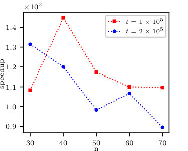 Figure 1
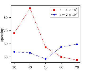 Figure 2
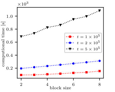 Figure 3
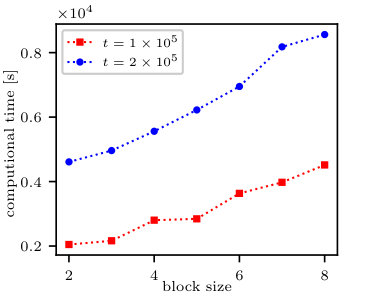 Figure 4
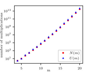 Figure 5
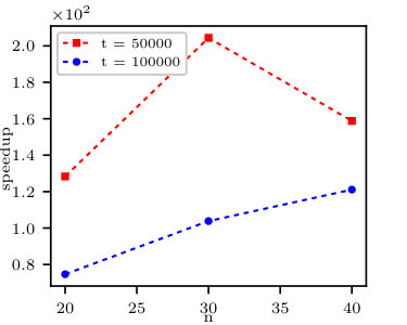 Figure 6
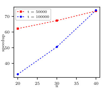 Figure 7
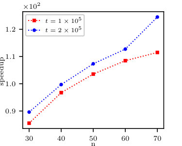 Figure 8
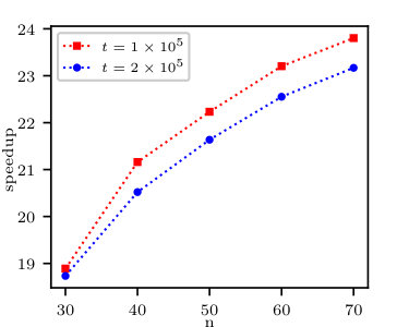 Figure 9
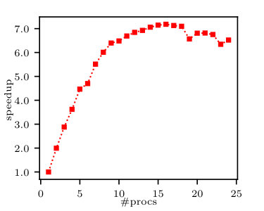 Figure 10
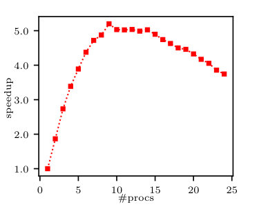 Figure 11
| Symbol | Description/explanation |
|---|---|
| element multi-index | |
| size of multi-index (number of elements) | |
| permutation of multi-index | |
| set of integers | |
| matrix of realisations of dimensional random variable | |
| vector of realisations of the th marginal random variable | |
| expectational value operator | |
| super-symmetric mode tensor of size , with elements | |
| mode tensor of sizes , with elements | |
| matrix of realisations of dimensional centered random variable | |
| the th cumulant tensor of with elements | |
| , | block of the th cumulant or moment tensor indexed by in the block structure. |
| the th central moment tensor of with elements | |
| the th moment of one dimensional |
Peer Reviews
No public reviews on file for this paper yet. If you reviewed it on a platform where reviews are public (OpenReview, ICLR, NeurIPS, ICML), you can paste yours below so the community can read it here.
Code & Models
Videos
No videos yet. Explain this paper in a talk, walkthrough, or lecture? Add one.
\newsiamthm
remarkremark \newsiamthmexampleexample
\headersComputation of higher order cumulantsKrzysztof Domino, Piotr Gawron, Łukasz Pawela
Efficient computation of higher order cumulant tensors††thanks: Submitted to the editors 07.03.2018.
\fundingThe research was partially financed by the National Science Centre, Poland—project number 2014/15/B/ST6/05204.
Krzysztof Domino Institute of Theoretical and Applied Informatics, Polish Academy of Sciences, Bałtycka 5, 44-100 Gliwice, Poland () {kdomino, gawron, lpawela}@iitis.pl
Piotr Gawron 22footnotemark: 2
Łukasz Pawela 22footnotemark: 2
keywords:
High order cumulants, non-normally distributed data, numerical algorithms
March, 7, 2018
Abstract
In this paper, we introduce a novel algorithm for calculating arbitrary order cumulants of multidimensional data. Since the th order cumulant can be presented in the form of an -dimensional tensor, the algorithm is presented using tensor operations. The algorithm provided in the paper takes advantage of super-symmetry of cumulant and moment tensors. We show that the proposed algorithm considerably reduces the computational complexity and the computational memory requirement of cumulant calculation as compared with existing algorithms. For the sizes of interest, the reduction is of the order of compared to the naïve algorithm.
{AMS}
65Y05, 15A69, 65C60
1 Introduction
1.1 Motivation
Cumulants of the order of have recently started to play an important role in the analysis of non-normally distributed multivariate data. Some potential applications of higher-order cumulants include signal filtering problems where the normality assumption is not required (see [25, 32] and references therein). Another application is finding the direction of received signals [45, 41, 10, 33] and signal auto-correlation analysis [37]. Higher-order cumulants are used in hyper-spectral image analysis [26], financial data analysis [2, 29] and neuroimage analysis [9, 5]. Outside the realm of signal analysis, higher order cumulants can be applied to quantum noise investigation purposes [24], as well as to other types of non-normally distributed data, such as weather data [15, 19, 43], various medical data [46], cosmological data [50] or data generated for machine learning purposes [22].
In the examples mentioned above only cumulants of the order of were used due to growing computational complexity and large estimation errors of high order statistics. The computational complexity and the use of computational resources increases considerably with the cumulants’ order by a factor of , where is the order of the cumulant and is the number of marginal variables.
Despite the foregoing, cumulants of order of multivariate data were successfully used in high-resolution direction-finding methods of multi-source signals (the q-MUSIC algorithm) [12, 11, 13, 34] despite higher variance of the statistic’s estimation. In such an algorithm, the number of signal sources that can be detected is proportional to the cumulant’s order [44]. Cumulants of the order of also play an important role in financial data analyses, as they enable measurement of the risk related to portfolios composed of many assets [48, 38]. This is particularly important during an economic crisis, since higher order cumulants make it possible to sample larger fluctuation of prices [42]. In [48], cumulants of the order of 2–6 of multi-asset portfolios were used as a measure of risk seeking vs. risk aversion. In [38], it was shown that, during an economic crisis, cumulants of the order of are important to analyse variations of assets and prices of portfolios. Further arguments for the utility of cumulants of the order of can be found in [28, 1] and [18] where cumulant tensors of the order of 2–6 were used to analyse financial portfolios during an economic crisis. Finally, let us consider the QCD (Quantum Chromodynamics) phase structure research area. In [23], the authors have evidenced the relevance of cumulants of the order of and of net baryon number fluctuations for the analysis of freeze-out and critical conditions in heavy ion collisions. Standard errors of those cumulant estimations were discussed in [36].
In our study, we introduce an efficient method to calculate higher-order cumulants. This method takes advantage of the recursive relation between cumulants and moments as well as their super-symmetric structure. These features enable us to reduce the computational complexity of the naïve algorithm and make the problem tractable. In order to reduce complexity, we use the idea introduced in [49] to decrease the storage and computational requirements by a factor of .
This allows us to handle large data sets and overcome a major problem in numerical handling of high order moments and cumulants. Consider that the estimation error of the one-dimensional th central moment is limited from above by where is the th central moment and is number of data samples. This is discussed further in Appendix A. Consequently, the accurate estimation of statistics of the order of requires correspondingly large data sets. In practice, our approach allows us to handle cumulants up to the tenth order.
1.2 Normally and non-normally distributed data
Let us consider the -dimensional normally distributed random variable where is a positive-definite covariance matrix and is a mean value vector. In this case, the characteristic function and cumulant generating function [30, 35] are
[TABLE]
It is easy to see that is quadratic in , and therefore its third and higher derivatives with respect to are zero. As we will in the next section, this implies that cumulants of order greater than two are equal to zero.
If data is characterised by a frequency distribution other than the multivariate normal distribution, the characteristic function may be expanded in more terms than quadratic, and cumulants of the order higher than two may have non-zero elements. This is why they are helpful in distinguishing between normally and non-normally distributed data or between data from different non-normal distributions.
1.3 Basic definitions
Let us start with a random process generating discrete dimensional values. A sequence of samples of an dimensional random variable is represented in the form of matrix such that
[TABLE]
This matrix can be represented as a sequence of vectors of realisations of marginal variables
[TABLE]
where
[TABLE]
In order to study moments and cumulants of , we need the notion of super-symmetric tensors. Let us first denote the set as , a permutation of tuple as .
Definition 1.1**.**
Let be a tensor with elements indexed by multi-index . Tensor is super-symmetric iff it is invariant under any permutation of the multi-index, i.e.
[TABLE]
Henceforth we will write for super-symmetric tensor . A list of all notations used in this paper is provided in Table 1.
Definition 1.2**.**
Let be as in Eq. (2). We define the th moment as tensor . Its elements are indexed by multi-index and equal
[TABLE]
*where is the expectational value operator and a vector of realisations of the th marginal variable. *
Definition 1.3**.**
Let be as in Eq. (2). We define centered variable as
[TABLE]
The first two cumulants respectively correspond to the mean vector and the symmetric covariance matrix of . Given the following estimator:
[TABLE]
we first introduce the definition of cumulants of arbitrary order and later explicitly state definitions for cumulants of order one to four [30, 35]
Definition 1.4**.**
Let be a multi-index with elements , and the cumulant generation function of a given distribution. The th cumulant element is defined by [30, 35]
[TABLE]
*we drop an imaginary unit in definition for a presentation clarity. *
Definition 1.5**.**
We define the first cumulant as
[TABLE]
Definition 1.6**.**
We define the second cumulant as
[TABLE]
Definition 1.7**.**
We define the third cumulant as a three-mode tensor with elements
[TABLE]
Cumulants of order greater than three can be computed from moments [40, 39], however the relation is complex and requires a special notation which is introduced in Subsection 3.1. To show how complicated the formulas might become we state here the partial formula for the fourth cumulant.
Definition 1.8**.**
We define the fourth cumulant as a four-mode tensor with elements
[TABLE]
Switching to the centered variable , using a fact that , and for , cumulants of order greater than one are mean shift invariant [39], we can write Eq. (13) in a following manner:
[TABLE]
Remark 1.9**.**
*Each cumulant tensor as well as each moment tensor is super-symmetric [4]. *
As the formula for a cumulant of an arbitrary order is very complex, our core result is the numerical handling of a cumulant and is discussed in depth in Section 3. To compute cumulant tensor of order we use central moment tensors of order and and take advantage of cumulant and moment tensors super-symmetry. Importantly we do not need to determine th moment tensor.
2 Moment tensor calculation
To provide a simpler example, we start with algorithms for calculation of the moment tensor. Next, in Section 3, those algorithms will be utilised to recursively calculate the cumulants.
2.1 Storage of super-symmetric tensors in block
structures
In this section, we are going to follow the idea introduced by Schatz et al. [49] concerning the use of blocks to store symmetric matrices and super-symmetric tensors in an efficient way. To make the demonstration more accessible, we will first focus on the matrix case. Let us suppose we have symmetric matrix . We can store the matrix in blocks and store only upper triangular blocks,
[TABLE]
where NULL represents an empty block, and . Entries below the diagonal do not need to be stored and calculated as they are redundant. Each block is of size . Blocks are of size , and block is of size , where:
[TABLE]
This representation significantly reduces the overall storage footprint while still providing opportunities to achieve high computational performance.
This representation can easily be extended for purposes of super-symmetric tensors. Let us assume that is a super-symmetric tensor. All data can be stored in blocks . If indices are not sorted in an increasing order, such blocks are redundant and consequently replaced by NULL. Similarly to the matrix case we have
[TABLE]
In the subsequent sections we present algorithms for moment and cumulant tensor calculation and storage. For simplicity, we assume that and . The generalization is straightforward and, at this point, would only obscure the main idea.
Henceforth each block is a hypercube of size and there are such unique blocks [49]. Such storage scheme, proposed in [49], requires the storage of elements.
2.2 The algorithm
In this and following sections, we present the moment and cumulant calculation algorithms that use the block structure. To compute the th moment tensor we use Def. 1.2. Algorithm 1 computes a single block of the tensor, while Algorithm 2 computes the whole tensor in the block structure form.
Based on [49] and the discussion in the previous subsection, we can conclude that reduction of redundant blocks reduces the storage and computational requirements of the th moment tensor by a factor of for compared to the naïve algorithm. The detailed analysis of the computational requirements will be presented in Section 5.
2.3 Parallel computation of moment tensor
For large , it is desirable to speedup the moment tensor calculation further. This can be achieved via a simple parallel scheme. Let us suppose for the sake of simplicity, that we have processes available, and . Starting with data we can split them into non overlapping subsets . In the first step, for each subset, we compute in parallel moment tensor using Algorithm 2. In the second step, we perform the following reduction
[TABLE]
The elements of the tensor under the sum on the RHS are
[TABLE]
The element of the moment tensor of is
[TABLE]
These steps are summarised in Algorithm 3.
3 Calculation of cumulant tensors
At this point, we can define our main result, i.e. an algorithm for calculating cumulants of arbitrary order of multi-dimensional data.
3.1 Index partitions and permutations
In this section, we present a recursive formula that can be used to calculate the th cumulant of . We begin with some definitions, mainly concerning combinatorics, before discussing the general formula.
Definition 3.1**.**
Let , and . Partition of tuple is the division of into non-crossing sub-tuples: ,
[TABLE]
In what follows, we will denote the permutations of a tuple of tuples , as .
Definition 3.2**.**
* — the representative of the equivalence class of partitions. Let and be partitions of . Let us introduce the following equivalence relation:*
[TABLE]
*This relation defines the equivalence class. Henceforth we will take only one representative of each equivalence class and denote it as . The representative will be such that all are sorted in an increasing order. We will denote a set of all such equivalence classes as . *
Remark 3.3**.**
The number of partitions of set of size into parts is given by the Stirling Number of the second kind, [27]
[TABLE]
Definition 3.4**.**
Consider tensors , indexed by and respectively. Their outer product is defined as
[TABLE]
*where denotes multi-index . *
As an example consider the outer product of symmetric matrix by itself: , that is only partially symmetric, , but in general . To obtain a super-symmetric outcome of the outer product of super-symmetric tensors, we need to apply the following symmetrisation procedure.
Definition 3.5**.**
The sum of outer products of super-symmetric tensors. Let be a tensor indexed by . Let be a sub-tuple of its modes according to Def. 3.2, and let . For the given , we define the sum of outer products of where and , using the elementwise notation, as
[TABLE]
We will use the following abbreviation using tensor notation
[TABLE]
Consider as in Eq. (26) where are super-symmetric and iff and is a multi-index of . The sum over all representatives of equivalence classes fully symmetrises the outer product, and therefore is super-symmetric. In other words, due to the super-symmetry, any permutation of multi–index of that leads only to a permutation of indices inside some refers to the same value of . Any permutation of that leads only to the switch between and inside an outer product in Eq. (26) also refers to the same value of . Any other permutation of that cannot be represented as above switches between equivalence classes as well, and so it switches between elements of sum Eq. (26) and refers to the same value of .
Example 3.6**.**
Consider , and such that
[TABLE]
then
[TABLE]
*such is super-symmetric, since there is no permutation of that changes its elements, i.e. . *
3.2 Cumulant calculation formula
The following recursive relation can be used to relate moments and cumulants of :
[TABLE]
This can be written in an elementwise manner as in [4]
[TABLE]
For the sake of completeness, we present an alternative proof of Eq. (30) in Appendix B.
In order to compute , let us consider the case where separately. By definition, , so:
[TABLE]
The th cumulant tensor can be calculated given the th moment tensor and cumulant tensors of the order of
[TABLE]
To simplify Eq. (32), let us observe that cumulants of the order of two or higher for a non-centered variable and a centered variable are equal. The first order cumulant for a centered variable is zero. Hereafter, we introduce partitions into sub-tuples of size larger than one.
Definition 3.7**.**
Let , and . The at least two element partition of tuple is the division of into sub-tuples: , such that
[TABLE]
The definition of the representative of equivalence class and the set of such representatives are analogous to Def. 3.2. Consequently, we can derive the final formula
[TABLE]
Let us determine the limit. If is even, it can be divided into at most parts of size two; if is odd, it can be divided into at most parts: parts of size two and one part of size three. Hence we can conclude that .
As a simple example, consider the cumulants of the order of three and four. Since , then and , i.e. the second cumulant matrix and the third cumulant tensor are simply the second and the third central moments. Formulas for cumulant tensors of the order greater than three are more complicated. For example, consider the th cumulant tensor
[TABLE]
Using the elementwise notation, where , we have
[TABLE]
3.3 Algorithms to compute cumulant tensors
Let us suppose that is the th element of the th block of the super–symmetric tensor of the order of . Similarly, is the th element of the th block of the th cumulant tensor according to Def. 3.5—we skip now in for brevity. With reference to Def. 3.5 and Def. 3.2, is always sorted and from the properties of the block structure is also sorted, hence is sorted as well. To determine we use modified Knuth’s algorithm [31]. Now we have all the components to introduce Algorithm 4 which computes a super-symmetric sum of outer products of lower order cumulants. Algorithm 4 computes the inner sum of Eq. (34) and takes advantages of the super-symmetry of tensors by using the block structure.
Finally, Algorithm 5 computes the th cumulant tensor. It uses Eq. (34) to calculate the cumulants and importantly takes advantage of the super-symmetry of tensors, because it refers to Algorithm 2 (moment tensor calculation) and Algorithm 4 that both use the block structure.
4 Implementation
All algorithms presented in this paper are implemented in the Julia programming language [8, 7]. Julia is a high level language in which multi-dimensional tables are first class types [6]. For purposes of the algorithms, two modules were created. In the first one, SymmetricTensors.jl, [21] the block structure of super-symmetric tensors was implemented. In the second module, Cumulants.jl, [20] we used the block structure to compute and store moment and cumulant tensors. The implementation of cumulants calculation uses multiprocessing primitives built into the Julia programming language: remote references and remote calls. A remote reference is an object that allows any process to reference an object stored in a specific process. A remote call allows a process to request a function call on certain arguments on another process.
5 Performance analysis
This section is dedicated to the performance analysis of the core elements of our algorithms. These are Eq. (6) which calculates the moment tensor and Eq. (34) which calculates the cumulant tensor. First, we discuss theoretical analysis and then focus on the performance of our implementation. In the final subsection, we show how our implementation compares to the current state of the art.
5.1 Theoretical analysis
We start by discussing the performance of the moment tensor. With reference to Section 2, let us recall that storage of the moment tensor requires storage of the floating-point numbers. We can approximate for [49]. Since we usually calculate cumulants of the order of and we deal with high dimensional data, we need approximately of the computer storage space, compared with the naïve storage scheme.
As for the cumulants, one should primarily note that the number of elements of the inner sum in Eq. (34) in the second line equals the number of set partitions of into exactly parts, such that no part is of size one, and can be represented as:
[TABLE]
We call it a modification of the Stirling number of the second kind , and compute it as follows
[TABLE]
where we count the number of ways to divide elements into subsets of length such that , and so . Factor in the denominator counts the number of subset permutations. Some examples of are , , and .
The following sum
[TABLE]
is the number of all partitions of a set of size into subsets, such that there is no subset of size one, and therefore
[TABLE]
Here is a Bell number [14], the number of all partitions of a set of size including subsets of size one and is the number of partitions of a set of size into subsets such that at least one subset is of size one. Relation Eq. (40) is derived from the fact that there is a bijective relation between partitions of element set into subsets such that at least one subset is of size one and partitions of element set into subsets such that there is no subset of size one.
To compute each element of the inner sum in Eq. (34), we need multiplications, and consequently to compute each element of the outer sum in Eq. (34), we need multiplications. Finally, the number of multiplications required to compute the second term of the RHS of Eq. (34) is
[TABLE]
for each tensor element. Let us note that , , . The plot of and the upper bound are shown in Fig. 1. From Fig. 1 the proposed upper bound produces a very good approximation of the number of multiplications.
From Eq. (6), Eq. (34) and Eq. (41) we can conclude that to compute the th cumulant’s element we need multiplications for the central moment and multiplications for the sums in Eq. (34). However, in order to calculate the cumulant in an accurate manner, we need large data sets, i.e. for we use and for the data size must be even larger. Bearing in mind that computation of cumulants of the order of is inapplicable, the foregoing gives . Henceforth dominant computational power is required to calculate the moment tensor, so there appears the need for approximately multiplications to compute each th cumulant’s element. To compute the whole th cumulant tensor we need approximately multiplications, while the factor is a result of taking advantage of super-symmetry. The added cost due to blocking is negligible, see [49].
It is now possible to compare the complexity of our algorithm with that of the naïve algorithm for chosen cumulants. For the th cumulant, the naïve algorithm would use Eq. (14) directly and would not take advantage of the super-symmetry of tensors. Therefore, it requires multiplications to compute a single cumulant tensor element and multiplications to compute the whole cumulant tensor. Our algorithm, in this case, decreases the computational complexity by the factor of .
Analogically, the naïve formula for the th cumulant
[TABLE]
requires approximately multiplications to compute the whole cumulant tensor. Our algorithm, in this case, decreases the computational complexity by the factor of . For higher , the difference is even greater due to the factor caused by the application of the block structure and the fact that the number of terms in naïve formulas grows with much faster than from Eq. (40).
5.2 Implementation performance
In this section, we analyse the performance analysis of our implementation. All computations were performed in the Prometheus computing cluster. This cluster provides shared user access with multiple user tasks running on each node. Each node is an HP XL730f Gen9 computing system with dual Intel Xeon E5-2680v3 processors providing 12 physical cores and 24 computing cores with hyper-threading. The node has 128 GB of memory.
5.2.1 The optimal size of blocks
The number of coefficients required to store a super-symmetric tensor of order and dimensions is equal to . The storage of tensor disregarding the super-symmetry requires coefficients. The block structure introduced in [49] uses more than minimal amount of memory but allows for easier further processing of super-symmetric tensors.
If we store the super-symmetric tensor in the block structure, the block size parameter appears. In our implementation in order to store a super-symmetric tensor in the block structure we need, assuming , an array of pointers to blocks and an array of the same size of flags that contain the information if a pointer points to a valid block. Recall that diagonal blocks contain redundant information. Therefore on the one hand, the smaller the value of , the less redundant elements on diagonals of the block structure. On the other hand, the larger the value of , the smaller the number of blocks, the smaller the blocks’ operation overhead, and the fewer the number of pointers pointing to empty blocks. For detailed discussion of memory usage see [49]. The analysis of the influence of the parameter on the computational time of cumulants for some parameters are presented in Fig. 2. We obtain the shortest computation time for in almost all test cases, and this value will be set as default and used in all efficiency tests. Note that for we loose all the memory savings.
5.2.2 Comparison with naïve algorithms
The computational speedup of cumulant calculation for the illustrative data is presented in Fig. 3. The computational speedup is even higher than the theoretical value of , which is probably due to large operational memory requirements and some computational overhead while splitting data into terms of Eq. (36) used by the naïve approach.
As for the moment calculation, let us recall from Section 2.1 that we expect a speedup on the level of . As can be shown in Fig 4, this is the case for a high number of marginal variables , as we approach speedup equal to for the fourth moment. This is a case, since there is some redundancy in computation of diagonal blocks which decreases as rises, given .
5.2.3 Multiprocessing performance
In this section we analyse the multiprocessing performance of moment tensor calculations, since according to Subsection 5.1, the moment tensor calculation takes the majority of cumulants calculation time. Fig. 5 shows the speedup of multiprocess moment calculation compared to single process calculation. As can be shown in the figure, at first, we obtain linear scaling of the speedup with the number of processes. Next, we reach the saturation point. This is expected, as there are some parts of this calculation that cannot be done in parallel. Adding more processes leads to a drop in the speedup. This is due to the fact that adding more processes results in more overall overhead, yet we do not benefit from splitting the data further.
5.3 Comparison with the state of the art
The state of the art in terms of the cumulant calculation simplification is referred to as umbral calculus [47], which is a formal system consisting of certain operations on objects called umbrae, mimicking addition and multiplication of independent real-valued random variables. Using umbrae notation one can determine symbolic formulas to calculate elements of cumulant tensors. See [17] where cumulants, also called -statistics, were derived using purely combinatorial operations. However, symbolic computations are less universal and sometimes problematic, while translating them into algorithms and code is not entirely straightforward.
We present a more general approach by implementing an algorithm that takes multivariate data in the form of a matrix and computes its cumulant tensors. The current state of the art is a package written in the R programming language [16]. This algorithm uses the recursion relation to compute the th cumulant from moments of the order of [40, 39, 3], see Eq. (43).
[TABLE]
where is the number of parts in the given partition . The algorithm computes each element of cumulant tensors, without taking advantage of their super-symmetry. For comparison, our formula, i.e. Eq. (34) is simpler, as it lacks factor and the inner sum has less elements, since we have introduced instead of . Further application of Eq. (34) enables us to compute the th cumulant tensor without determining the th moment tensor. This fact can be advantageous in high-resolution direction-finding methods for multi-source signals (the q-MUSIC algorithm) [12] where one needs a cumulant of the order of but not a cumulant and a moment of the order of . Furthermore, the major benefit of our algorithm is the utilisation of the super-symmetry of cumulant tensors. By introducing blocks, the computational complexity can be reduced by a factor of in the same manner as the storage requirement is reduced.
In [16] two algorithms were implemented: one—four_cumulants_direct—that uses a direct formula for cumulants of orders — which we call the specialized algorithm, and other one—cumulants_upto_p—that can compute cumulants of arbitrary order using Eq. (43), which we call the general algorithm. Both of these algorithms were implemented in the R programming language. The specialized algorithm outperforms the general one in terms of speed. For comparison’s sake, we re-implemented the general algorithm from [16] in Julia maintaining high similarity between both implementations.
To perform the efficiency comparison, we compare the computational time of our algorithm with the aforementioned algorithms. The obtained results are summarised in Fig. 6 which contains:
- •
The comparison of our algorithm and the general algorithm [16] re-implemented in Julia—Fig. 6(a).
- •
The comparison between our algorithm and the general algorithm implemented in [16]—Fig. 6(b). Our algorithm is faster by two orders of magnitude owing to the fact that there exists acceleration factor. It results from the utilisation of super-symmetry through application the block structure. It turns out that our implementation achieves in practice even higher acceleration.
- •
The comparison of our algorithm vs. the specialised algorithm implemented in [16]—Fig. 6(c).
6 Conclusions
This paper provides a discussion on both the method and the algorithm for calculation of arbitrary order moment and cumulant tensors given multidimensional data. To this end, we introduce the recurrence relation between the th cumulant tensor and the th central moment tensor as well as cumulant tensors of the order of . For purposes of efficient computation and storage of super-symmetric tensors, we use blocks to store and calculate only the pyramidal part of cumulant and moment tensors. Our algorithm is significantly faster than the existing algorithms. The theoretical speedup is given by the factor of , which makes the algorithm applicable in the analysis of large data sets. Another important aspect is that large data sets are required to approximate accurately high order statistics on account of their large approximation error. If the estimation error challenge is successfully tackled, high order multidimensional statistics such as high order moments or cumulants will be an important tool to analyse non-normally distributed data, where the mean vector and the covariance matrix contain little information about the data. There are many applications of such statistics, particularly involving signal analysis, financial data analysis, hyper-spectral data analysis or particle physics.
Appendix A The estimation error of high order statistics
Let be an estimator of the th moment of one-dimensional centered random variable , and let us have available realisations of . As we consider large , the bias of such an estimator can be neglected as being much smaller than a standard error. Hence, we can use the following estimator
[TABLE]
where we just sum independent random variables raised to the power of . The variance of can be represented as:
[TABLE]
Since are independent and equal in distribution to ,
[TABLE]
hence
[TABLE]
and obviously this limit is relevant if exists. In the multivariate case are only independent in groups. The number of groups can be estimated using the number of marginal variables , but still . Consequently, a similar limitation can be expected, but replacing with a product of moments of lower orders.
Appendix B The recurrence formula for cumulant calculations
We recall the cumulant generating function
[TABLE]
which is related to the moment generation (characteristic) function , For simplicity, we use the following notation: , , and drop in notation . The elements of the moment and cumulant tensor at multi-index are
[TABLE]
We have the following theorem
Proposition B.1**.**
For each the following holds:
[TABLE]
Proof B.2**.**
For the results follow from direct inspection. Next, for we get:
[TABLE]
Now assume that Eq. (50) holds for . Differentiating its LHS, we have
[TABLE]
further using Eq. (50) we obtain , therefore
[TABLE]
where . After differentiating Eq. (49), we have
[TABLE]
and analogously
[TABLE]
Differentiating the RHS of Eq. (50),
[TABLE]
comparing Eq. (56) with Eq. (53), we have
[TABLE]
Finally, we obtain
[TABLE]
If we observe that \tilde{\phi}(\tau)\big{|}_{\tau=0}=1 and m_{\mathbf{i}}=\partial_{\mathbf{i}}\tilde{\phi}(\tau)\big{|}_{\tau=0} and c_{\mathbf{i}}(\tau)\big{|}_{\tau=0}=c_{\mathbf{i}}, then Eq. (50) at will give Eq. (30).
Acknowledgements
The authors would like to thank Adam Glos for revising the manuscript and Zbigniew Puchała for the discussion about error estimation and set partitions. This research was supported in part by PL-Grid Infrastructure
The reference list from the paper itself. Each links out to its DOI / PubMed record.
- 1[1] G. S. Amin and H. M. Kat , Hedge Fund Performance 1990-2000: Do the “Money Machines" Really Add Value? , Journal of financial and quantitative analysis, 38 (2003), pp. 251–274.
- 2[2] J. C. Arismendi and H. Kimura , Monte Carlo Approximate Tensor Moment Simulations , Available at SSRN 2491639, (2014).
- 3[3] N. Balakrishnan, N. L. Johnson, and S. Kotz , A note on relationships between moments, central moments and cumulants from multivariate distributions , Statistics & probability letters, 39 (1998), pp. 49–54.
- 4[4] O. E. Barndorff-Nielsen and D. R. Cox , Asymptotic techniques for use in statistics , Chapman & Hall, 1989.
- 5[5] H. Becker, L. Albera, P. Comon, M. Haardt, G. Birot, F. Wendling, M. Gavaret, C.-G. Bénar, and I. Merlet , EEG extended source localization: tensor-based vs. conventional methods , Neuro Image, 96 (2014), pp. 143–157.
- 6[6] J. Bezanson, J. Chen, S. Karpinski, V. Shah, and A. Edelman , Array operators using multiple dispatch: A design methodology for array implementations in dynamic languages , in Proceedings of ACM SIGPLAN International Workshop on Libraries, Languages, and Compilers for Array Programming, ACM, 2014, p. 56.
- 7[7] J. Bezanson, A. Edelman, S. Karpinski, and V. B. Shah , Julia: A fresh approach to numerical computing , SIAM Review, 59 (2017), pp. 65–98.
- 8[8] J. Bezanson, S. Karpinski, V. B. Shah, and A. Edelman , Julia: A fast dynamic language for technical computing , ar Xiv:1209.5145, (2012).
