TL;DR
This paper introduces a scalable matrix-factorization algorithm that efficiently handles massive matrices by streaming and subsampling, with proven convergence and demonstrated success on large real-world datasets.
Contribution
The proposed method combines streaming and subsampling techniques for scalable matrix factorization with convergence guarantees, suitable for large-scale data and various factor types.
Findings
Achieves significant speed-ups over state-of-the-art algorithms.
Successfully applied to 2 TB MRI data and 103 GB hyperspectral images.
Provides convergence guarantees to a stationary point.
Abstract
We present a matrix-factorization algorithm that scales to input matrices with both huge number of rows and columns. Learned factors may be sparse or dense and/or non-negative, which makes our algorithm suitable for dictionary learning, sparse component analysis, and non-negative matrix factorization. Our algorithm streams matrix columns while subsampling them to iteratively learn the matrix factors. At each iteration, the row dimension of a new sample is reduced by subsampling, resulting in lower time complexity compared to a simple streaming algorithm. Our method comes with convergence guarantees to reach a stationary point of the matrix-factorization problem. We demonstrate its efficiency on massive functional Magnetic Resonance Imaging data (2 TB), and on patches extracted from hyperspectral images (103 GB). For both problems, which involve different penalties on rows and columns,…
Click any figure to enlarge with its caption.
 Figure 1
 Figure 2
 Figure 3
 Figure 4
 Figure 5
 Figure 6
 Figure 7
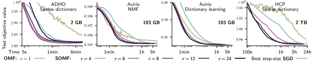 Figure 8
 Figure 9
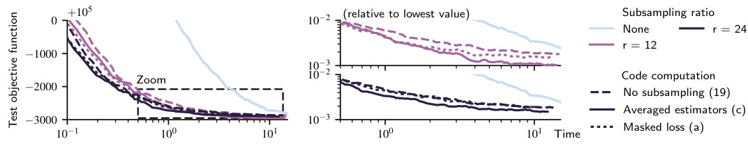 Figure 10
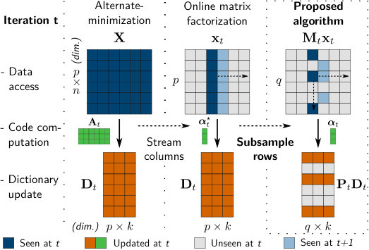 Figure 11
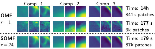 Figure 12
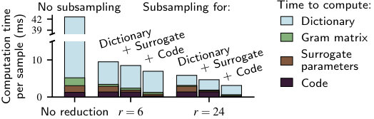 Figure 13
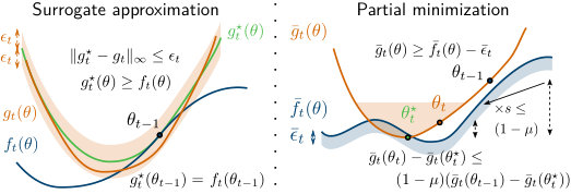 Figure 14
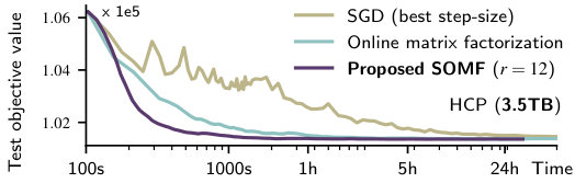 Figure 15
| Field | Functional MRI | Hyperspectral imaging | |
|---|---|---|---|
| Dataset | ADHD | HCP | Patches from AVIRIS |
| Factors | sparse, dense | dense, sparse | |
| # samples | |||
| # features | |||
| size | 2 GB | 2 TB | 103 GB |
| Use case ex. | Extracting predictive feature | Recognition / denoising | |
| Dataset | ADHD | AVIRIS (NMF) | AVIRIS (DL) | HCP | ||||
| Algorithm | omf | somf | omf | somf | omf | somf | omf | somf |
| Conv. time | ||||||||
| Speed-up | 11.8 | 3.36 | 6.80 | 13.31 | ||||
Peer Reviews
No public reviews on file for this paper yet. If you reviewed it on a platform where reviews are public (OpenReview, ICLR, NeurIPS, ICML), you can paste yours below so the community can read it here.
Code & Models
Videos
No videos yet. Explain this paper in a talk, walkthrough, or lecture? Add one.
Stochastic Subsampling for
Factorizing Huge Matrices
Arthur Mensch, Julien Mairal,
Bertrand Thirion, and Gaël Varoquaux A. Mensch, B. Thirion, G. Varoquaux are with Parietal team, Inria, CEA, Paris-Saclay University, Neurospin, at Gif-sur-Yvette, France. J. Mairal is with Université Grenoble Alpes, Inria, CNRS, Grenoble INP, LJK at Grenoble, France. The research leading to these results was supported by the ANR (MACARON project, ANR-14-CE23-0003-01 — NiConnect project, ANR-11-BINF-0004NiConnect). It has received funding from the European Union’s Horizon 2020 Framework Programme for Research and Innovation under Grant Agreement No 720270 (Human Brain Project SGA1). Corresponding author: Arthur Mensch ([email protected])
Abstract
We present a matrix-factorization algorithm that scales to input matrices with both huge number of rows and columns. Learned factors may be sparse or dense and/or non-negative, which makes our algorithm suitable for dictionary learning, sparse component analysis, and non-negative matrix factorization. Our algorithm streams matrix columns while subsampling them to iteratively learn the matrix factors. At each iteration, the row dimension of a new sample is reduced by subsampling, resulting in lower time complexity compared to a simple streaming algorithm. Our method comes with convergence guarantees to reach a stationary point of the matrix-factorization problem. We demonstrate its efficiency on massive functional Magnetic Resonance Imaging data (2 TB), and on patches extracted from hyperspectral images (103 GB). For both problems, which involve different penalties on rows and columns, we obtain significant speed-ups compared to state-of-the-art algorithms.
Index Terms:
Matrix factorization, dictionary learning, NMF, stochastic optimization, majorization-minimization, randomized methods, functional MRI, hyperspectral imaging
I Introduction
Matrix factorization is a flexible approach to uncover latent factors in low-rank or sparse models. With sparse factors, it is used in dictionary learning, and has proven very effective for denoising and visual feature encoding in signal and computer vision [see e.g., 1]. When the data admit a low-rank structure, matrix factorization has proven very powerful for various tasks such as matrix completion [2, 3], word embedding [4, 5], or network models [6]. It is flexible enough to accommodate a large set of constraints and regularizations, and has gained significant attention in scientific domains where interpretability is a key aspect, such as genetics [7] and neuroscience [8]. In this paper, our goal is to adapt matrix-factorization techniques to huge-dimensional datasets, i.e., with large number of columns and large number of rows . Specifically, our work is motivated by the rapid increase in sensor resolution, as in hyperspectral imaging or fMRI, and the challenge that the resulting high-dimensional signals pose to current algorithms.
As a widely-used model, the literature on matrix factorization is very rich and two main classes of formulations have emerged. The first one addresses a convex-optimization problem with a penalty promoting low-rank structures, such as the trace or max norms [2]. This formulation has strong theoretical guarantees [3], but lacks scalability for huge datasets or sparse factors. For these reasons, our paper is focused on a second type of approach, which relies on nonconvex optimization. Stochastic (or online) optimization methods have been developed in this setting. Unlike classical alternate minimization procedures, they learn matrix decompositions by observing a single matrix column (or row) at each iteration. In other words, they stream data along one matrix dimension. Their cost per iteration is significantly reduced, leading to faster convergence in various practical contexts. More precisely, two approaches have been particularly successful: stochastic gradient descent [9] and stochastic majorization-minimization methods [10, 11]. The former has been widely used for matrix completion [see 12, 13, 14, and references therein], while the latter has been used for dictionary learning with sparse and/or structured regularization [15]. Despite those efforts, stochastic algorithms for dictionary learning are currently unable to deal efficiently with matrices that are large in both dimensions.
We propose a new matrix-factorization algorithm that can handle such matrices. It builds upon the stochastic majorization-minimization framework of [10], which we generalize for our problem. In this framework, the objective function is minimized by iteratively improving an upper-bound surrogate of the function (majorization step) and minimizing it to obtain new estimates (minimization step). The core idea of our algorithm is to approximate these steps to perform them faster. We carefully introduce and control approximations, so to extend convergence results of [10] when neither the majorization nor the minimization step is performed exactly.
For this purpose, we borrow ideas from randomized methods in machine learning and signal processing. Indeed, quite orthogonally to stochastic optimization, efficient approaches to tackle the growth of dataset dimension have exploited random projections [16, 17] or sampling, reducing data dimension while preserving signal content. Large-scale datasets often have an intrinsic dimension which is significantly smaller than their ambient dimension. Good examples are biological datasets [18] and physical acquisitions with an underlying sparse structure enabling compressed sensing [19]. In this context, models can be learned using only random data summaries, also called sketches. For instance, randomized methods [see 20, for a review] are efficient to compute PCA [21], a classic matrix-factorization approach, and to solve constrained or penalized least-square problems [22, 23]. On a theoretical level, recent works on sketching [24, 25] have provided bounds on the risk of using random summaries in learning.
Using random projections as a pre-processing step is not appealing in our applicative context since factors learned on reduced data are not interpretable. On the other hand, it is possible to exploit random sampling to approximate the steps of online matrix factorization. Factors are learned in the original space whereas the dimension of each iteration is reduced together with the computational cost per iteration.
Contribution
The contribution of this paper is both practical and theoretical. We introduce a new matrix factorization algorithm, called subsampled online matrix factorization (somf), which is faster than state-of-the-art algorithms by an order of magnitude on large real-world datasets (hyperspectral images, large fMRI data). It leverages random sampling with stochastic optimization to learn sparse and dense factors more efficiently. To prove the convergence of somf, we extend the stochastic majorization-minimization framework [10] and make it robust to some time-saving approximations. We then show convergence guarantees for somf under reasonable assumptions. Finally, we propose an extensive empirical validation of the subsampling approach.
In a first version of this work [26] presented at the International Conference in Machine Learning (icml), we proposed an algorithm similar to somf, without any theoretical guarantees. The algorithm that we present here has such guarantees, which we express in a more general framework, stochastic majorization-minimization. It is validated for new sparsity settings and a new domain of application. An open-source efficient Python package is provided.
Notations
Matrices are written using bold capital letters and vectors using bold small letters (e.g., , ). We use superscript to specify the column (sample or component) number, and write . We use subscripts to specify the iteration number, as in . The floating bar, as in , is used to stress that a given value is an average over iterations, or an expectation. The superscript ⋆ is used to denote an exact value, when it has to be compared to an inexact value, e.g., to compare (exact) to (approximation).
II Prior art: matrix factorization with stochastic
majorization-minimization
Below, we introduce the matrix-factorization problem and recall a specific stochastic algorithm to solve it observing one column (or a mini-batch) at every iteration. We cast this algorithm in the stochastic majorization-minimization framework [10], which we will use in the convergence analysis.
II-A Problem statement
In our setting, the goal of matrix factorization is to decompose a matrix — typically signals of dimension — as a product of two smaller matrices:
[TABLE]
with potential sparsity or structure requirements on and . In signal processing, sparsity is often enforced on the code , in a problem called dictionary learning [27]. In such a case, the matrix is called the “dictionary” and the sparse code. We use this terminology throughout the paper.
Learning the factorization is typically performed by minimizing a quadratic data-fitting term, with constraints and/or penalties over the code and the dictionary:
[TABLE]
where , is a column-wise separable convex set of and is a penalty over the code. Both constraint set and penalty may enforce structure or sparsity, though has traditionally been used as a technical requirement to ensure that the penalty on does not vanish with growing arbitrarily large. Two choices of and are of particular interest. The problem of dictionary learning sets as the ball for each atom and to be the norm. Due to the sparsifying effect of penalty [28], the dataset admits a sparse representation in the dictionary. On the opposite, finding a sparse set in which to represent a given dataset, with a goal akin to sparse PCA [29], requires to set as the ball for each atom and to be the norm. Our work considers the elastic-net constraints and penalties [30], which encompass both special cases. Fixing and in , we denote by and the elastic-net penalty in and :
[TABLE]
Following [15], we can also enforce the positivity of and/or by replacing by in , and adding positivity constraints on in (1), as in non-negative sparse coding [31]. We rewrite (1) as an empirical risk minimization problem depending on the dictionary only. The matrix solution of (1) is indeed obtained by minimizing the empirical risk
[TABLE]
and the matrix is obtained by solving the linear regression
[TABLE]
The problem (1) is non-convex in the parameters , and hence (3) is not convex. However, the problem (1) is convex in both and when fixing one variable and optimizing with respect to the other. As such, it is naturally solved by alternate minimization over and , which asymptotically provides a stationary point of (3). Yet, has typically to be observed hundred of times before obtaining a good dictionary. Alternate minimization is therefore not adapted to datasets with many samples.
II-B Online matrix factorization
When has a large number of columns but a limited number of rows, the stochastic optimization method of [15] outputs a good dictionary much more rapidly than alternate-minimization. In this setting [see 32], learning the dictionary is naturally formalized as an expected risk minimization
[TABLE]
where is drawn from the data distribution and forms an i.i.d. stream . In the finite-sample setting, (5) reduces to (3) when is drawn uniformly at random from . We then write the sample number selected at time .
The online matrix factorization algorithm proposed in [15] is summarized in Alg. 1. It draws a sample at each iteration, and uses it to improve the current iterate . For this, it first computes the code associated to on the current dictionary:
[TABLE]
Then, it updates to make it optimal in reconstructing past samples from previously computed codes :
[TABLE]
Importantly, minimizing is equivalent to minimizing the quadratic function
[TABLE]
where and are small matrices that summarize previously seen samples and codes:
[TABLE]
As the constraints have a separable structure per atom, [15] uses projected block coordinate descent to minimize . The function gradient writes , and it is therefore enough to maintain and in memory to solve (7). and are updated online, using the rules (8) (Alg. 1).
The function is an upper-bound surrogate of the true current empirical risk, whose definition involves the regression minima computed on current dictionary :
[TABLE]
Using empirical processes theory [33], it is possible to show that minimizing at each iteration asymptotically yields a stationary point of the expected risk (5). Unfortunately, minimizing (11) is expensive as it involves the computation of optimal current codes for every previously seen sample at each iteration, which boils down to naive alternate-minimization.
In contrast, is much cheaper to minimize than , using block coordinate descent. It is possible to show that converges towards a locally tight upper-bound of the objective and that minimizing at each iteration also asymptotically yields a stationary point of the expected risk (5). This establishes the correctness of the online matrix factorization algorithm (omf). In practice, the omf algorithm performs a single pass of block coordinate descent: the minimization step is inexact. This heuristic will be justified by our theoretical contribution in Section IV.
Extensions
For efficiency, it is essential to use mini-batches of size instead of single samples in the iterations [15]. The surrogate parameters , are then updated by the mean value of over the batch. The optimal size of the mini-batches is usually close to . (8) uses the sequence of weights to update parameters and . [15] replaces these weights with a sequence , which can decay more slowly to give more importance to recent samples in . These weights will prove important in our analysis.
II-C Stochastic majorization-minimization
Online matrix factorization belongs to a wider category of algorithms introduced in [10] that minimize locally tight upper-bounding surrogates instead of a more complex objective, in order to solve an expected risk minimization problem. Generalizing online matrix factorization, we introduce in Alg. 2 the stochastic majorization-minimization (smm) algorithm, which is at the core of our theoretical contribution.
In online matrix factorization, the true empirical risk functions and their surrogates follow the update rules, with generalized weight set to in (7) – (11):
[TABLE]
where the pointwise loss function and its surrogate are
[TABLE]
The function is a majorizing surrogate of : , and is tangent to in , i.e, and . At each step of online matrix factorization:
- •
The surrogate is computed along with , using (6).
- •
The parameters are updated following (8). They define the aggregated surrogate up to a constant.
- •
The quadratic function is minimized efficiently by block coordinate descent, using parameters and to compute its gradient.
The stochastic majorization-minimization framework simply formalizes the three steps above, for a larger variety of loss functions , where is the parameter we want to learn ( in the online matrix factorization setting). At iteration , a surrogate of the loss is computed to update the aggregated surrogate following (14). The surrogate functions should be upper-bounds of loss functions , tight in the current iterate (e.g., the dictionary ). This simply means that and . Computing can be done if is defined simply, as in omf where it is linearly parametrized by . is then minimized to obtain a new iterate .
It can be shown following [10] that stochastic majorization-minimization algorithms find asymptotical stationary point of the expected risk under mild assumptions recalled in Section IV. smm admits the same mini-batch and decaying weight extensions (used in Alg. 2) as omf.
In this work, we extend the smm framework and allow both majorization and minimization steps to be approximated. As a side contribution, our extension proves that performing a single pass of block coordinate descent to update the dictionary, an important heuristic in [15], is indeed correct. We first introduce the new matrix factorization algorithm at the core of this paper and then present the extended smm framework.
III Stochastic
subsampling for high dimensional data decomposition
The online algorithm presented in Section II is very efficient to factorize matrices that have a large number of columns (i.e., with a large number of samples ), but a reasonable number of rows — the dataset is not very high dimensional. However, it is not designed to deal with very high number of rows: the cost of a single iteration depends linearly on . On terabyte-scale datasets from fMRI with features, the original online algorithm requires one week to reach convergence. This is a major motivation for designing new matrix factorization algorithms that scale in both directions.
In the large-sample regime , the underlying dimensionality of columns may be much lower than the actual : the rows of a single column drawn at random are therefore correlated and redundant. This guides us on how to scale online matrix factorization with regard to the number of rows:
- •
The online algorithm omf uses a single column of (or mini-batch) of at each iteration to enrich the average surrogate and update the whole dictionary.
- •
We go a step beyond and use a fraction of a single column of to refine a fraction of the dictionary.
More precisely, we draw a column and observe only some of its rows at each iteration, to refine these rows of the dictionary, as illustrated in Figure 1. To take into account all features from the dataset, rows are selected at random at each iteration: we call this technique stochastic subsampling. Stochastic subsampling reduces the efficiency of the dictionary update per iteration, as less information is incorporated in the current iterate . On the other hand, with a correct design, the cost of a single iteration can be considerably reduced, as it grows with the number of observed features. Section V shows that the proposed algorithm is an order of magnitude faster than the original omf on large and redundant datasets.
First, we formalize the idea of working with a fraction of the rows at a single iteration. We adapt the online matrix factorization algorithm, to reduce the iteration cost by a factor close to the ratio of selected rows. This defines a new online algorithm, called subsampled online matrix factorization (somf). At each iteration, it uses rows of the column to update the sequence of iterates . As in Section II, we introduce a more general algorithm, stochastic approximate majorization-minimization (samm), of which somf is an instance. It extends the stochastic majorization-minimization framework, with similar theoretical guarantees but potentially faster convergence.
III-A Subsampled online matrix factorization
Formally, as in online matrix factorization, we consider a sample stream in that cycles onto a finite sample set , and minimize the empirical risk (3).111Note that we solve the fully observed problem despite the use of subsampled data, unlike other recent work on low-rank factorization [34].
III-A1 Stochastic subsampling and algorithm outline
We want to reduce the time complexity of a single iteration. In the original algorithm, the complexity depends linearly on the sample dimension in three aspects:
- •
is used to compute the code ,
- •
it is used to update the surrogate parameters ,
- •
is fully updated at each iteration.
Our algorithm reduces the dimensionality of these steps at each iteration, such that becomes in the time complexity analysis, where is a reduction factor. Formally, we randomly draw, at iteration , a mask that “selects” a random subset of . We use it to drop a part of the features of and to “freeze” these features in dictionary at iteration .
It is convenient to consider as a random diagonal matrix, such that each coefficient is a Bernouilli variable with parameter , normalized to be in expectation. ,
[TABLE]
Thus, describes the average proportion of observed features and is a non-biased, low-dimensional estimator of :
[TABLE]
with counting the number of non-zero coefficients. We define the pair of orthogonal projectors and that project onto and . In other words, and are the submatrices of with rows respectively selected and not selected by . In algorithms, assigns the rows of to the rows of selected by , by an abuse of notation.
In brief, subsampled online matrix factorization, defined in Alg. 3, follows the outer loop of online matrix factorization, with the following major modifications at iteration :
- •
it uses and low-size statistics instead of to estimate the code and the surrogate ,
- •
it updates a subset of the dictionary to reduce the surrogate value . Relevant parameters of are computed using and only.
We now present somf in details. For comparison purpose, we write all variables that would be computed following the omf rules at iteration with a ⋆ superscript. For simplicity, in Alg. 3 and in the following paragraphs, we assume that we use one sample per iteration —in practice, we use mini-batches of size . The next derivations are transposable when a batch is drawn at iteration instead of a single sample .
III-A2 Code computation
In the omf algorithm presented in Section II, is obtained by solving (6), namely
[TABLE]
where and . For large , the computation of and dominates the complexity of the regression step, which depends almost linearly on . To reduce this complexity, we use estimators for and , computed at a cost proportional to the reduced dimension . We propose three kinds of estimators with different properties.
Masked loss
The most simple unbiased estimation of and whose computation cost depends on is obtained by subsampling matrix products with :
[TABLE]
This is the strategy proposed in [26]. We use and in (18), which amounts to minimize the masked loss
[TABLE]
and are computed in a number of operations proportional to , which brings a speed-up factor of almost in the code computation for large . On large data, using estimators (a) instead of exact and proves very efficient during the first epochs (cycles over the columns).222Estimators (a) are also available in the infinite sample setting, when minimizing expected risk (5) from a i.i.d sample stream . However, due to the masking, and are not consistent estimators: they do not converge to and for large , which breaks theoretical guarantees on the algorithm output. Empirical results in Section V-E show that the sequence of iterates approaches a critical point of the risk (3), but may then oscillate around it.
Averaging over epochs
At iteration , the sample is drawn from a finite set of samples . This allows to average estimators over previously seen samples and address the non-consistency issue of (a). Namely, we keep in memory estimators, written . We observe the sample at iteration and use it to update the -th estimators , following
[TABLE]
where is a weight factor determined by the number of time the one sample has been previously observed at time . Precisely, given a decreasing sequence of weights,
[TABLE]
All others estimators are left unchanged from iteration . The set is used to define the averaged estimators
[TABLE]
where . Using and in (18), minimizes the masked loss averaged over the previous iterations where sample appeared:
[TABLE]
The sequences and are consistent estimations of and — consistency arises from the fact that a single sample is observed with different masks along iterations. Solving (24) is made closer and closer to solving (21), to ensure the correctness of the algorithm (see Section IV). Yet, computing the estimators (b) is no more costly than computing (a) and still permits to speed up a single iteration close to times. In the mini-batch setting, for every , we use the estimators and to compute . This method has a memory cost of . This is reasonable compared to the dataset size333It is also possible to efficiently swap the estimators on disk, as they are only accessed for at iteration . if .
Exact Gram computation
To reduce the memory usage, another strategy is to use the true Gram matrix and the estimator from (b):
[TABLE]
As previously, the consistency of ensures that (5) is correctly solved despite the approximation in computation. With the partial dictionary update step we propose, it is possible to maintain at a cost proportional to . The time complexity of the coding step is thus similarly reduced when replacing (b) or (c) estimators in (21), but the latter option has a memory usage in . Although estimators (c) are slightly less performant in the first epochs, they are a good compromise between resource usage and convergence. We summarize the characteristics of the three estimators (a)–(c) in Table I, anticipating their empirical comparison in Section V.
Surrogate computation
The computation of using one of the estimators above defines a surrogate , which we use to update the aggregated surrogate , as in online matrix factorization. We follow (8) (with weights ) to update the matrices and , which define up to constant factors. The update of requires a number of operations proportional to . Fortunately, we will see in the next paragraph that it is possible to update in the main thread with a number of operation proportional to and to complete the update of in parallel with the dictionary update step.
Weight sequences
Specific and in Alg. 3 are required. We provide then in Assumption (B) of the analysis: and , where and v\in\big{(}\frac{3}{4},3u-2\big{)} to ensure convergence. Weights have little impact on convergence speed in practice.
III-A3 Dictionary update
In the original online algorithm, the whole dictionnary is updated at iteration . To reduce the time complexity of this step, we add a “freezing” constraint to the minimization (7) of . Every row of that corresponds to an unseen row at iteration (such that ) remains unchanged. This casts the problem (7) into a lower dimensional space. Formally, the freezing operation comes out as a additional constraint in (7):
[TABLE]
The constraints are separable into two blocks of rows. Recalling the notations of (2), for each atom , the rules and can indeed be rewritten
[TABLE]
Solving (25) is therefore equivalent to solving the following problem in , with ,
[TABLE]
The rows of selected by are then replaced with , while the other rows of are unchanged from iteration . Formally, and . We solve (27) by a projected block coordinate descent (BCD) similar to the one used in the original algorithm, but performed in a subspace of size . We compute each column of the gradient that we use in the block coordinate descent loop with operations, as it writes , where and are the -th columns of and . Each reduced atom is projected onto the elastic-net ball of radius , at an average cost in following [15]. This makes the complexity of a single-column update proportional to . Performing the projection requires to keep in memory the values , which can be updated online at a negligible cost.
We provide the reduced dictionary update step in Alg. 4, where we use the function that performs the orthogonal projection of onto the elastic-net ball of radius . As in the original algorithm, we perform a single pass over columns to solve (27). Dictionary update is now performed with a number of operations proportional to , instead of in the original algorithm. Thanks to the random nature of , updating into reduces enough to ensure convergence.
Gram matrix computation
Performing partial updates of makes it possible to maintain the full Gram matrix with a cost in per iteration, as mentioned in III-A2. It is indeed enough to compute the reduced Gram matrix before and after the dictionary update:
[TABLE]
Parallel surrogate computation
Performing block coordinate descent on requires to access only. Assuming we may use use more than two threads, this allows to parallelize the dictionary update step with the update of . In the main thread, we compute following
[TABLE]
which has a cost proportional to . Then, we update in parallel the dictionary and the rows of that are not selected by :
[TABLE]
This update requires operations (one matrix-matrix product) for a mini-batch of size . In contrast, with appropriate implementation, the dictionary update step requires to operations, among which come from slower matrix-vector products. Assuming , updating is faster than updating the dictionary up to , and performing (7) on a second thread is seamless in term of wall-clock time. More threads may be used for larger reduction or batch size.
III-A4 Subsampling and time complexity
Subsampling may be used in only some of the steps of Alg. 3, with the other steps following Alg. 1. Whether to use subsampling or not in each step depends on the trade-off between the computational speed-up it brings and the approximations it makes. It is useful to understand how complexity of omf evolves with . We write the average number of non-zero coefficients in ( when ). omf complexity has three terms:
- (i)
: computation of the Gram matrix , update of the dictionary with block coordinate descent, 2. (ii)
: computation of and of using , 3. (iii)
: computation of using and , using matrix inversion or elastic-net regression.
Using subsampling turns into in the expressions above. It improves single iteration time when the cost of regression is dominated by another term. This happens whenever , where is the reduction factor used in the algorithm. Subsampling can bring performance improvement up to . It can be introduced in either computations from (i) or (ii), or both. When using small batch size, i.e., when , computations from (i) dominates complexity, and subsampling should be first introduced in dictionary update (i), and for code computation (ii) beyond a certain reduction ratio. On the other hand, with large batch size , subsampling should be first introduced in code computation, then in the dictionary update step. The reasoning above ignore potentially large constants. The best trade-offs in using subsampling must be empirically determined, which we do in Section V.
III-B *Stochastic approximate
majorization-minimization*
The somf algorithm can be understood within the stochastic majorization-minimization framework. The modifications that we propose are indeed perturbations to the first and third steps of the smm presented in Algorithm 2:
- •
The code is computed approximately: the surrogate is only an approximate majorizing surrogate of near .
- •
The surrogate objective is only reduced and not minimized, due to the added constraint and the fact that we perform only one pass of block coordinate descent.
We propose a new stochastic approximate majorization-minimization (samm) framework handling these perturbations:
- •
A majorization step (12 – Alg. 2), computes an approximate surrogate of near : , where is a true upper-bounding surrogate of .
- •
A minimization step (13 – Alg. 2), finds by reducing enough the objective : , which implies .
The samm framework is general, in the sense that approximations are not specified. The next section provides a theoretical analysis of the approximation of samm and establishes how somf is an instance of samm. It concludes by establishing Proposition 1, which provides convergence guarantees for somf, under the same assumptions made for omf in [15].
IV Convergence analysis
We establish the convergence of somf under reasonable assumptions. For the sake of clarity, we first state our principal result (Proposition 1), that guarantees somf convergence. It is a corollary of a more general result on samm algorithms. To present this broader result, we recall the theoretical guarantees of the stochastic majorization-minimization algorithm [10] (Proposition 2); then, we show how the algorithm can withstand pertubations (Proposition 3). Proofs are reported in Appendix A. samm convergence is proven before establishing somf convergence as a corollary of this broader result.
IV-A Convergence of somf
Similar to [15, 34], we show that the sequence of iterates asymptotically reaches a critical point of the empirical risk (3). We introduce the same hypothesis on the code covariance estimation as in [15] and a similar one on — they ensure strong convexity of the surrogate and boundedness of . They do not cause any loss of generality as they are met in practice after a few iterations, if is chosen reasonably low, so that . The following hypothesis can also be guaranteed by adding small regularizations to .
(A)
There exists such that for all , .
We further assume, that the weights and decay at specific rates. We specify simple weight sequences, but the proofs can be adapted for more complex ones.
(B)
There exists and v\in\big{(}\frac{3}{4},3u-2) such that, for all , , , .
The following convergence result then applies to any sequence produced by somf, using estimators (b) or (c). is the empirical risk defined in (3).
Proposition 1 (somf convergence).
Under assumptions (A) and (B), converges with probability one and every limit point of is a stationary point of : for all
[TABLE]
This result applies for any positive subsampling ratio , which may be set arbitrarily high. However, selecting a reasonable ratio remains important for performance.
Proposition 1 is a corollary of a stronger result on samm algorithms. As it provides insights on the convergence mechanisms, we formalize this result in the following.
IV-B Basic assumptions and results on smm convergence
We first recall the main results on stochastic majorization-minimization algorithms, established in [10], under assumptions that we slightly tighten for our purpose. In our setting, we consider the empirical risk minimization problem
[TABLE]
where is a loss function and
(C)
and the support of the data are compact.
This is a special case of (5) where the samples are drawn uniformly from the set . The loss functions defined on can be non-convex. We instead assume that they meet reasonable regularity conditions:
(D)
is uniformly -Lipschitz continuous on and uniformly bounded on .
(E)
The directional derivatives [35] and exist for all and in .
Assumption (E) allows to characterize the stationary points of problem (30), namely such that for all — intuitively a point is stationary when there is no local direction in which the objective can be improved.
Let us now recall the definition of first-order surrogate functions used in the smm algorithm. are selected in the set , hereby introduced.
Definition 1 (First-order surrogate function).
Given a function , and , we define as the set of functions such that
- •
is majorizing on and is -strongly convex,
- •
and are tight at — i.e., , is differentiable, is -Lipschitz, .
In omf, defined in (15) is a variational surrogate444In this case as in somf, is not -strongly convex but is, thanks to assumption (A). This is sufficient in the proofs of convergence. of . We refer the reader to [36] for further examples of first-order surrogates. We also ensure that should be parametrized and thus representable in memory. The following assumption is met in omf, as is parametrized by the matrices and .
(F) Parametrized surrogates.
The surrogates are parametrized by vectors in a compact set . Namely, for all , there exists such that is unequivocally defined as .
Finally, we ensure that the weights used in Alg. 2 decrease at a certain rate.
(G)
There exists such that .
When is the sequence yielded by Alg. 2, the following result (Proposition 3.4 in [10]) establishes the convergence of and states that is asymptotically a stationary point of the finite sum problem (30), as a special case of the expected risk minimization problem (5).
Proposition 2 (Convergence of smm, from [10]).
Under assumptions (C) – (G), converges with probability one. Every limit point of is a stationary point of the risk defined in (30). That is,
[TABLE]
The correctness of the online matrix factorization algorithm can be deduced from this proposition.
IV-C Convergence of samm
We now introduce assumptions on the approximations made in samm, before extending the result of Proposition 2. We make hypotheses on both the surrogate computation (majorization) step and the iterate update (minimization) step. The principles of samm are illustrated in Figure 2, which provides a geometric interpretation of the approximations introduced in the following assumptions (H) and (I).
IV-C1 Approximate surrogate computation
The smm algorithm selects a surrogate for at point within the set . Surrogates within this set are tight at and greater than everywhere. In samm, we allow the use of surrogates that are only approximately majorizing and approximately tight at . This is indeed what somf does when using estimators in the code computation step. For that purpose, we introduce the set , that contains all functions /̄close of a surrogate in for the /̄norm:
Definition 2 (Approximate first-order surrogate function).
Given a function , and , is the set of -strongly convex functions such that
- •
is -majorizing on : ,
- •
and are -tight at — i.e., , is differentiable, is -lipschitz.
We assume that samm selects an approximative surrogate in at each iteration, where is a deterministic or random non-negative sequence that vanishes at a sufficient rate.
(H)
For all , there exists such that . There exists a constant such that and almost surely.
As illustrated on Figure 2, given the omf surrogate defined in (15), any function such that is in — e.g., where uses an approximate in (15). This assumption can also be met in matrix factorization settings with difficult code regularizations, that require to make code approximations.
IV-C2 Approximate surrogate minimization
We do not require to be the minimizer of any longer, but ensure that the surrogate objective function decreases “fast enough”. Namely, obtained from partial minimization should be closer to a minimizer of than . We write and the filtrations induced by the past of the algorithm, respectively up to the end of iteration and up to the beginning of the minimization step in iteration . Then, we assume
(I)
For all , . There exists such that, for all , where ,
[TABLE]
Assumption (I) is met by choosing an appropriate method for the inner minimization step — a large variety of gradient-descent algorithms indeed have convergence rates of the form (32). In somf, the block coordinate descent with frozen coordinates indeed meet this property, relying on results from [37]. When both assumptions are met, samm enjoys the same convergence guarantees as smm.
IV-C3 Asymptotic convergence guarantee
The following proposition guarantees that the stationary point condition of Proposition 2 holds for the samm algorithm, despite the use of approximate surrogates and approximate minimization.
Proposition 3 (Convergence of samm).
Under assumptions (C) – (I), the conclusion of Proposition 2 holds for samm.
Assumption (H) is essential to bound the errors introduced by the sequence in the proof of Proposition 3, while (I) is the key element to show that the sequence of iterates is stable enough to ensure convergence. The result holds for any subsampling ratio , provided that (A) remains true.
IV-C4 Proving somf convergence
Assumptions (A) and (B) readily implies (C)–(G). With Proposition 3 at hand, proving Proposition 1 reduces to ensure that the surrogate sequence of somf meets (H) while its iterate sequence meets (I).
V Experiments
The somf algorithm is designed for datasets with large number of samples and large dimensionality . Indeed, as detailed in Section III-A, subsampling removes the computational bottlenecks that arise from high dimensionality. Proposition 1 establishes that the subsampling used in somf is safe, as it enjoys the same guarantees as omf. However, as with omf, no convergence rate is provided. We therefore perform a strong empirical validation of subsampling.
We tackle two different problems, in functional Magnetic Resonance Imaging (fMRI) and hyperspectral imaging. Both involve the factorization of very large matrices with sparse factors. As the data we consider are huge, subsampling reduces the time of a single iteration by a factor close to . Yet it is also much redundant: somf makes little approximations and accessing only a fraction of the features per iteration should not hinder much the refinement of the dictionary. Hence high speed-ups are expected — and indeed obtained. All experiments can be reproduced using open-source code.
V-A Problems and datasets
V-A1 Functional MRI
Matrix factorization has long been used on functional Magnetic Resonance Imaging [18]. Data are temporal series of 3D images of brain activity and are decomposed into spatial modes capturing regions that activate synchronously. They form a matrix where columns are the 3D images, and rows corresponds to voxels. Interesting dictionaries for neuroimaging capture spatially-localized components, with a few brain regions. This can be obtained by enforcing sparsity on the dictionary: we use an penalty and the elastic-net constraint. somf streams subsampled 3D brain records to learn the sparse dictionary . Data can be huge: we use the whole HCP dataset [38], with (2000 records, 1 200 time points) and , totaling 2 TB of dense data. For comparison, we also use a smaller public dataset (ADHD200 [39]) with 40 records, samples and voxels. Historically, brain decomposition have been obtained by minimizing the classical dictionary learning objective on transposed data [40]: the code holds sparse spatial maps and voxel time-series are streamed. This is not a natural streaming order for fMRI data as is stored columnwise on disk, which makes the sparse dictionary formulation more appealing. Importantly, we seek a low-rank factorization, to keep the decomposition interpretable — .
V-A2 Hyperspectral imaging
Hyperspectral cameras acquire images with many channels that correspond to different spectral bands. They are used heavily in remote sensing (satellite imaging), and material study (microscopic imaging). They yield digital images with around million pixels, each associated with hundreds of spectral channels. Sparse matrix factorization has been widely used on these data for image classification [41, 42] and denoising [43, 44]. All methods rely on the extraction of full-band patches representing a local image neighborhood with all channels included. These patches are very high dimensional, due to the number of spectral bands. From one image of the AVIRIS project [45], we extract patches of size with channels, hence . A dense dictionary is learned from these patches. It should allow a sparse representation of samples: we either use the classical dictionary learning setting (/elastic-net penalty), or further add positive constraints to the dictionary and codes: both methods may be used and deserved to be benchmarked. We seek a dictionary of reasonable size: we use .
V-B Experimental design
To validate the introduction of subsampling and the usefulness of somf, we perform two major experiments.
- •
We measure the performance of somf when increasing the reduction factor, and show benefits of stochastic dimension reduction on all datasets.
- •
We assess the importance of subsampling in each of the steps of somf. We compare the different approaches proposed for code computation.
Validation
We compute the objective function over a test set to rule out any overfitting effect — a dictionary should be a good representation of unseen samples. This criterion is always plotted against wall-clock time, as we are interested in the performance of somf for practitioners.
Tools
To perform a valid benchmark, we implement omf and somf using Cython [46] We use coordinate descent [47] to solve Lasso problems with optional positivity constraints. Code computation is parallelized to handle mini-batches. Experiments use scikit-learn [48] for numerics, and nilearn [49] for handling fMRI data. We have released the code in an open-source Python package555https://github.com/arthurmensch/modl. Experiments were run on 3 cores of an Intel Xeon 2.6GHz, in which case computing is faster than updating .
Parameter setting
Setting the number of components and the amount of regularization is a hard problem in the absence of ground truth. Those are typically set by cross-validation when matrix factorization is part of a supervised pipeline. For fMRI, we set to obtain interpretable networks, and set so that the decomposition approximately covers the whole brain (i.e., every map is sparse). For hyperspectral images, we set and select to obtain a dictionary on which codes are around sparse. We cycle randomly through the data (fMRI records, image patches) until convergence, using mini-batches of size for HCP and AVIRIS, and for ADHD (small number of samples). Hyperspectral patches are normalized in the dictionary learning setting, but not in the non-negative setting — the classical pre-conditioning for each case. We use and for weight sequences.
V-C Reduction brings speed-up at all data scales
We benchmark somf for various reduction factors against the original online matrix factorization algorithm omf [15], on the three presented datasets. We stream data in the same order for all reduction factors. Using variant (c) (true Gram matrix, averaged ) performs slightly better on fMRI datasets, whereas (b) (averaged Gram matrix and ) is slightly faster for hyperspectral decomposition. For comparison purpose, we display results using estimators (b) only.
Figure 3 plots the test objective against CPU time. First, we observe that all algorithms find dictionaries with very close objective function values for all reduction factors, on each dataset. This is not a trivial observation as the matrix factorization problem (3) is not convex and different runs of omf and somf may converge towards minima with different values. Second, and most importantly, somf provides significant improvements in convergence speed for three different sizes of data and three different factorization settings. Both observations confirm the relevance of the subsampling approach.
Quantitatively, we summarize the speed-ups obtained in Table III. On fMRI data, on both large and medium datasets, somf provides more than an order of magnitude speed-up. Practitioners working on datasets akin to HCP can decompose their data in 20 minutes instead of previously, while working on a single machine. We obtain the highest speed-ups for the largest dataset — accounting for the extra redundancy that usually appears when dataset size increase. Up to , speed-up is of the order of — subsampling induces little noise in the iterate sequence, compared to omf. Hyperspectral decomposition is performed near faster than with omf in the classical dictionary learning setting, and in the non-negative setting, which further demonstrates the versatility of somf. Qualitatively, given a certain time budget, Figure 4 compares the results of omf and the results of somf with a subsampling ratio , in the non-negative setting. Our algorithm yields a valid smooth bank of filters much faster. The same comparison has been made for fMRI in [26].
Comparison with stochastic gradient descent
It is possible to solve (3) using the projected stochastic gradient (sgd) algorithm [50]. On all tested settings, for high precision convergence, sgd (with the best step-size among a grid) is slower than omf and even slower than somf. In the dictionary learning setting, sgd is somewhat faster than omf but slower than somf in the first epochs. Compared to somf and omf, sgd further requires to select the step-size by grid search.
Limitations
Table III reports convergence time within , which is enough for application in practice. somf is less beneficial when setting very high precision: for convergence within , speed-up for HCP is . This is expected as somf trades speed for approximation. For high precision convergence, the reduction ratio can be reduced after a few epochs. As expected, there exists an optimal reduction ratio, depending on the problem and precision, beyond which performance reduces: yields better results than on AVIRIS (dictionary learning) and ADHD, for precision.
Our first experiment establishes the power of stochastic subsampling as a whole. In the following two experiments, we refine our analysis to show that subsampling is indeed useful in the three steps of online matrix factorization.
V-D For each step of somf, subsampling removes a bottleneck
In Section III, we have provided theoretical guidelines on when to introduce subsampling in each of the three steps of an iteration of somf. This analysis predicts that, for , we should first use partial dictionary update, before using approximate code computation and asynchronous parameter aggregation. We verify this by measuring the time spent by somf on each of the updates for various reduction factors, on the HCP dataset. Results are presented in Figure 5. We observe that block coordinate descent is indeed the bottleneck in omf. Introducing partial dictionary update removes this bottleneck, and as the reduction factor increases, code computation and surrogate aggregation becomes the major bottlenecks. Introducing subsampling as described in somf overcomes these bottlenecks, which rationalizes all steps of somf from a computational point of view.
V-E Code subsampling becomes useful for high reduction
It remains to assess the performance of approximate code computation and averaging techniques used in somf. Indeed, subsampling for code computation introduces noise that may undermine the computational speed-up. To understand the impact of approximate code computation, we compare three strategies to compute on the HCP dataset. First, we compute from using (21). Subsampling is thus used only in dictionary update. Second, we rely on masked, non-consistent estimators (a), as in [26] — this breaks convergence guarantees. Third, we use averaged estimators from (c) to reduce the variance in computation.
Fig. 6 compares the three strategies for . Partial minimization at each step is the most important part to accelerate convergence: subsampling the dictionary updates already allows to outperforms omf. This is expected, as dictionary update constitutes the main bottleneck of omf in large-scale settings. Yet, for large reduction factors, using subsampling in code computation is important to further accelerate convergence. This clearly appears when comparing the plain and dashed black curves. Using past estimates to better approximate yields faster convergence than the non-converging, masked loss strategy (a) proposed in [26].
VI Conclusion
In this paper, we introduce somf, a matrix-factorization algorithm that can handle input data with very large number of rows and columns. It leverages subsampling within the inner loop of a streaming algorithm to make iterations faster and accelerate convergence. We show that somf provides a stationary point of the non-convex matrix factorization problem. To prove this result, we extend the stochastic majorization-minimization framework to two major approximations. We assess the performance of somf on real-world large-scale problems, with different sparsity/positivity requirements on learned factors. In particular, on fMRI and hyperspectral data decomposition, we show that the use of subsampling can speed-up decomposition up to times. The larger the dataset, the more somf outperforms state-of-the art techniques, which is very promising for future applications. This calls for adaptation of our approach to learn more complex models.
Appendix A Proofs of convergence
This appendix contains the detailed proofs of Proposition 3 and Proposition 1. We first introduce three lemmas that will be crucial to prove samm convergence, before establishing it by proving Proposition 3. Finally, we show that somf is indeed an instance of samm (i.e. meets the assumptions (C)–(I)), proving Proposition 1.
A-A Basic properties of the surrogates, estimate stability
We derive an important result on the stability and optimality of the sequence , formalized in Lemma 3 — introduced in the main text. We first introduce a numerical lemma on the boundedness of well-behaved determistic and random sequence. The proof is detailed in Appendix B.
Lemma 1 (Bounded quasi-geometric sequences).
Let be a sequence in , , and such that, for all , where for . Then is bounded.
Let now be a random sequence in , such that . We define the filtration adapted to . If, for all , there exists a -algebra such that and
[TABLE]
then is bounded almost surely.
We first derive some properties of the approximate surrogate functions used in samm. The proof is adapted from [10].
Lemma 2 (Basic properties of approximate surrogate functions).
Consider any sequence of iterates and assume there exists such that for all . Define for all , and . Under assumptions (D) – (G),
- (i)
is uniformly bounded and there exists such that is uniformly bounded by . 2. (ii)
and are uniformly -Lipschitz, and are uniformly -Lipschitz.
Proof.
We first prove (i). We set and define . As has a -Lipschitz gradient on , using Taylor’s inequality (see Appendix B)
[TABLE]
where we use and from the assumption . Moreover, by definition, exists and is -lipschitz for all . Therefore, ,
[TABLE]
Since is compact and is bounded in (34), is bounded by independent of . (ii) follows by basic considerations on Lipschitz functions. ∎
Finally, we prove a result on the stability of the estimates, that derives from combining the properties of and the geometric decrease assumption (I).
Lemma 3 (Estimate stability under samm approximation).
In the same setting as Lemma 2, with the additional assumption (I) (expected linear decrease of suboptimality), the sequence converges to [math] as fast as , and is asymptotically an exact minimizer. Namely, almost surely,
[TABLE]
Proof.
We first establish the result when a deterministic version of (I) holds, as it makes derivations simpler to follow.
A-A1 Determistic decrease rate
We temporarily assume that decays are deterministic.
(Idet)
For all , . Moreover, there exists such that, for all
[TABLE]
We introduce the following auxiliary positive values, that we will seek to bound in the proof:
[TABLE]
Our goal is to bound . We first relate it to and using convexity of norm:
[TABLE]
As is the minimizer of , by strong convexity of ,
[TABLE]
while we also have
[TABLE]
The second inequalities holds because is a minimizer of and is -Lipschitz, where , using Lemma 2. Replacing (40) and (41) in (39) yields
[TABLE]
and we are left to show that to conclude. For this, we decompose the inequality from (Idet) into
[TABLE]
where the second inequality holds for the same reasons as in (41). Injecting (40) and (42) in (43), we obtain
[TABLE]
where we define . It is easy to show (see algebraic details in Appendix B) that the perturbation term if . Using the determistictic result of Lemma 1, this ensures that is bounded, which combined with (40) allows to conclude.
A-A2 Stochastic decrease rates
In the general case (I), the inequalities (40), (41) and (42) holds, and (44) is replaced by
[TABLE]
Taking the expectation of this inequality and using Jensen inequality, we show that (43) holds when replacing by . This shows that and thus . The result follows from Lemma 1, that applies as . ∎
A-B Convergence of samm — Proof of Proposition 3
We now proceed to prove the Proposition 3, that extends the stochastic majorization-minimization framework to allow approximations in both majorization and minimizations steps.
Proof of Proposition 3.
We adapt the proof of Proposition 3.3 from [10] (reproduced as Proposition 2 in our work). Relaxing tightness and majorizing hypotheseses introduces some extra error terms in the derivations. Assumption (H) allows to control these extra terms without breaking convergence. The stability Lemma 3 is important in steps 3 and 5.
A-B1 Almost sure convergence of
We control the positive expected variation of to show that it is a converging quasi-martingale. By construction of and properties of the surrogates , where is a non-negative sequence that meets (H),
[TABLE]
where the average error sequence is defined recursively: and . The first inequality uses . To obtain the forth inequality we observe by definition of and , which can easily be shown by induction on . Then, taking the conditional expectation with respect to ,
[TABLE]
We have used the fact that is deterministic with respect to . To ensure convergence, we must bound both terms in (A-B1): the first term is the same as in the original proof with exact surrogate, while the second is the perturbative term introduced by the approximation sequence . We use Lemma B.7 from [10], issued from the theory of empirical processes: , and thus
[TABLE]
where is a constant, as and from (G). Let us now focus on the second term of (A-B1). Defining, for all , ,
[TABLE]
We set so that . Assumption (H) ensures , which allows to bound the partial sum . Therefore
[TABLE]
where we use on the third line and the definition of on the second line. Thus . We use quasi-martingale theory to conclude, as in [10]. We define the variable to be if , and [math] otherwise. As all terms of (A-B1) are positive:
[TABLE]
As are bounded from below ( is bounded from (D) and we easily show that is bounded), we can apply Theorem A.1 from [10], that is a quasi-martingale convergence theorem originally found in [51]. It ensures that converges almost surely to an integrable random variable , and that almost surely.
A-B2 Almost sure convergence of
We rewrite the second inequality of (A-B1), adding on both sides:
[TABLE]
where the left side bound has been obtained in the last paragraph by induction and the right side bound arises from the definition of . Taking the expectation of (A-B2) conditioned on , almost surely,
[TABLE]
We separately study the three terms of the previous upper bound. The first two terms can undergo the same analysis as in [10]. First, almost sure convergence of \sum_{t=1}^{\infty}{\mathbb{E}}\big{[}|{\mathbb{E}}[\bar{g}_{t}(\theta_{t})-\bar{g}_{t-1}(\theta_{t-1})|\mathcal{F}_{t-1}]|\big{]} implies that {\mathbb{E}}\big{[}\bar{g}_{t}(\theta_{t})-\bar{g}_{t-1}(\theta_{t-1})|\mathcal{F}_{t-1}\big{]} is the summand of an almost surely converging sum. Second, w_{t}\big{(}f(\theta_{t-1})-\bar{f}_{t-1}(\theta_{t-1})\big{)} is the summand of an absolutely converging sum with probability one, less it would contradict (48). To bound the third term, we have once more to control the perturbation introduced by . We have almost surely, otherwise Fubini’s theorem would invalidate (A-B1).
As the three terms are the summand of absolutely converging sums, the positive term is the summand of an almost surely convergent sum. This is not enough to prove that , hence we follow [10] and make use of its Lemma A.6. We define . As (H) holds, we use Lemma 3, which ensures that are uniformly -Lipschitz and . Hence,
[TABLE]
From assumption (H), and are bounded. Therefore and hence
[TABLE]
Lemma A.6 from [10] then ensures that converges to zero with probability one. Assumption (H) ensures that almost surely, from which we can easily deduce almost surely. Therefore with probability one and converges almost surely to .
A-B3 Almost sure convergence of
Lemma B.7 of [10], based on empirical process theory [33], ensures that uniformly converges to . Therefore, converges almost surely to .
A-B4 Asymptotic stationary point condition
Preliminary to the final result, we establish the asymptotic stationary point condition (57) as in [10]. This requires to adapt the original proof to take into account the errors in surrogate computation and minimization. We set . By definition, is -Lipschitz over . Following the same computation as in (34), we obtain, for all ,
[TABLE]
where we use for all . As and the inequality (56) is true for all , almost surely. From the strong convexity of and Lemma 3, converges to zero, which ensures
[TABLE]
A-B5 Parametrized surrogates
We use assumption (F) to finally prove the property, adapting the proof of Proposition 3.4 in [10]. We first recall the derivations of [10] for obtaining (58) We define such that for all . We assume that is a limit point of . As is compact, there exists an increasing sequence such that converges toward . As is compact, a converging subsequence of can be extracted, that converges towards . From the sake of simplicity, we drop subindices and assume without loss of generality that and . From the compact parametrization assumption, we easily show that uniformly converges towards . Then, defining , for all ,
[TABLE]
We first show that for all . We consider the sequence . From Lemma 3, , which implies . converges uniformly towards , which implies . Furthermore, as minimizes , for all and , . This implies by taking the limit for . Therefore is the minimizer of and thus .
Adapting [10], we perform the first-order expansion of around (instead of in the original proof) and show that , as differentiable, and . This is sufficient to conclude. ∎
A-C Convergence of somf — Proof of Proposition 1
Proof of Proposition 1.
From assumption (D), is -bounded by a constant . With assumption (A), it implies that is -bounded by a constant . This is enough to show that and meet basic assumptions (C)–(F). Assumption (G) immediately implies (B). It remains to show that and meet the assumptions (H) and (I). This will allow to cast somf as an instance of samm and conclude.
A-C1 The computation of verifies (I)
We define . We show that performing subsampled block coordinate descent on is sufficient to meet assumption (I), where . We separately analyse the exceptional case where no subsampling is done and the general case.
First, with small but non-zero probability, and Alg. 4 performs a single pass of simple block coordinate descent on . In this case, as is strongly convex from (A), [52, 37] ensures that the sub-optimality decreases at least of factor with a single pass of block coordinate descent, where is a constant independent of . We provide an explicit in Appendix B.
In the general case, the function value decreases deterministically at each minimization step: . As a consequence, . Furthermore, and hence are deterministic with respect to , which implies . Defining , we split the sub-optimality expectation and combine the analysis of both cases:
[TABLE]
A-C2 The surrogates verify (H)
We define the surrogate used in omf at iteration , which depends on the exact computation of , while the surrogate used in somf relies on approximated . Formally, using the loss function , we recall the definitions
[TABLE]
The matrices , are defined in (21) and , in either the update rules (b) or (c). We define to be the difference between the approximate surrogate of somf and the exact surrogate of omf, as illustrated in Figure 2. By definition, . We first show that can be bounded by the Froebenius distance between the approximate parameters , and the exact parameters . Using Cauchy-Schwartz inequality, we first show that there exists a constant such that for all ,
[TABLE]
Then, we show that the distance can itself be bounded: there exists constant such that
[TABLE]
We combine both equations and take the supremum over , yielding
[TABLE]
where is constant. Detailed derivation of (61) to (63) relies on assumption (A) and are reported in Appendix B.
In a second step, we show that and vanish almost surely, sufficiently fast. We focus on bounding and proceed similarly for when the update rules (b) are used. For , we write . Then
[TABLE]
where and . We can then decompose as
[TABLE]
The latter equation is composed of two terms: the first one captures the approximation made by using old dictionaries in the computation of , while the second captures how the masking effect is averaged out as the number of epochs increases. Assumption (B) allows to bound both terms at the same time. Setting \eta\triangleq\frac{1}{2}\min\big{(}v-\frac{3}{4},(3u-2)-v\big{)}>0, a tedious but elementary derivation indeed shows and almost surely — see Appendix B. The somf algorithm therefore meets assumption (H) and is a convergent samm algorithm. Proposition 1 follows.∎
Appendix B Algebraic details
B-A Proof of Lemma 1
Proof.
We first focus on the deterministic case. Assume that is not bounded. Then there exists a subsequence of that diverges towards . We assume without loss of generality that . Then, and for all , using the asymptotic bounds on , there exists such that
[TABLE]
Setting small enough, we obtain that is bounded by a geometrically decreasing sequence after , and converges to [math], which contradicts our hypothesis. This is enough to conclude.
In the random case, we consider a realization of that is not bounded, and assumes without loss of generality that it diverges to . Following the reasoning above, there exists , , such that for all , , where . Taking the expectation conditioned on , , as is deterministic conditioned on . Therefore is a supermartingale beyond a certain time. As , Doob’s forward convergence lemma on discrete martingales [53] ensures that converges almost surely. Therefore the event cannot happen on a set with non-zero probability, less it would lead to a contradiction. The lemma follows.∎
B-B Taylor’s inequality for -Lipschitz continuous functions
This inequality is useful in the demonstration of Lemma 2 and Proposition 3. Let be a function with -Lipschitz gradient. That is, for all . Then, for all ,
[TABLE]
B-C *Lemma 3:
Detailed control of in (44)*
Injecting (40) and (42) in (43), we obtain
[TABLE]
From assumption (G), , and we have, from elementary comparisons, that if . Using the determistictic result of Lemma 1, this ensures that is bounded.
B-D Detailed derivations in the proof of Proposition 1
Let us first exhibit a scaler independent of , for which (I) is met
B-D1 Geometric rate for single pass subsampled block coordinate descent
. For any matrix with non-zero -th column and zero elsewhere
[TABLE]
and hence gradient has component Lipschitz constant for component , as already noted in [15]. Using [37] terminology, has coordinate Lipschitz constant , as is bounded from (A). As a consequence, gradient is also -Lipschitz continuous, where [37] note that . Moreover, is strongly convex with strong convexity modulus by hypothesis (A). Then, [52] ensures that after one cycle over the blocks
[TABLE]
B-D2 Controling from — Equations 61–62
We detail the derivations that are required to show that (H) is met in the proof of somf convergence. We first show that is bounded. We choose such that for all and , and such that for all . From assumption (A), using the second-order growth condition, for all ,
[TABLE]
We have successively used the fact that , , and , which can be shown by a simple induction on the number of epochs. For all , from the definition of and , for all :
[TABLE]
where we use Cauchy-Schwartz inequality and elementary bounds on the Froebenius norm for the first inequality, and use , for all and for all to obtain the second inequality, which is (61) in the main text.
We now turn to control . We adapt the proof of Lemma B.6 from [36], that states the lipschitz continuity of the minimizers of some parametrized functions. By definition,
[TABLE]
Assumption (A) ensures that , therefore we can write the second-order growth condition
[TABLE]
takes a simple form and can differentiated with respect to . For all such that ,
[TABLE]
Therefore is -Lipschitz on the ball of size where and live, and
[TABLE]
which is (62) in the main text. The bound (63) on immediately follows.
B-D3 Bounding
in equation (A-C2)
Taking the norm in (A-C2), we have , where and are positive constants independent of and we introduce the terms
[TABLE]
Conditioning on the sequence of drawn indices
We recall that is the sequence of indices that are used to draw from , namely such that . is a sequence of i.i.d random variables, whose law is uniform in . For each , we define the increasing sequence that record the iterations at which sample is drawn, i.e. such that for all . For , we recall that is the integer that counts the number of time sample has appeared in the algorithm, i.e. . These notations will help us understanding the behavior of and .
Bounding
The right term takes its value into sequences that are running average of masking matrices. Formally, , where we define for all ,
[TABLE]
When sampling a sequence of indices , the random matrix sequences follows the same probability law as the sampling is uniform. We therefore focus on controling . For simplicity, we write . When is the expectation over the sequence of indices ,
[TABLE]
We have simply bounded the Froebenius norm by the norm in the first inequality and used the fact that all coefficients follows the same Bernouilli law for all , . We then used Lemma B.7 from [10] for the last inequality. This lemma applies as follows the recursion (80). It remains to take the expectation of (B-D3), over all possible sampling trajectories :
[TABLE]
The last inequality arises from the definition of \eta\triangleq\frac{1}{2}\min\big{(}v-\frac{3}{4},(3u-2)-v\big{)}, as follows. First, as . Then, we successively have
[TABLE]
Lemma B.7 from [10] also ensures that almost surely when . Therefore converges towards [math] almost surely, given any sample sequence . It thus converges almost surely when all random variables of the algorithm are considered. This is also true for for all and hence for .
Bounding
As above, we define sequences , such that for all . Namely,
[TABLE]
Once again, the sequences \big{[}{(L_{t}^{(i)})}_{t}\big{]}_{i} all follows the same distribution when sampling over sequence of indices . We thus focus on bounding . Once again, we drop the superscripts in the right expression for simplicity. We set . From assumption (B) and the definition of , we have . We split the sum in two parts, around index , where takes the integer part of a real number. For simplicity, we write and in the following.
[TABLE]
On the left side, we have bounded by , where is defined in the previous section. The right part uses the bound on provided by Lemma 3, that applies here as (I) is met and (63) ensures that is bounded.
We now study both and . First, for all ,
[TABLE]
where and are constants independent of . We have used for the third inequality, which ensures that \exp\big{(}{\log(1-\frac{1}{c^{v}})c^{\nu}}\big{)}\in\mathcal{O}({c^{\nu-v}}). Basic asymptotic comparison provides the last inequality, as almost surely and the right term decays exponentially in , while the left decays polynomially. As a consequence, almost surely.
Secondly, the right term can be bounded as decays sufficiently rapidly. Indeed, as , we have
[TABLE]
from elementary comparisons. First, we use the definition of to draw
[TABLE]
were we use the fast that . We note that for all , follows a geometric law of parameter , and expectation . Therefore, as when , from the strong law of large numbers and linearity of the expectation
[TABLE]
As a consequence, almost surely. This immediately shows and thus almost surely. As with , this implies that almost surely and therefore
[TABLE]
Finally, from the dominated convergence theorem, for . We can use Cauchy-Schartz inequality and write
[TABLE]
where is a constant independant of . Then
[TABLE]
Combined with (B-D3), this shows that . As follows a binomial distribution of parameter , almost surely when . Therefore , and from Cauchy-Schwartz inequality,
[TABLE]
We have reused the fact that converging sequences are bounded. This is enough to conclude.
The reference list from the paper itself. Each links out to its DOI / PubMed record.
- 1[1] J. Mairal, “Sparse Modeling for Image and Vision Processing,” Foundations and Trends in Computer Graphics and Vision , vol. 8, no. 2-3, pp. 85–283, 2014.
- 2[2] N. Srebro, J. Rennie, and T. S. Jaakkola, “Maximum-margin matrix factorization,” in Advances in Neural Information Processing Systems , 2004, pp. 1329–1336.
- 3[3] E. J. Candès and B. Recht, “Exact matrix completion via convex optimization,” Foundations of Computational Mathematics , vol. 9, no. 6, pp. 717–772, 2009.
- 4[4] J. Pennington, R. Socher, and C. D. Manning, “Glove: Global Vectors for Word Representation.” in Proc. Conf. EMNLP , vol. 14, 2014, pp. 1532–43.
- 5[5] O. Levy and Y. Goldberg, “Neural word embedding as implicit matrix factorization,” in Advances in Neural Information Processing Systems , 2014, pp. 2177–2185.
- 6[6] Y. Zhang, M. Roughan, W. Willinger, and L. Qiu, “Spatio-Temporal Compressive Sensing and Internet Traffic Matrices,” 2009.
- 7[7] H. Kim and H. Park, “Sparse non-negative matrix factorizations via alternating non-negativity-constrained least squares for microarray data analysis,” Bioinformatics , vol. 23, no. 12, pp. 1495–1502, 2007.
- 8[8] G. Varoquaux et al. , “Multi-subject dictionary learning to segment an atlas of brain spontaneous activity,” in Proc. IPMI Conf. , 2011, pp. 562–573.
