Positive and negative results on the internal controllability of parabolic equations coupled by zero and first order terms
Michel Duprez, Pierre Lissy

TL;DR
This paper investigates the controllability of coupled parabolic equations with zero and first order terms, establishing new conditions for null controllability and providing examples where approximate controllability fails.
Contribution
It introduces a new sufficient condition for null controllability and presents the first example of a system that is not approximately controllable under certain coupling conditions.
Findings
Null controllability achieved under a new condition
First example of non-approximate controllability with intersecting support
Insights into the influence of coupling terms on controllability
Abstract
This paper is devoted to studying the null and approximate controllability of two linear coupled parabolic equations posed on a smooth domain of R^N (N>1) with coupling terms of zero and first orders and one control localized in some arbitrary nonempty open subset of the domain. We prove the null controllability under a new sufficient condition and we also provide the first example of a not approximately controllable system in the case where the support of one of the nontrivial first order coupling terms intersects the control domain.
Click any figure to enlarge with its caption.
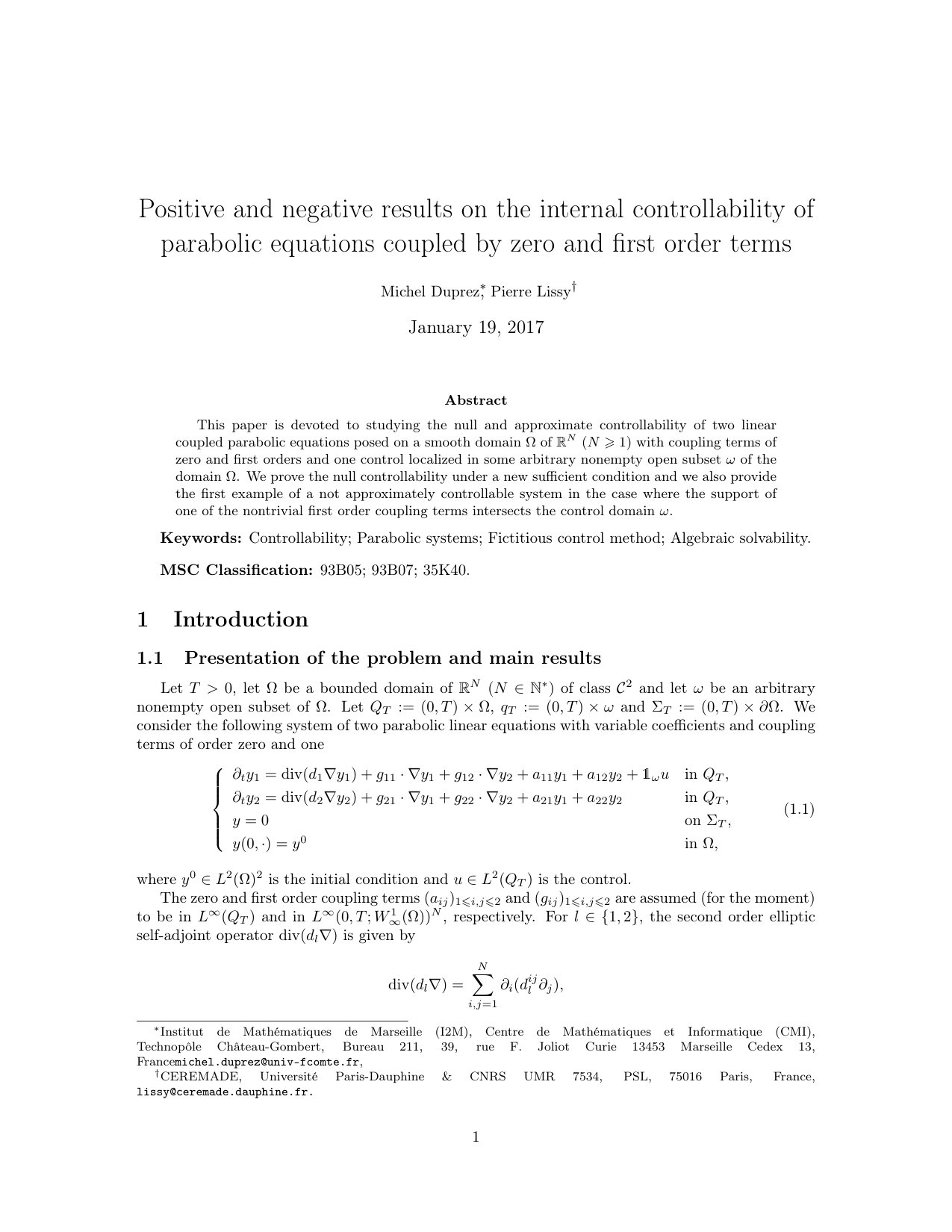 Figure 1
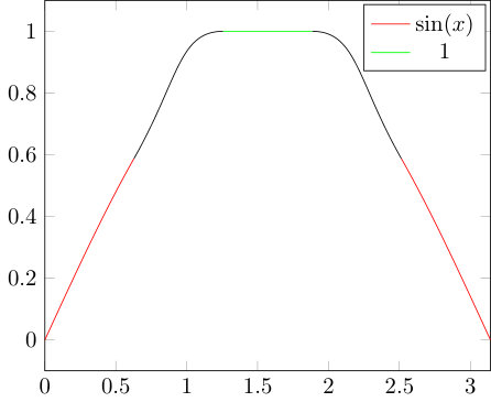 Figure 1
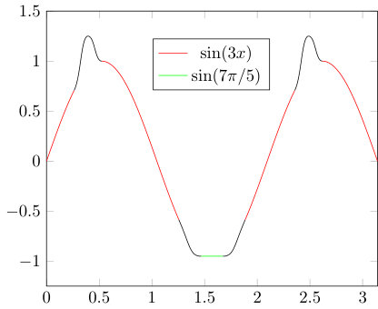 Figure 2
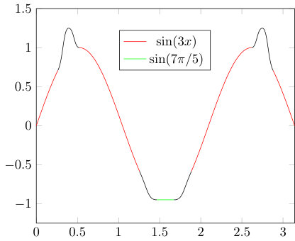 Figure 3
Peer Reviews
No public reviews on file for this paper yet. If you reviewed it on a platform where reviews are public (OpenReview, ICLR, NeurIPS, ICML), you can paste yours below so the community can read it here.
Videos
No videos yet. Explain this paper in a talk, walkthrough, or lecture? Add one.
Positive and negative results on the internal controllability of parabolic equations coupled by zero and first order terms
Michel Duprez*** Institut de Mathématiques de Marseille (I2M), Centre de Mathématiques et Informatique (CMI), Technopôle Château-Gombert, Bureau 211, 39, rue F. Joliot Curie 13453 Marseille Cedex 13, [email protected], , Pierre Lissy†††CEREMADE, Université Paris-Dauphine & CNRS UMR 7534, PSL, 75016 Paris, France, [email protected].
Abstract
This paper is devoted to studying the null and approximate controllability of two linear coupled parabolic equations posed on a smooth domain of () with coupling terms of zero and first orders and one control localized in some arbitrary nonempty open subset of the domain . We prove the null controllability under a new sufficient condition and we also provide the first example of a not approximately controllable system in the case where the support of one of the nontrivial first order coupling terms intersects the control domain .
Keywords: Controllability; Parabolic systems; Fictitious control method; Algebraic solvability.
MSC Classification: 93B05; 93B07; 35K40.
1 Introduction
1.1 Presentation of the problem and main results
Let , let be a bounded domain of () of class and let be an arbitrary nonempty open subset of . Let , and . We consider the following system of two parabolic linear equations with variable coefficients and coupling terms of order zero and one
[TABLE]
where is the initial condition and is the control.
The zero and first order coupling terms and are assumed (for the moment) to be in and in , respectively. For , the second order elliptic self-adjoint operator is given by
[TABLE]
with
[TABLE]
where the coefficients satisfy the uniform ellipticity condition
[TABLE]
for a constant .
It is well-known (see for instance [21, Th. 3, p. 356-358]) that for every initial data and every control , System (1.1) admits a unique solution in , where
[TABLE]
In this article, we are concerned with the approximate or null controllability of System (1.1). Let us recall the precise definitions of these notions. We say that System (1.1) is
approximately controllable on the time interval if for every initial condition , every target and every , there exists a control such that the corresponding solution to System (1.1) satisfies
[TABLE]
null controllable on the time interval if for every initial condition , there exists a control such that the corresponding solution to System (1.1) satisfies
[TABLE]
It is well-known that if a parabolic system like (1.1) is null controllable on the time interval , then it is also approximately controllable on the time interval (this is an easy consequence of usual results of backward uniqueness for parabolic equations as given for example in [11]).
Since the case and in has already been studied in [24], we will always work under the following assumption.
Assumption** 1.1****.**
There exists and a nonempty open subset of such that
[TABLE]
Moreover, as we will see in Section 2, it is possible, with the help of appropriate changes of variables and unknowns (we lose a little bit of regularity on the coefficients though, see Section 2), to replace the coupling operator by the simpler coupling operator (where is the first direction in space), at least locally on some subset of .
Hence, without loss of generality, we can also work under the following assumption.
Assumption** 1.2****.**
There exists a nonempty open subset of such that
[TABLE]
For a nonempty set , let us denote by the subset of composed by the functions depending only on the variables . Let us now introduce the following condition, which will be crucial in our following results, and which is closely related to the particular form for the coupling term given in Assumption 1.2 (removing this assumption would make Condition 1.1 impossible to write down explicitly).
Condition** 1.1****.**
There exists a nonempty open set such that
[TABLE]
where
[TABLE]
Our first main result is the following:
Theorem** 1****.**
Let and for every and . Assume that Assumptions 1.1, 1.2 and Condition 1.1 hold. Then System (1.1) is null controllable at any time .
Remark* 1**.*
Theorem 1 is stated and will be proved in the case of two coupled parabolic equations and one control. However, as in [19], it is possible to extend Theorem 1 to systems of parabolic equations controlled by controls for arbitrary . More precisely, consider the system
[TABLE]
where is the initial data and is the control. Let us suppose that there exists , and a nonempty open subset of such that on . As explained in Section 2, we can suppose that the operator is equal to in . Assume that there exists an open set such that
[TABLE]
where
[TABLE]
Then we can adapt the proof of Theorem 1 to prove that System (1.4) is null controllable on the time interval under suitable regularity conditions on the coefficients.
Remark* 2**.*
Condition 1.1 is clearly technical since it does not even cover the case of constant coefficients proved in [19], the general case given in [12] (under some assumption on the control domain) or the one-dimensional result given in [18]. However, Theorem 3 implies that one cannot expect the null controllability to be true in general without extra assumptions on the coefficients. We do not know what would be a reasonable necessary and sufficient condition on the coupling terms for the null controllability of System (1.1).
The second main result of the present paper is the following surprising result.
Theorem** 2****.**
Let us assume that . Let be a nonempty regular open set satisfying . and consider a function satisfying
[TABLE]
Then there exists such that the system
[TABLE]
is not approximately controllable (hence not null controllable) on the time interval .
In other words, Theorem 2 tells us that for every control set strongly included in , there exists a potential for which approximate controllability of (1.5) does not hold, in any space dimension. We may improve a bit this result on the one-dimensional case, where we are able to obtain the following result, which expresses that for some well-constructed potential , that there exists one control domain on which System (1.6) is not approximately controllable (hence not null controllable) and another control domain on which System (1.6) is null controllable (hence approximatively controllable), highlighting the surprising fact that some geometrical conditions on the control domain has to be imposed in order to obtain a controllability result.
Theorem** 3****.**
Consider the following system
[TABLE]
There exists a coefficient such that:
There exists an open interval such that, for all , System (1.6) is null controllable (then approximatively controllable) at time . 2. 2.
There exists an open interval such that, for all , System (1.6) is not approximatively controllable (then not null controllable) at time .
Remark* 3**.*
Let us mention that Theorems 2 and 3 are the first negative result for the controllability of System (1.1) when the support of the first order coupling term intersects the control domain in the case of distributed controls. The authors want to highlight that the coupling operator is constant in the whole domain and nevertheless the system can be controllable or not following the localisation of the control domain, which is an unexpected phenomenon.
1.2 State of the art
Many models of interest involve (linear or non-linear) coupled equations of parabolic systems, notably in fluid mechanics, medicine, chemistry, ecology, geology, etc., and this explains why during the past years, the study of the controllability properties of linear or nonlinear parabolic systems has been an increasing subject of interest (see for example the survey [7]). The main issue is what is called the indirect controllability, that is to say one wants to control many equations with less controls than equations, by acting indirectly on the equations where no control term appears thanks to the coupling terms appearing in the system. This notion is fondamental for real-life applications, since in some complex systems only some quantities can be effectively controlled. Here, we will concentrate on the previous results concerning the null or approximate controllability of linear parabolic systems with distributed controls, but there are also many other results concerning boundary controls or other classes of systems like hyperbolic systems.
First of all, in the case of zero order coupling terms, the case of constant coefficients is now completely treated and we refer to [5] and [6] for parabolic systems having constant coupling coefficients (with diffusion coefficients that may depend on the space variable though) and for some results in the case of time-dependent coefficients. In the case of zero and one order coupling terms and constant coefficients, a necessary and sufficient condition in the case of equations and controls for constant coefficients is provided in [19] by the authors.
The case of space-varying coefficients remains still widely open despite many new partial results these last years. In the case where the support of the coupling terms intersects the control domain, a general result is proved in [24] for parabolic systems in cascade form with one control force (and possibly one order coupling terms). We also mention [4], where a result of null controllability is proved in the case of a system of two equations with one control force, with an application to the controllability of a nonlinear system of transport-diffusion equations. In the situation where the coupling regions do not intersect the control domain, the situation is still not very well-understood and we have partial results, in general under technical and geometrical restrictions, notably on the control domain (see for example [1], [3], [29] and [8]). Let us mention that in this case, there might appear a minimal time for the null controllability of System (1.1) (see [9]), which is a very surprising phenomenon for parabolic equations, because of the infinite speed of propagation of the information.
Concerning the case of first order coupling terms, we mention [24] which gives some controllability results when the coefficient is equal to zero on the control domain. Let us also mention the recent work [12], which concerns the small systems in small dimension, that is to say and systems. The authors of [12] suppose that the control domain contains a part of the boundary . Recently, in [18], the first author studied a particular cascade system with space dependent coefficients and in dimension one thanks to the moment method, and obtained necessary and sufficient conditions on the coupling terms of order [math] and for the null controllability. To conclude, let us also mention another result given in [19] by the authors, which provides a sufficient condition for null controllability in dimension one for space and time-varying coefficients under some technical conditions on the coefficients, which turns out to be exactly equivalent to Condition 1.1 under Assumption 1.2 (but with more regularity than in Assumption 1.1). Hence, Theorem 1 can be seen as a generalization in the multi-dimensional case of the one-dimensional result given in [19]. For a more detailed state of the art concerning this problem, we refer to [19].
Hence, the present paper improves the previous results in the following sense:
- •
Contrary to [12, 27, 18, 19], we prove in Theorem 1 the null controllability of System (1.1) with a condition on but for space/time dependent coefficients, in any space dimension and without any condition on the control domain.
- •
In the previous results, it was surprising to have some very different sufficient conditions for the null controllability of System (1.1) in the case of first order coupling terms, for example on one hand constant coupling coefficients and on the other hand a region of control which intersects the boundary of the domain. Through the example of a not approximately controllable system given in Theorem 2 and 3, we can now better understand why such different conditions appeared since the expected general condition for the null controllability of System (1.1) with space and time-varying coefficients (i.e. it is sufficient that the control and coupling region intersect) may be false in general if .
2 Simplification of the coupling term
In this section, we will prove that it is possible to replace locally the coupling operator by , where is the first direction in space. This kind of simplification has already been used in [12, Lemma 2.6] for example, and we refer to this article for a more detailed proof (see also [18]). Let us remark that the regularities stated in Lemma 2.1 are higher than the one stated in Theorem 1 due to technical reasons appearing in the proofs of Lemmas 2.1 and 2.2.
Lemma** 2.1****.**
Let for every and . Suppose that Assumption 1.1 is verified. Then, there exist a nonempty open subset of , a positive real number and a -diffeomorphism from to an open set that keeps invariant and such that if we call and , then there exist a matrix , a vector and coefficients such that locally on one has
[TABLE]
**Proof of Lemma 2.1
**Let us consider some open hyper-surface of class included in on which , where is the normalized outward normal on (this can always be done since on and is at least continuous), small enough such that it can be parametrized by a local diffeomorphism
[TABLE]
where is a nonempty open set. We call . Let us consider some extension of (that exists thanks to the regularity of and ) that we denote by . Using the Cauchy-Lipschitz Theorem, we infer that for every , there exists a unique global solution to the Cauchy Problem
[TABLE]
Since is continuous and on , we deduce that there exists some such that for every and every . We define
[TABLE]
Then, by the inverse mapping theorem, is a -diffeomorphism from to with . Let us call and , then it is clear that
[TABLE]
and hence we obtain (2.1) and the regularities wished for the new coefficients by writing down the equation verified by .
Let us now perform a second useful reduction.
Lemma** 2.2****.**
There exists an open subset of and a function such that for some constant and if
[TABLE]
and
[TABLE]
then there exists some coefficients and such that locally on one has
[TABLE]
**Proof of Lemma 2.2
**Let us consider some such that for some constant , and consider the change of unknowns
[TABLE]
Using equation (2.1), we infer that verifies
[TABLE]
where and . Hence, if we choose satisfying and in , which is always possible, then and verify (2.2) and we have and .
3 Proof of Theorem 1
During all this Section, we will always assume that Assumptions 1.1 and 1.2 are satisfied.
3.1 Strategy : Fictitious control method
The fictitious control method has already been used for instance in [25], [17], [2], [16] and [19]. Roughly, the method is the following: we first control the equations with two controls (one on each equation) and we try to eliminate the control on the last equation thanks to algebraic manipulations locally on the control domain. For more details, see for example [19, Section 1.3]. Let us be more precise and decompose the problem into three different steps:
- (i)
**Analytic Problem: Null controllability by two forces
**Find a solution in an appropriate space to the control problem by two controls
[TABLE]
where the controls and are regular enough and with a support strongly included in (remind that was introduced in Condition 1.1). Solving Problem (3.1) is easier than solving the null controllability on the time interval of System (1.1), because we control System (3.1) with one control on each equation. The important point is that the control has to be regular enough, so that it can be differentiated a certain amount of times with respect to the space and/or time variables (see the next section about the algebraic resolution).
Proposition** 3.1****.**
Let . Suppose that and for every and . Then there exists two constants and such that for every initial condition one can find a control verifying moreover for which the solution to System (3.1) is equal to zero at time and the following estimate holds:
[TABLE]
The controllability of parabolic systems with regular controls is nowadays well-known. For a proof of Proposition 3.1, one can adapt the strategy developed in [13, 14, 15, 25] where the authors prove the controllability of parabolic systems with controls thanks to the fictitious control method and the local regularity of parabolic equations. For more details, we refer to [20, Chap. I, Sec. 2.4]. It is also possible to use the Carleman estimates (see for instance [10] and [19, Section 2.3]), however this will impose the coefficients of System (3.1) to be regular in the whole space (and would require higher regularity on ).
- (ii)
**Algebraic Problem: Null controllability by one force
**For given with strictly included in , find , in an appropriate space, satisfying the following control problem:
[TABLE]
with strictly included in , which impose the initial and final data and the boundary conditions. We recall that is equal to in . We will solve this problem using the notion of algebraic resolvability of differential systems, which is based on ideas coming from [26, Section 2.3.8] and was already used in some different contexts in [17], [2], [19] or [16]. The idea is to write System (3.3) as an underdetermined system in the variables and and to see as a source term. More precisely, we remark that System (3.3) can be rewritten as
[TABLE]
where and
[TABLE]
The goal in Section 3.2 will be then to find a partial differential operator satisfying
[TABLE]
Thus to solve control problem (3.3), it suffices to take
[TABLE]
When (3.5) is satisfied, we say that System (3.4) is algebraically solvable.
- (iii)
**Conclusion
**If we are able to solve the analytic and algebraic problems, then it is easy to check that will be a solution to System (1.1) in an appropriate space and will satisfy in (for more explanations, see [17, Prop. 1] and the proof of Theorem 1 on pages 11-12).
3.2 Algebraic solvability of the linear control problem
The goal of this section is to solve algebraic problem (3.4). We will use the following lemma:
Lemma** 3.1****.**
Let be a nonempty open subset of ()* and let . Consider two differential operators and defined for every by*
[TABLE]
where, for , . If for every where
[TABLE]
and is not an element of the -module
[TABLE]
for a nonempty open subset of , then there exists two differential operators and such that
[TABLE]
**Proof of Lemma 3.1
**The goal is to apply some differential operators and to and in order to obtain . So, since is not appearing in , we would like to eliminate all the derivatives in the expression of by differentiations and linear combinations.
If and in for every , we define
[TABLE]
If not, let be the smallest number of such that there exists a nonempty open subset of where . Then we consider the commutator of and :
[TABLE]
Again, if for every , we have in , we define
[TABLE]
If not, let be the smallest number of such that there exists a nonempty open subset of where . Then we consider the commutator of and :
[TABLE]
Again, if, for every , we have in , we define
[TABLE]
If not, we continue the same reasoning that will stop at some point since there is only a finite order of derivatives . Hence, we obtain, for a , a nonempty open subset of and an operator
[TABLE]
Moreover, is obtained by making iterated commutators of operators involving only and . Hence it is clear that there exists two linear partial differential operators and such that
[TABLE]
Hence, in view of (3.8), we will have the desired conclusion as soon as the coefficient in the right-hand side in (3.8) is different from zero. Let us explain into more details what this condition exactly means. For the sake of clarity, let us assume that (but the following reasoning can be extended to any ). We remark that
[TABLE]
holds only if, for some , we have
[TABLE]
The last expression can be rewritten as
[TABLE]
Again, (3.10) holds only if, for some , we have
[TABLE]
or, equivalently,
[TABLE]
Thus (3.9) is satisfied only if, for some , we have
[TABLE]
Hence, we find back condition (1.1) and the proof of Lemma 3.1 is achieved.
We are now able to prove the algebraic solvability of (3.4).
Proposition** 3.2****.**
Suppose that for every and . Then, under Condition 1.1, System (3.4) is algebraically solvable with an operator of order .
**Proof of Proposition 3.2
**Let us remark that the first equation of System (3.4) can be rewritten locally on as
[TABLE]
hence one can always solve algebraically first the second equation of System (3.4), will then be given with respect to , and . Hence, solving (3.4) is equivalent to solving
[TABLE]
where
[TABLE]
Hence, finding a differential operator such that (3.5) is satisfied is now equivalent to finding a differential operator such that
[TABLE]
We can remark that equality (3.12) is formally equivalent to
[TABLE]
where the formal adjoint of the operator is given for every by
[TABLE]
Operator can be rewritten as
[TABLE]
where and are given in (1.3). Let us first consider the following linear combination of and :
[TABLE]
Lemma 3.1 leads to the algebraic resolvability of System (3.4) under Condition 1.1.
Concerning the order of , if we follow the proof of Lemma 3.1 step by step, we apply at most operators of order two to eliminate the terms with (thanks to the symmetry property of ), then at most operators of order one for the term with and finally an operator of order at most one for . Thus the operator is of order at most
We are now ready for the proof of Theorem 1.
**Proof of Theorem 1.
**We apply Proposition 3.1 with and obtain the existence of two constants and such that for every initial condition one can find a control verifying for which the solution to System (3.1) is equal to zero at time and the following estimate holds:
[TABLE]
Now, using Proposition 3.2, locally on there exists a solution to the following control problem:
[TABLE]
with . Moreover, since , we have in .
We conclude by remarking that is a solution to System (1.1) which satisfies in .
4 Proof of Theorem 2
Let be a nonempty regular open set satisfying . Let be a function of satisfying
[TABLE]
Consider the following system
[TABLE]
where is the control and will be specified later. If we can control approximately System (4.1), then it implies that we are also able to control approximately the following equation:
[TABLE]
where is the control. Since on , the approximate controllability on the time interval of System (4.1) is equivalent to the following property, called the Fattorini criterion (see [28, Theorem 1 & Section 3]):
Theorem** 4****.**
System (4.2) is approximately controllable on the time interval , if and only if for every and every , we have
[TABLE]
Since , Then there exists a open set such that . The first eigenfunction of is well-known to be positive in , so we can define a function satisfying
[TABLE]
For instance, if and , as in Figure 1, we may construct a function satisfying
[TABLE]
Consider
[TABLE]
Thanks to the definition of , is well defined in and is an element of . Thus satisfies
[TABLE]
Using Theorem 4, System (4.2) is not approximately controllable on the time interval .
Remark* 4**.*
Let us emphasize that in this case, as expected, Condition 1.1 is not verified: on we have by definition , and for every , which implies that on and , hence
[TABLE]
This will also be the case for the potential constructed in the first part of the proof of Theorem 3.
5 Proof of Theorem 3
Let and . Consider the following system
[TABLE]
where is the control and will be specified later.
As in the previous section, it is well-known that the approximate controllability on the time interval of System (4.2) is equivalent to the following property:
Theorem** 5****.**
System (5.1) is approximately controllable on the time interval , if and only if for every and every , we have
[TABLE]
Let us construct three functions , , satisfying
[TABLE]
The idea will be to construct the function as a perturbation of . Consider a function of satisfying
[TABLE]
where are three nontrivial functions of satisfying
[TABLE]
small enough and are three positive constants to determined (See Figure 2 for some examples of function ). Let us remark that, for a constant to determined, the function defined for all by
[TABLE]
is solution to the first equation of (5.2). In order to apply Theorem 5, let us first prove that and can be chosen such that in . Since in ,
[TABLE]
for all . Since for all in and
[TABLE]
then, according to the last line of (5.3), for small enough, it is possible to choose in order to obtain
[TABLE]
Thus, for given by
[TABLE]
we obtain in . By definition of , we have . Let us now prove that for some appropriate and , we have . We remark that
[TABLE]
Let us distinguish two cases:
If
[TABLE]
is negative, then, using the fact that for all , one can choose and find some some such that . 2. 2.
If now the quantity (5.5) is positive, since and for all , one can choose and find some some such that .
The function will have one of the two following forms
To satisfy the second equality in (5.2), we define the function as follows
[TABLE]
This function is bounded since at each point where is null, i.e. at [math], , and , there exists a neighbourhood in which is equal to . Thus the constructed , and verify (5.2). Using Theorem 5, System (5.1) is not approximately controllable on the time interval .
Let us now prove the second item of Theorem 3. We remark that it is possible to chose in with small enough. Then is defined in for all by
[TABLE]
Thus satisfies Condition 1.1 for , that is is non-constant in the space variable on . We conclude applying Theorem 1 for .
Funding
Pierre Lissy is partially supported by the project IFSMACS funded by the french Agence Nationale de la Recherche, 2015-2019 (Reference: ANR-15-CE40-0010).
Conflict of Interest
The authors declare that they have no conflict of interest.
The reference list from the paper itself. Each links out to its DOI / PubMed record.
- 1[1] F. Alabau-Boussouira. A hierarchic multi-level energy method for the control of bidiagonal and mixed n 𝑛 n -coupled cascade systems of PDE’s by a reduced number of controls. Adv. Differential Equations , 18(11-12):1005–1072, 2013.
- 2[2] F. Alabau-Boussouira, J.-M. Coron, and G. Olive. Internal controllability of first order quasilinear hyperbolic systems with a reduced number of controls,. Submitted , 2015.
- 3[3] F. Alabau-Boussouira and M. Léautaud. Indirect controllability of locally coupled wave-type systems and applications. J. Math. Pures Appl. (9) , 99(5):544–576, 2013.
- 4[4] F. Ammar Khodja, A. Benabdallah, and C. Dupaix. Null-controllability of some reaction-diffusion systems with one control force. J. Math. Anal. Appl. , 320(2):928–943, 2006.
- 5[5] F. Ammar Khodja, A. Benabdallah, C. Dupaix, and M. González-Burgos. A generalization of the Kalman rank condition for time-dependent coupled linear parabolic systems. Differ. Equ. Appl. , 1(3):427–457, 2009.
- 6[6] F. Ammar Khodja, A. Benabdallah, C. Dupaix, and M. González-Burgos. A Kalman rank condition for the localized distributed controllability of a class of linear parbolic systems. J. Evol. Equ. , 9(2):267–291, 2009.
- 7[7] F. Ammar Khodja, A. Benabdallah, M. González-Burgos, and L. de Teresa. Recent results on the controllability of linear coupled parabolic problems: a survey. Math. Control Relat. Fields , 1(3):267–306, 2011.
- 8[8] F. Ammar Khodja, A. Benabdallah, M. González-Burgos, and L. de Teresa. Minimal time of controllability of two parabolic equations with disjoint control and coupling domains. C. R. Math. Acad. Sci. Paris , 352(5):391–396, 2014.