Calculation of Relativistic Nucleon-Nucleon Potentials in Three-Dimensions
M. R. Hadizadeh, M. Radin
TL;DR
This paper develops a three-dimensional method to calculate relativistic nucleon-nucleon potentials, accurately relating relativistic and non-relativistic interactions through integral equations and numerical solutions.
Contribution
It introduces a novel three-dimensional approach for deriving relativistic nucleon-nucleon potentials from non-relativistic ones, using integral equations and iterative numerical methods.
Findings
Relativistic potentials preserve two-nucleon observables with high accuracy.
The method effectively relates relativistic and non-relativistic interactions.
Numerical tests confirm the approach's validity.
Abstract
In this paper, we have applied a three-dimensional approach for calculation of the relativistic nucleon-nucleon potential. The quadratic operator relation between the non-relativistic and the relativistic nucleon-nucleon interactions is formulated as a function of relative two-nucleon momentum vectors, which leads to a three-dimensional integral equation. The integral equation is solved by the iteration method, and the matrix elements of the relativistic potential are calculated from non-relativistic ones. Spin-independent Malfliet-Tjon potential is employed in the numerical calculations, and the numerical tests indicate that the two-nucleon observables calculated by the relativistic potential are preserved with high accuracy.
Click any figure to enlarge with its caption.
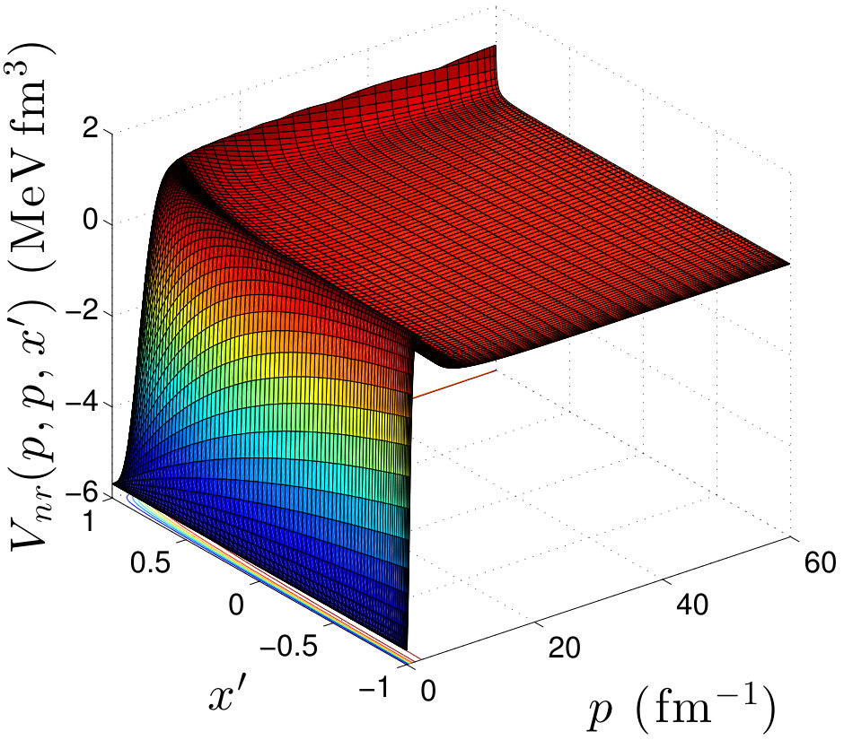 Figure 1
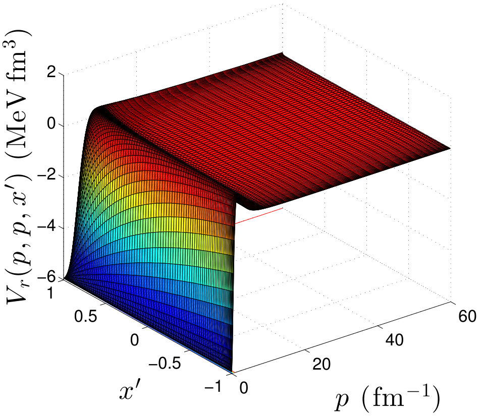 Figure 2
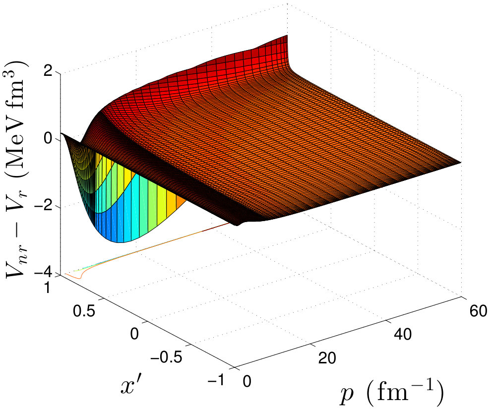 Figure 3
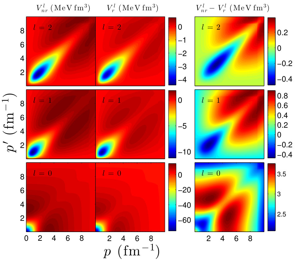 Figure 4
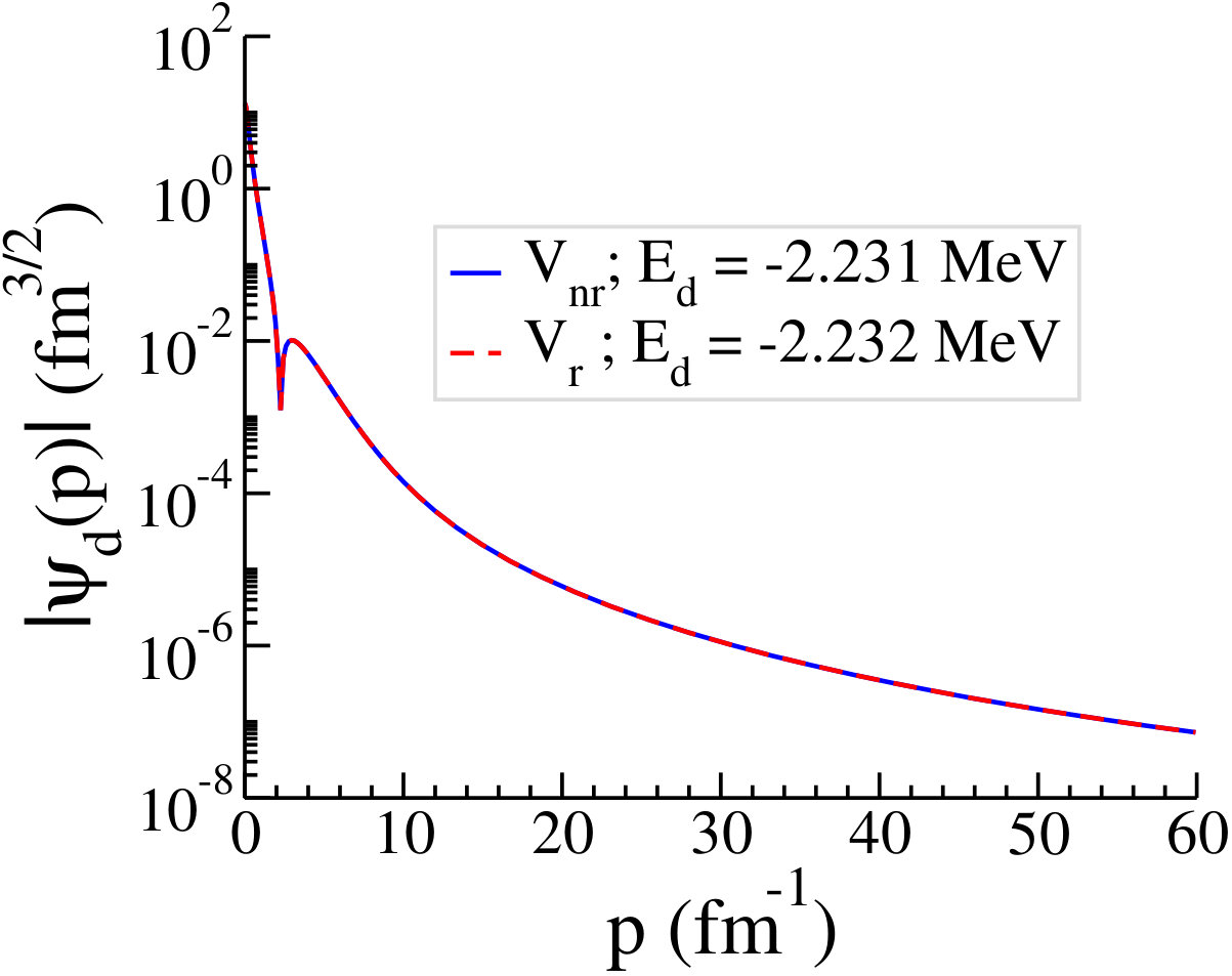 Figure 5
| -626.8932 | 1.550 | 1438.7228 | 3.11 |
| 1 | 0 | 17 |
| 1 | 1 | 18 |
| 2 | 1 | 12 |
| 3 | 1 | 10 |
| 4 | 1 | 8 |
| 5 | 1 | 10 |
| 1.1099096 | 0.7084511 | -1.6327025 | |
|---|---|---|---|
| Iteration # | |||
| 0 | 1.0525724 | 0.6718530 | -1.5483583 |
| 1 | 0.7838006 | 0.3920976 | -1.8512322 |
| 2 | 0.8895160 | 0.4979858 | -1.7453002 |
| 3 | 0.8853336 | 0.4938142 | -1.7495059 |
| 4 | 0.8848131 | 0.4932883 | -1.7500527 |
| 5 | 0.8847858 | 0.4932573 | -1.7500929 |
| 6 | 0.8847910 | 0.4932608 | -1.7500930 |
| 7 | 0.8847932 | 0.4932623 | -1.7500928 |
| 8 | 0.8847938 | 0.4932626 | -1.7500930 |
| 9 | 0.8847939 | 0.4932626 | -1.7500931 |
| 10 | 0.8847939 | 0.4932626 | -1.7500932 |
| 11 | 0.8847939 | 0.4932626 | -1.7500933 |
| 12 | 0.8847939 | 0.4932626 | -1.7500933 |
| (MeV) | (MeV) | |
|---|---|---|
| -2.23100 | -2.23229 | 0.05782 |
| (MeV) | (mb) | (mb) | |
|---|---|---|---|
| 1 | 15274.4 | 15273.3 | 0.00720 |
| 10 | 14526.4 | 14525.5 | 0.00620 |
| 25 | 11485.5 | 11484.9 | 0.00522 |
| 50 | 6367.46 | 6367.31 | 0.00236 |
| 75 | 3432.10 | 3432.08 | 0.00058 |
| 100 | 1926.16 | 1926.17 | 0.00052 |
| 200 | 297.580 | 297.586 | 0.00202 |
| 300 | 129.008 | 129.015 | 0.00543 |
| 400 | 94.6592 | 94.6631 | 0.00412 |
| 500 | 72.6167 | 72.6201 | 0.00468 |
| 600 | 56.9070 | 56.9111 | 0.00720 |
| (MeV) | |||
|---|---|---|---|
| 1 | 178.399202 | 178.399259 | 0.00003 |
| 10 | 164.191097 | 164.191642 | 0.00033 |
| 25 | 142.727577 | 142.728682 | 0.00077 |
| 50 | 115.599510 | 115.600883 | 0.00119 |
| 75 | 96.723079 | 96.724553 | 0.00152 |
| 100 | 82.604149 | 82.605322 | 0.00142 |
| 200 | 46.516325 | 46.517103 | 0.00167 |
| 300 | 24.195385 | 24.196576 | 0.00492 |
| 400 | 8.220831 | 8.220032 | 0.00972 |
| 500 | 176.141274 | 176.139179 | 0.00119 |
| 600 | 166.764703 | 166.759452 | 0.00315 |
| (MeV) | |||
| 1 | 0.000015228 | 0.000015228 | 0.0017533 |
| 10 | 0.01.520323 | 0.015203706 | 0.0030894 |
| 25 | 0.235486179 | 0.235489846 | 0.0015574 |
| 50 | 1.820265835 | 1.820327160 | 0.0033690 |
| 75 | 5.735591957 | 5.735736050 | 0.0025123 |
| 100 | 12.07379026 | 12.07410200 | 0.0025819 |
| 200 | 35.51818548 | 35.51899747 | 0.0022861 |
| 300 | 36.92310114 | 36.92426648 | 0.0031561 |
| 400 | 31.28393516 | 31.28424025 | 0.0009752 |
| 500 | 24.51728521 | 24.51716984 | 0.0004706 |
| 600 | 18.01488447 | 18.01311044 | 0.0098475 |
Peer Reviews
No public reviews on file for this paper yet. If you reviewed it on a platform where reviews are public (OpenReview, ICLR, NeurIPS, ICML), you can paste yours below so the community can read it here.
Videos
No videos yet. Explain this paper in a talk, walkthrough, or lecture? Add one.
11institutetext: Institute of Nuclear and Particle Physics and Department of Physics and Astronomy, Ohio University, Athens, OH 45701, USA, 22institutetext: College of Science and Engineering, Central State University, Wilberforce, OH 45384, USA, 33institutetext: Department of Physics, K. N. Toosi University of Technology, P.O.Box 16315–1618, Tehran, Iran.
Calculation of Relativistic Nucleon-Nucleon Potentials in Three-Dimensions
M. R. Hadizadeh [email protected]
M. Radin [email protected]
(Received: date / Revised version: date)
Abstract
In this paper, we have applied a three-dimensional approach for calculation of the relativistic nucleon-nucleon potential. The quadratic operator relation between the non-relativistic and the relativistic nucleon-nucleon interactions is formulated as a function of relative two-nucleon momentum vectors, which leads to a three-dimensional integral equation. The integral equation is solved by the iteration method, and the matrix elements of the relativistic potential are calculated from non-relativistic ones. Spin-independent Malfliet-Tjon potential is employed in the numerical calculations, and the numerical tests indicate that the two-nucleon observables calculated by the relativistic potential are preserved with high accuracy.
pacs:
21.45-vFew-body systems and 21.45.BcTwo-nucleon system and 24.10.JvRelativistic models
1 Introduction
The inputs for the relativistic three-body (3B) bound and scattering state calculations Witala_PRC83 -Kamada_MPLA24 are the fully off–shell relativistic nucleon–nucleon () matrices, which can be obtained by solving the relativistic Lippmann–Schwinger (LS) integral equation using relativistic interactions.
It is known that there is a nonlinear operator relation between the non-relativistic and the relativistic interactions. So, the first step toward the calculation of relativistic matrices is the calculation of the relativistic potentials from non-relativistic ones. To this aim, the matrix elements of the relativistic potential in momentum space are traditionally calculated by solving the nonlinear equation using the following different methods.
In the spectral expansion method, the quadratic equation is solved by inserting a completeness relation of the bound and scattering states into the right side of the quadratic equation and by projecting the result into the momentum space Kamada_PRC66 ; Gloeckle_PRC33 . So, by having the non-relativistic potential one can first calculate the bound state wave function and scattering half-shell matrix and used the result to solve the nonlinear equation.
In the iteration method, the nonlinear equation is solved by iteration. Kamada and Glöckle introduced a powerful numerical technique to calculate the matrix elements of the relativistic potential directly from the matrix elements of the non-relativistic potential Kamada_PLB655 . In this method, the nonlinear integral equation is solved using the iteration method to get relativistic and boosted potentials from non-relativistic ones. It is successfully implemented in the problem, but it has not yet been extended to a three-dimensional (3D) approach.
Another method is to multiply the non-relativistic potential by a function that depends on relative momenta, in such a way that both the non-relativistic and the relativistic potentials leads to same phase shifts and observables Kamada_MPLA80 . The function is defined in such a way that it changes the non-relativistic kinetic energy to relativistic kinetic energy by rescaling the momentum variables, which leads to the same binding energy for both non-relativistic and relativistic potentials.
In the past decade a 3D approach based on momentum vector variables was developed to study the few–body bound and scattering problems Hadizadeh_EPJC113_rel -Fachruddin_PRC63 . In the 3D approach one works directly with vector variables which lead to 3D integral equations, whereas the partial wave (PW) representation in the angular momentum basis leads to coupled equations. In the PW representation, depending on the energy scale of the problem, one must sum PWs, and consequently at higher energies one needs to consider a larger number of PWs, however the 3D approach automatically contains all PWs and the number of equations is energy independent.
We would like to point out that as Polyzou and Elster have shown one can directly calculate the relativistic matrix from the non-relativistic one, without needing to solve the nonlinear equation. Consequently, one does not need to solve the LS equation for the embedded interaction, and one can calculate the fully off-shell relativistic matrix by following a two-step process. The first step is to obtain the relativistic right–half–shell (RHS) matrix from the non-relativistic RHS matrix by an analytical relation proposed by Coester et al. Coester . The second step is to calculate the fully–off–shell matrix from the RHS matrix by solving a first resolvent equation. Keister et al. Keister proposed the method and it is implemented for the first time in a 3B scattering calculation Lin_PRC76 in this way. Using the direct calculation of the relativistic matrix from the non-relativistic one, recently the relativistic effects were studied in the 3B binding energy using a 3D scheme Hadizadeh_EPJC113_rel ; Hadizadeh_PRC90 . The relativistic 3B wave function was calculated for the first time, and it was shown that the relativistic effects lead to a reduction of about 3% in the 3B binding energy for two models of a spin-independent Malfliet-Tjon type potential. Since the 3D approach automatically considers all PWs, if it works for the bound state, it can also be extended to the scattering problem, independent of the range of energy. The next step is to consider the spin and isospin degrees of freedom and work with realistic interactions.
In this work, we have applied the iteration method proposed by Kamada and Glöckle to construct the relativistic potential from the non-relativistic Malfliet–Tjon potential in a 3D scheme, without using the PW decomposition.
2 Three-dimensional formulation of the quadratic operator relation between the relativistic and non-relativistic potentials
According to Bakamjian and Thomas Bakamjian_PR92 and Fong and Sucher Fong_JMP5 , the relativistic dynamics is specified in terms of the mass operator
[TABLE]
where , is the mass of the nucleons and is the relative momentum of two nucleons. The connection between the relativistic and non-relativistic potentials, i.e. and , is defined by the quadratic operator equation Kamada_PLB655
[TABLE]
The matrix elements of the relativistic potential can be obtained from the non-relativistic potentials by the projection of Eq. (2) into the basis states
[TABLE]
In our study we have followed Kamada and Glöckle’s strategy Kamada_PLB655 to obtain the matrix elements of the relativistic potential, i.e. , directly from the non-relativistic one, i.e. without using PW decomposition. Here we discuss the numerical solution of Eq. (2) as a function of the magnitude of the momentum vectors and the angle between them. In our calculations we have used the spin independent Malfliet–Tjon (MT) potential, which is a superposition of short–range repulsive and long–range attractive Yukawa interactions Malfliet
[TABLE]
where . The parameters of the MT–I potential are given in Table 1. In order to obtain the matrix elements of therelativistic potential, we have solved Eq. (2) by the iteration method. A coordinate system is defined by choosing the relative momentum vector parallel to axis and vector in the plane, so that Eq. (2) can be written explicitly as
[TABLE]
where
[TABLE]
We start the iteration with
[TABLE]
and stop it when the calculated relativistic potential satisfies Eq. (5) with a relative error of at each set point . To speed up the convergence procedure in solving Eq. (5) we can redefine the relativistic potential in each step of the iteration as a linear combination of the calculated relativistic potential in the last two successive iterations as
[TABLE]
Kamada and Glöckle have used in their calculations for the AV18 potential. Our numerical analysis shows that the larger values of can lead to faster convergence in the solution of Eq. (5). In Table 2 we have shown the number of iterations to reach convergence in Eq. (5) for different values of and . It indicates that and leads to faster convergence for the calculation of the relativistic potential from the MT–I bare potential.
For the discretization of the continuous momentum and angle variables we used the Gauss-Legendre quadrature. For the momentum variables a hyperbolic plus linear mapping is used to cover the integration domain by the subintervals
[TABLE]
The typical values for , and are , and fm*-1* respectively. In our calculations we have used mesh points for the momentum variables, mesh points for the spherical and mesh points for the azimuthal angle variables. In each iteration we needed to interpolate on the angle variable and to avoid extrapolation we have added the extra points to the angle mesh points . In order to save run time and memory in solution of equation (5) we have used the symmetry property of the kernel to calculate the integration over azimuthal angle on the domain
[TABLE]
In Figs. 1 and 2 we have shown our numerical results for the relativistic potential calculated from the MT–I potential. The bare MT–I potential as well as the difference between the bare and constructed relativistic potentials is also shown. The plots of Fig. 1 show the non-relativistic and relativistic potentials as well as their difference as a function of the relative momenta and the angle between them . It seems the solution of the quadratic equation for the relativistic potential completely changes the structure of the potential at forward angles for diagonal matrix elements , and the relativistic potential is almost smooth in comparison with the non-relativistic potential. The corresponding plots in Fig. 2, show the partial wave projection of the non-relativistic and the relativistic potentials and also their differences, calculated from the 3D representation by , as a function of the relative momenta and . As we can see the matrix elements of the relativistic and non-relativistic potentials are larger for the lower partial waves and consequently their differences become higher.
Table 3 shows an example of the convergence of the matrix elements of the relativistic potential by iteration number for the fixed points ( fm*-1*, fm*-1*, ) for and .
3 Numerical tests of the relativistic potential
3.1 bound state
The total Hamiltonian of two interacting nucleons in the center of mass system is:
[TABLE]
where is the free Hamiltonian, is the non-relativistic interaction and is the initial (final) relative momentum of two nucleons. The Lippmann–Schwinger equation for the two–nucleon bound state is given as
[TABLE]
which can be represented in momentum space as the following eigenvalue equation
[TABLE]
The relativistic Schrödinger equation for the two–nucleon bound state has the form
[TABLE]
where is the deuteron mass. The relativistic deuteron wave function satisfies the eigenvalue equation
[TABLE]
Our numerical results for the deuteron binding energy and wave function calculated by relativistic and non-relativistic potentials are given in Table 4 and Fig. 3. As we can see the constructed relativistic potential preserves the deuteron binding energy obtained by the bare MT–I potential with high accuracy and the relative percentage difference of about .
3.2 scattering
The inhomogeneous Lippmann–Schwinger equation which describes two–nucleon scattering can be represented in momentum space as
[TABLE]
The differential cross section for elastic scattering as a function of incident projectile energy is given by
[TABLE]
where
[TABLE]
Consequently, the total cross section can be obtained directly from the differential cross section as
[TABLE]
The relativistic scattering can be described by the relativistic form of the Lippmann–Schwinger equation as
[TABLE]
The relativistic differential and total cross sections can be obtained by Eqs. (18) and (20) and by replacing with .
In Table 5, our numerical results for the total elastic scattering cross sections obtained by the constructed relativistic potential from the MT–I potential are given as a function of the on–shell momentum . As we can see the relativistic total cross sections are in excellent agreement with the corresponding non-relativistic cross sections and have a percentage relative difference of less than . phase shifts in the PW scheme are calculated by
[TABLE]
where the partial wave matrix, i.e. , can be obtained from the 3D form of the matrix, i.e. , as
[TABLE]
In Table 6, we have shown our numerical results for the and wave phase shifts as a function of the on–shell momentum calculated from the projection of the 3D form of the non-relativistic and relativistic matrices by Eq. (30). As we can see the relativistic and wave phase shifts are in excellent agreement with the corresponding non-relativistic ones and have a relative percentage difference of less than and respectively.
4 Discussion and outlook
In this paper, we have used a three-dimensional approach to formulating the relativistic nucleon-nucleon potential as a function of the two-body relative momentum vectors. The quadratic equation which connects the relativistic and non-relativistic nucleon-nucleon interactions is presented in momentum space as a three-dimensional integral equation. For the first numerical implementation, the integral equation is solved by the spin-independent Malfliet-Tjon potential, and the matrix elements of the relativistic potential are calculated as a function of the two-body relative momenta and the angle between them. Our numerical analysis confirms that the two-body observables calculated from the relativistic potential are preserved. The extension of this formalism to realistic nucleon-nucleon interactions with spin degrees of freedom in a momentum-helicity basis state is currently underway.
Acknowledgements
We thank Professor Hiroyuki Kamada for helpful discussions and also thank Dr. Jeremy Holtgrave for reading the manuscript in detail and suggesting substantial improvements. This work is performed under the auspices of the National Science Foundation under Contract No. NSF-HRD-1436702 with Central State University. M. R. H. acknowledges the partial support from the Institute of Nuclear and Particle Physics at Ohio University.
The reference list from the paper itself. Each links out to its DOI / PubMed record.
- 1(1) H. Witała, J. Golak, R. Skibiński, W. Glöckle, H. Kamada, and W.N. Polyzou, Phys. Rev. C 83 , 044001 (2011); Phys. Rev. C 88 (E), 069904 (2013).
- 2(2) H. Witała, J. Golak, R. Skibiński, W. Glöckle, W. N. Polyzou, and H. Kamada, Phys. Rev. C 77 , 034004 (2008).
- 3(3) K. Sekiguchi et al., Phys. Rev. Lett. 95 , 162301 (2005).
- 4(4) H. Witała, J. Golak, W. Glöckle, and H. Kamada, Phys. Rev. C 71 , 054001 (2005).
- 5(5) H. Witała, J. Golak, R. Skibiński, W. Glöckle, W. Polyzou, and H. Kamada, Few-Body Syst. 49 , 61(2011).
- 6(6) T. Lin, Ch. Elster, W. N. Polyzou, and W. Glöckle, Phys. Lett. B 660 , 345 (2008).
- 7(7) T. Lin, Ch. Elster, W. N. Polyzou, and W. Glöckle, Phys. Rev. C 76 , 014010 (2007).
- 8(8) H. Witała, J. Golak, R. Skibnski, W. Glöckle, W. N. Polyzou, and H. Kamada, Mod. Phys. Lett. A 24 , 871 (2009).