Specht Polytopes and Specht Matroids
John D. Wiltshire-Gordon, Alexander Woo, and Magdalena Zajaczkowska

TL;DR
This paper introduces Specht matroids and polytopes to capture relations in Specht modules, extends the concept to Kronecker coefficients, and provides computational tools, offering new geometric perspectives in representation theory.
Contribution
It defines Specht and Kronecker matroids and polytopes, introduces the concept of matroidification, and supplies computational code for these structures.
Findings
Symmetric group acts transitively on Specht polytope vertices.
Specht polytope's ambient space is irreducible under group action.
Provides elementary construction of Specht modules and computational tools.
Abstract
The generators of the classical Specht module satisfy intricate relations. We introduce the Specht matroid, which keeps track of these relations, and the Specht polytope, which also keeps track of convexity relations. We establish basic facts about the Specht polytope, for example, that the symmetric group acts transitively on its vertices and irreducibly on its ambient real vector space. A similar construction builds a matroid and polytope for a tensor product of Specht modules, giving "Kronecker matroids" and "Kronecker polytopes" instead of the usual Kronecker coefficients. We dub this process of upgrading numbers to matroids and polytopes "matroidification," giving two more examples. In the course of describing these objects, we also give an elementary account of the construction of Specht modules different from the standard one. Finally, we provide code to compute with Specht…
Click any figure to enlarge with its caption.
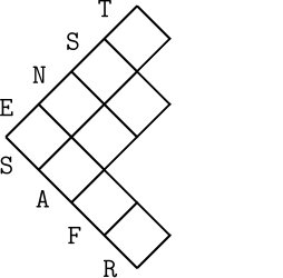 Figure 1
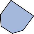 Figure 2
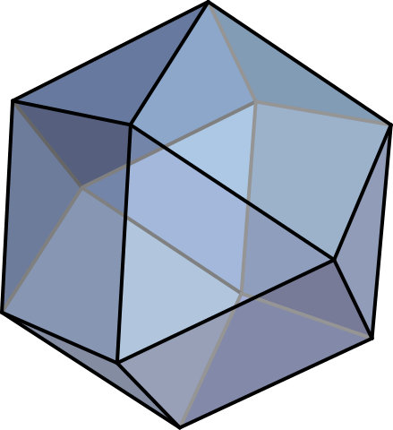 Figure 3
 Figure 4
Peer Reviews
No public reviews on file for this paper yet. If you reviewed it on a platform where reviews are public (OpenReview, ICLR, NeurIPS, ICML), you can paste yours below so the community can read it here.
Videos
No videos yet. Explain this paper in a talk, walkthrough, or lecture? Add one.
Taxonomy
TopicsAdvanced Topics in Algebra · Advanced Combinatorial Mathematics · Algebraic structures and combinatorial models
∎
11institutetext: John D. Wiltshire-Gordon 22institutetext: University of Wisconsin, Madison; Department of Mathematics; Van Vleck Hall; 480 Lincoln Drive; Madison, WI 53706; USA, 22email: [email protected]
Alexander Woo 33institutetext: University of Idaho; Department of Mathematics; University of Idaho; 875 Perimeter Drive MS 1103; Moscow, ID 83844; USA, 33email: [email protected]
Magdalena Zajaczkowska 44institutetext: University of Warwick; Mathematics Institute; Gibbet Hill Rd; Coventry CV4 7AL; UK, 44email: [email protected]
Specht Polytopes and Specht Matroids
John D. Wiltshire-Gordon
Alexander Woo
and Magdalena Zajaczkowska
Abstract
The generators of the classical Specht module satisfy intricate relations. We introduce the Specht matroid, which keeps track of these relations, and the Specht polytope, which also keeps track of convexity relations. We establish basic facts about the Specht polytope, for example, that the symmetric group acts transitively on its vertices and irreducibly on its ambient real vector space. A similar construction builds a matroid and polytope for a tensor product of Specht modules, giving “Kronecker matroids” and “Kronecker polytopes” instead of the usual Kronecker coefficients. We dub this process of upgrading numbers to matroids and polytopes “matroidification,” giving two more examples. In the course of describing these objects, we also give an elementary account of the construction of Specht modules different from the standard one. Finally, we provide code to compute with Specht matroids and their Chow rings.
The irreducible representations of the symmetric group were worked out by Young and Specht in the early 20th century, and they remain omnipresent in algebraic combinatorics. The symmetric group has a unique irreducible representation for each partition of . For example, has exactly five irreducible representations corresponding to the partitions
[TABLE]
Young and Specht constructed these irreducible representations, which are now called Specht modules. Young Young gave a matrix representation and Specht Specht gave a combinatorial spanning set. Garnir Garnir later explained how to rewrite Specht’s spanning set in terms of Young’s basis. These rewriting rules are now called Garnir relations. Modern accounts of these constructions can be found in Sagan Sagan or James and Kerber JK .
This classical approach, however, privileges Young’s basis over other bases and the Garnir relations over other linear dependencies. Focusing on Young’s basis and the Garnir relations immediately breaks the symmetry of Specht’s spanning set and ignores its other combinatorial properties. Certainly, there are linear relations other than those given by Garnir and bases other than those given by Young to investigate!
To this end, we introduce the Specht matroid, which encodes all the linear dependencies among the vectors of Specht’s spanning set. We also introduce the Specht polytope, which provides a way to visualize the Specht module, since the polytope sits inside the corresponding real vector space with positive volume, and the action of the symmetric group takes the polytope to itself.
In the case of the partition , we recover both classical constructions and objects of current research interest. The corresponding Specht polytope is essentially the root polytope of type . In Theorem 6.2, we record a result of Ardila, Beck, Hosten, Pfeifle and Seashore ABHPS describing the faces of this polytope. The Specht matroid for the partition is the matroid of the braid arrangement, and hence its Chow ring is the cohomology ring for the moduli space of marked points on the complex projective line DP ; FY .
We compute further examples of Chow rings in §4, including the solution to Problem 1 on Grassmannians in Sturmfels , which partially inspired this project. We state a combinatorial conjecture for the graded dimensions of the Chow rings for the Specht matroid for the partition . However, we do not study any further connections with moduli spaces.
Our approach allows us to upgrade familiar combinatorial coefficients to matroids and polytopes. By analogy with categorification, which sometimes upgrades numbers to vector spaces, we call this process matroidification, or polytopification when working over the reals. This is the subject of Section 7. In Theorem 7.1, we polytopify the Kronecker coefficients, building the Kronecker polytopes. We also construct the Kronecker matroids encoding the Garnir-style rewriting rules that govern linear dependence in a tensor product of Specht modules. An analogue of Young’s basis for the Kronecker matroid would provide a combinatorial rule for computing Kronecker coefficients. In Theorems 7.2 and 7.3, we give similar results for Littlewood-Richardson coefficients and plethysm coefficients.
The outline of the article is as follows. We begin in Section 1 with a self-contained construction of the Specht module that is suited to our purposes. This construction is a bit unusual in that it makes no mention of tabloids, polytabloids, standard tableaux, or the group algebra. In Sections 3, 4, and 5, we introduce respectively the Specht matroid, its Chow ring, and the Specht polytope; we then prove some basic general facts about them. Section 6 is devoted to the partitions and , for which the Specht matroids and polytopes coincide with other well-studied objects. We describe Kronecker, Littlewood–Richardson, and plethysm matroids and polytopes in Section 7. Section 8 includes code for calculating the objects described in this paper.
1 Introduction to Specht Modules
Our aim in this section is to give an exposition of the representation theory of the symmetric group that is motivated from elementary combinatorial considerations. The reader who wishes to start with the main statements should first look at Definitions 11 and 12 and Theorem 1.2.
We begin with an elementary combinatorics problem: In how many distinct ways can the letters in a word TENNESSEE be rearranged? There are ways to move the letters around, but since some letters are repeated, some of these rearrangements give the same string. For example, the four Es can be rearranged to appear in any order without affecting the string. This reasoning gives the following answer:
[TABLE]
The idea of rearranging letters can be formalized as an action of the symmetric group. In our example acts on the word TENNESSEE. The stabilizer subgroup of with respect to the word TENNESSEE is isomorphic to . Hence the previous argument actually provides an isomorphism of -sets, which is to say, a bijection that commutes with the group action:
[TABLE]
Using the orbit-stabilizer theorem, we recover the numerical answer above.
Now we add a layer of complexity. Suppose we wish to understand the -set
[TABLE]
where acts diagonally (i.e. simultaneously) on the two factors. This diagonal action makes sense because SASSAFRAS has the same number of letters as TENNESSEE. Each factor in this Cartesian product has a single -orbit, but the product certainly does not! For example, the pairs
[TABLE]
cannot be in the same orbit because the upper Es and lower Ss always appear together in the first pair but not in the second. Another proof is that their orbits have different sizes. Indeed, if we consider a column such as as a compound letter, then the total number of distinct rearrangements of the first compound word in these compound letters is , which does not equal the number of rearrangements of the second compound word.
For the construction of the Specht module, we are interested in free orbits. (Recall that an orbit is free if each of its points has trivial stabilizer.) In our context, a non-trivial stabilizer comes from repeated columns. So a pair is in a free orbit if and only if all of its columns are distinct. For example,
[TABLE]
has no repeated columns, so its orbit is free. We claim:
- •
there is only one free orbit, and therefore,
- •
we have already found it.
- •
The proof is basically a picture, and even better,
- •
the proof-picture-idea is strong enough to construct a complete set of irreducible representations over for the symmetric group . These are the Specht Modules. (The story would be the same for any field of characteristic zero.)
Here is the picture.
The boxes provide a simultaneous histogram tallying the letter multiplicities for each word. From the picture, we see that the letter E from the word TENNESSEE must appear once with each of the letters S, A, F, and R. Indeed, in order to keep distinct the four columns in which E appears, E must be paired with each of the four available letters in the bottom row.
Removing the four Es from the pool along with one copy of each of the letters S, A, F, and R, we may proceed to pair off N with the two letters S and A. Continuing inductively, we see that the combinations that appear in a valid pair of rearrangements give the boxes in the diagram.
We give some definitions that encode these pictures.
Definition 1
A partition of is an integer vector such that with . The number is the length of the partition.
Definition 2
A diagram is a finite subset of . The elements of a diagram are called boxes.
Definition 3
Given a partition , the diagram associated to is
[TABLE]
where, by convention, if .
The partition in our running example is ; its associated diagram is
[TABLE]
Here and everywhere else, we will use matrix coordinates, so denotes the box in the second row and third column.
The following proposition is immediate.
Proposition 1
A diagram is the diagram of some partition if and only if is closed under coordinate-wise . In other words, for some if and only if, for any and any with and , .
Definition 4
We say two words of (the same) length have complementary rearrangements if the diagonal action of on the product
[TABLE]
has a unique free orbit. If, furthermore, is in this free orbit, then we say and are complementary.
For example, our diagram above shows that TENNESSEE and SASSAFRAS have complementary rearrangements. The two words are not complementary, but TENENEESS and SASSAFRAS are complementary.
Theorem 1.1
Two words have complementary rearrangements if and only if there exists a parititon diagram with the “simultaneous histogram” property
[TABLE]
Proof
We have already argued the hard direction. If we have a partition diagram with the simultaneous histogram property, we can put in the box the -th most common letter in and the -th most common letter in (breaking ties arbitrarily). The boxes have distinct pairs, so there exists at least one free orbit; this orbit is unique by the iterative argument below Figure 1. In the other direction, rewrite the words using numbers in so that (in each word) appears at least as often as . Then take
[TABLE]
∎
We will proceed to use the idea of complementary words to construct irreducible representations of the symmetric group . Before doing so, we recall some basic definitions in representation theory.
Definition 5
Let be a group. A (complex) representation of is a -vector space along with a linear action of on , meaning that, for any vectors , any scalar , and any group element ,
- •
, and
- •
.
Alternatively, the data of a representation can be encoded in a group homomorphism , where is the group of invertible linear automorphisms of .
Definition 6
If and are representations of , a linear transformation is a map of representations if commutes with the action of , meaning that for all and all .
Definition 7
If and are representations of , then the tensor product is a representation of under the action
[TABLE]
Definition 8
If is a representation of , then is a representation of under the action where, for and , is the functional defined by
[TABLE]
for any .
We need two definitions specific to the group .
Definition 9
For any , the representation is the one dimensional vector space on which acts by sign. This means, for , if is an even permutation and if is an odd permutation.
If is any representation of , then is isomorphic to as a vector space, but the action of differs in that the action of an odd permutation picks up a sign.
Definition 10
Given a word , the representation is the vector space with basis given by the rearrangements of , with acting by permuting our basis according to how it rearranges words.
The representation is special in that the action of is actually induced from a combinatorial action of on a basis of . This property has a useful consequence.
Lemma 1
Given any word of length , we have a canonical isomorphism of representations given by identifying our basis of rearrangements with its dual basis.
Proof
Since has a canonical basis , where is an arbitrary rearrangement, has a dual basis , and
[TABLE]
Hence , and the map sending to is an isomorphism of representations. ∎
We are now ready to construct representations of using the combinatorics of complementary words discussed above (see Definition 4).
Corollary 1
Suppose and are words of length with complementary rearrangements. Then there is a unique-up-to-scaling map of representations
[TABLE]
and the image of is an irreducible representation.
Proof
Consider an arbitrary map of representations (meaning a linear map where for all )
[TABLE]
Any such map must factor through the quotient
[TABLE]
where is the subspace spanned by elements of the form , for any . In this quotient, any element of acts on the image of any vector by sign. Pairs of rearrangements form a basis for the tensor product, so the images of these basis vectors still span the quotient. Suppose some pair of rearrangements has a repeated column; then swapping those columns fixes the pair. The vectors indexed by such pairs become zero in the quotient because transpositions are odd.
By Theorem 1.1, the action on pairs has a unique free orbit. Any two vectors in the free orbit are related by a unique permutation, and so any vector spans the quotient, which must therefore be one-dimensional. Using tensor-hom adjunction,
[TABLE]
where the first space is one-dimensional by the previous argument. (Note that all isomorphisms are natural.) We may take to be any nonzero vector in the last hom-space. This shows we have a unique-up-to-scaling linear map
[TABLE]
Now we show is irreducible. Suppose is a proper subrepresentation. By Maschke’s theorem, there exists a complementary subrepresentation with the property that . Let denote the projection with kernel and image . But now the composite
[TABLE]
cannot be a scalar multiple of since it is nonzero and has a different image. ∎
The following definition will help us write an explicit example of the linear map .
Definition 11
Let be fixed words of length , and let and be arbitrary rearrangements of and respectively. Define Young’s character
[TABLE]
where ranges over all permutations such that and .
Proposition 2
Young’s character takes values in . Whenever writing on top of has a repeated column, we have . If and are complementary, then exactly when all columns are distinct.
Proof
If there is a repeated column, then flipping those columns does not change the value of (since the inputs are the same), but it also introduces a sign change (since flipping two columns is an odd permutation). It follows that in this case. If all the columns are distinct, then there is at most one permutation carrying each row back to , and so the sum either is empty or has a single term. In the event that and are complementary, the sum is nonempty. ∎
Definition 12
If are complementary words of length , the Specht matrix is the
[TABLE]
matrix with -entry . If and are not complementary but have complementary rearrangements, we choose complementary rearrangements and of and respectively and define the Specht matrix to be . The column-span of the Specht matrix (as a subspace of ) is the Specht module .
Note that, in the case where and are not themselves complementary, the Specht matrix is only defined up to a global choice of sign (depending on which complementary rearrangements are chosen), but the Specht module is the same regardless of this choice.
The symmetric group acts on by permuting the rearrangements of .
Example 1
Let and . Then the Specht matrix is shown in Table 1.
We will describe now the action of on the rows of this Specht matrix. Consider the action of on the row word . This action changes the order of rows to , , , , and . What effect does it have on the columns of the Specht matrix? Let us look, for example, at the first column, labelled by . With the new row order this column becomes , which is the original column for . If we consider also the action of on the rearrangements of , we see that the rearrangement of becomes , which is the label of the first column. The permutation acts this way on the Specht module.
We have the following fundamental fact about this representation.
Theorem 1.2
The Specht module is an irreducible representation of .
Proof
By the proof of Corollary 1, we see that having a unique free orbit gives a unique-up-to-scaling map whose image is irreducible. It remains only to show that the Specht matrix provides an explicit choice for . This was accomplished in Proposition 2, which shows that provides a map
[TABLE]
where we have used the fact that the action of on and are canonically equal. ∎
The representation does not actually depend on the words but only on the partition diagram, so we make the following definition:
Definition 13
If is a partition of , then the Specht module is the Specht module for any choice of complementary and such that the diagram showing and are complementary is . We call the row word and the column word.
For example, the matrix in Example 1 is the Specht matrix .
Remark 1
Since every entry of the Specht matrix is a [math], , or , the Specht module can be similarly defined over any field. However, over a field of positive characteristic, Maschke’s Theorem does not hold. Nevertheless, over any field of characteristic other than , the statements above show that the Specht module is indecomposable, meaning that cannot be written as the direct sum of two subrepresentations.
Note that, if and are complementary with associated diagram , then and are also complementary, with an associated diagram which is the transpose of . It will be useful to have a definition describing this relationship.
Definition 14
Given a partition , the conjugate partition is the partition whose diagram is the transpose of the diagram . Formally, we have
[TABLE]
For example, if , then . This natural combinatorial construction has representation-theoretic meaning, as the next result shows.
Theorem 1.3
We have an isomorphism of representations .
Proof
Observe that transposing the Specht matrix gives the Specht matrix , which is the Specht matrix for the conjugate partition. After transposing, however, the symmetric group acts on by rearranging the column word . This is not the correct action of the symmetric group on the Specht matrix. However, the action is off only by a sign and a dual because, by the identity
[TABLE]
the symmetric group acts on the row word by and picks up a sign with odd permutations. ∎
Remark 2
We have not needed it, but it is actually the case that Specht modules are self-dual in the sense that there is an abstract isomorphism . Choosing a basis from the columns of the Specht matrix, it would be possible to write matrices for the action of the symmetric group. Evidently, these matrices would contain only real numbers—in fact, only rational numbers—and so their traces would be real as well. It follows that the character of a Specht module is real, and so its dual, whose character is given by complex conjugation, is the same. With this fact in mind, Theorem 1.3 gives that .
We remark briefly on the relationship between the construction above and the more usual presentation found, for example, in James and Kerber (JK, , Chapter 7.1) or Sagan (Sagan, , Chapter 2.3). In the usual construction, one defines a column-strict filling of to be a labelling of by the integers such that every column is strictly increasing. Then, for each column-strict filling , one associates an element in an abstractly defined vector space, and the Specht module is the span of the vectors as one takes all possible fillings . In the definition of Specht module used here (Definition 13), we start with a word , which we can take to be , where and . Then each rearrangement of the word gives a column of the corresponding Specht matrix, which we can interpret as a vector , and is defined as the span of the vectors as one takes all possible rearrangements . For each rearrangement of , one can define an associated filling : the one where the labels in column are the positions of the appearances of in . For example, if , so , and we take (or if we let ), then is
[TABLE]
This correspondence between column-strict fillings and rearrangements essentially gives the correspondence between our version and the usual version. Our version, however, sometimes differs by a sign (when the minimal rearrangement of to is by an odd permutation). This sign turns out to be useful; for example, Theorem 5.1 would be harder to state otherwise.
2 The Specht Modules are a Complete Set of Irreducible Representations
The Specht modules as varies over all partitions of form a complete set of finite-dimensional irreducible representations for . The usual proof, found for example in (Sagan, , Section 2.4), shows that for ; hence, since there are as many conjugacy classes of as there are partitions of , we have all the irreducible representations. We give a new and different argument here that the Specht modules are a complete set of irreducibles assuming an unproven combinatorial conjecture.
Definition 15
In a diagram , the hook of a box consists of the box , all boxes directly to the right of , and all boxes directly below . In other words, if , the hook of is the set of all such that and or and . The hook length of a box is the number of boxes in its hook.
Definition 16
The dimension of a diagram with boxes is defined as
[TABLE]
By a beautiful result of Frame, Robinson, and Thrall FRT , the dimension of a diagram equals the number of standard Young tableaux, which is the dimension of its Specht module. A bijective proofs of this result was later given by Novelli, Pak, and Stoyanovskii NPS . Consequently, is always an integer.
An ordered set partition of a finite set is a sequence of subsets of such that each is nonempty, for all , and . An ordered set partition is properly ordered if the parts are nonincreasing in size, so for all . For each properly ordered set partition of the set , pick a word of length so that the -th and -th letters of match if and only if and are in the same . For each , choose also a word so that and are complementary. Every properly ordered set partition gives rise to an underlying partition with . Note that a set partition with parts of distinct sizes will have only one proper ordering, but a set partition with parts of equal sizes will have more. Let .
While searching for a Specht matrix proof that every irreducible representation of the symmetric group is isomorphic to some Specht module, we were led to the following conjecture, which has been checked for .
Conjecture 1
If are two permutations, then Young’s character in Definition 11 satisfies
[TABLE]
where the first sum is over all properly ordered set partitions of , and the second sum is over all rearrangements of the word .
Note that, for our application, we desire a proof of the conjecture that does not make use of the following theorem.
Theorem 2.1
Every irreducible representation of arises exactly once from a diagram with boxes.
Proof
This proof assumes Conjecture 1. There are three parts: first, we build a block matrix whose blocks are built from Specht matrices; second, we use the conjecture to show that this matrix has full rank; finally, we conclude that the regular representation is spanned by a sum of Specht modules.
Build a block matrix with a single block row and a block column for every properly ordered set partition of the set . The block associated to is a matrix whose rows are indexed by and whose columns are indexed by the rearrangements of . The -entry of will be . The rows of come directly from the Specht matrix associated to the complementary pair , so the column-span of is isomorphic to the Specht module .
Conjecture 1 asserts that the rows of this block matrix are orthogonal under the inner product given by the diagonal inner product , where denotes the entry of in the column indexed by and . Consequently, the block matrix has full rank.
The natural action of permuting the rows of this matrix is the regular representation . Since has full rank, the image of must be the regular representation. On the other hand, the image of is the span of the images of , and the image of each is isomorphic to some Specht module . Hence the regular representation is spanned by a sum of Specht modules.
The regular representation always contains a copy of every irreducible representation, so every irreducible representation of must be isomorphic to the Specht module for some partition . Since there are as many conjugacy classes of as there are partitions of , and the number of distinct irreducible representations is always equal to the number of conjugacy classes, the Specht modules must in fact be distinct. ∎
3 Specht Matroids
A matroid is a combinatorial encoding of the dependence relations among a finite set of vectors in a vector space. This encoding can be defined in many equivalent ways, each with an axiomitization on some collection of subsets of a ground set , which is the abstraction of our original set of vectors. Because of the presence of many equivalent definitions, each useful in a different context, it has become customary not to define the word “matroid” but instead to only give definitions of the bases, independent sets, circuits, rank function, or other linear algebra notion associated to a nebulous underlying object , the “matroid”.
Since we will only work with matroids that actually come from a set of vectors in a -vector space (called -representable matroids), we will not give any of these abstract definitions. We refer the interested reader to Oxley .
Let be a finite set, which we take to be for convenience, and let be a set of vectors spanning a vector space . Then a subset is a basis of the matroid if is a basis of . A subset is a circuit of if it is a minimal dependent set, meaning that is dependent but any proper subset of is independent. Given some subset the rank of , denoted , is the dimension of the subspace spanned by . A flat of is a maximal subset of of a given rank; in other words, is a flat if for all . One can think of each flat as representing the subspace spanned by ; this gives a one-to-one correspondence between subspaces spanned by a subset of and flats. This correspondence shows that the set of flats of a matroid forms a lattice under inclusion; this is the lattice of flats of .
Given a partition , we define the Specht matroid to be the matroid formed from the columns of the Specht matrix for . Note the Specht matrix depends on a global choice of sign coming from the complementary words chosen, but the matroid is independent of this choice.
Example 2
We describe the matroid , which is the matroid represented by the columns of the Specht matrix in Example 1. The circuits are , , and and all sets of 3 vectors not containing one of the first 3 sets. The bases are the different sets of 2 vectors not containing a circuit. (One can choose any of the 6 vectors as the first vector in the basis, which leaves 4 choices for the second vector, but this procedure chooses every basis twice.) The 5 flats are , the 3 circuits of size 2, and the set of all 6 vectors.
We can characterize the possible circuits of size 2, which also characterizes the flats of rank 1.
Theorem 3.1
The Specht matroid has a circuit with two elements if and only if the diagram of has two columns of the same size.
Proof
For simplicity, we let and let our complementary words be and , where (with ) and . Note that is indeed part of the free orbit on rearrangements of . We could give a proof describing the circuits involving any arbitrary rearrangement of , but since the symmetric group acts transitively on the matroid , we can choose our favorite rearrangement of , which will be itself, and for any other rearrangement , we will have a circuit of two elements involving if and only if there is a circuit of two elements involving .
Suppose has two columns of the same size, or, in other words, there exists some such that . Consider and the rearrangement where all the ’s and ’s have been switched, so . For any rearrangement of the row word, we have . Hence, , and forms a circuit.
Now, suppose all the columns of are distinct. Suppose is some rearrangement of (with ). We show there is some rearrangement of the row word such that . Let be the smallest integer such that , and let and . By our construction of , , and since the columns of are distinct, . Also, for some , where is the position of the last occurrence of the letter in . Now consider the rearrangement of the row word switching and . Note that is part of the free orbit, and, in fact, . However, since for some and also . Hence and do not form a circuit for any rearrangement . ∎
Matroids have a number of interesting invariants. One is the characteristic polynomial, a generalization of the chromatic polynomial for a graphical matroid. The characteristic polynomial for a matroid can be calculated recursively by deletion and contraction, so it is a specialization of the Tutte polynomial . It would be interesting to find formulas or characterizations of the Tutte or characteristic polynomials of Specht matroids. Another important invariant is the Chow ring of a matroid, which we address in the following section.
Example 3
For the Specht matroid , we use Sage to compute the Tutte polynomial, which is
[TABLE]
One obtains the characteristic polynomial from the Tutte polynomial by the formula . Since , we get
[TABLE]
Similar computations produce
[TABLE]
and
[TABLE]
4 Chow Rings
Given a matroid , Feichtner and Yuzvinksy FY (following DeConcini and Procesi DP in the representable case) defined the Chow ring of , which we denote by , to be the ring presented as follows. There is one generator for each nonempty flat , and the ideal is generated by the following two types of relations:
- •
whenever and are incomparable, and.
- •
for every element in the ground set.
The definition of Feichtner and Yuzvinsky also requires as input a building set, which is a subset of the flats satisfying some combinatorial properties with respect to the lattice. The definition we have given here is the case of the maximal building set, which is the one containing every nonempty flat.
Note that a slightly different presentation of the Chow ring appears also in the literature. In AHK , Adiprasito, Huh, and Katz use a presentation that differs from the one of Feichtner and Yuzvinksy in not using the generator (which can be rewritten in terms of other generators) corresponding to the entire ground set of .
The next example gives a solution to Problem 1 on Grassmannians in Sturmfels .
Example 4
Let us consider the matroid which is formed from the columns of the matrix
[TABLE]
where the columns are labelled . This matrix represents a point in with nonzero Plücker coordinates.
To determine the Chow ring of , first we list all nonempty flats of :
[TABLE]
There is one generator of the Chow ring for each nonempty flat .
The monomial generators in coming from pairs of incomparable flats are
[TABLE]
The relations in of the second type are
[TABLE]
Copying these generators and relations into Macaulay 2 (either by hand or using the Sage code in Section 8), we obtain that the Hilbert series of is .
We list the dimensions of for all partitions of and in Table 2.
Note that every row of Table 2 is palindromic, meaning that for all , where . In fact, the Chow ring satisfies an algebraic version of Poincaré duality for any matroid . Feichtner and Yuzvinsky (FY, , Corollary 2) prove this fact for a representable matroid by showing that is the cohomology ring of a smooth, proper algebraic variety. This equality of dimensions was recently extended to non-representable matroids by Adiprasito, Huh, and Katz (AHK, , Theorem 6.19) as the first major step in their proof of the log-concavity of coefficients of the characteristic polynomial of an arbitrary matroid. Finding a combinatorial interpretation of these dimensions remains an interesting open problem.
By finding a Gröbner basis for and determining the standard monomials, Feichtner and Yuzvinsky describe a monomial basis for as follows (FY, , Corollary 1).
Theorem 4.1 (Paraphrased from FY , Corollary 1)
The ring has a basis consisting of the monomial and monomials such that and for all (considering by convention).
The next example illustrates how to use Theorem 4.1.
Example 5
Consider the Specht matroid . This is a uniform matroid on elements. Let us denote the elements of its ground set by . Using Sage we get the list of nonempty flats of in Table 3.
By considering one element sequences of flats we get one monomial of degree from each flat of rank greater than . This gives monomials of degree . Flats of rank do not contribute to the list of monomials since there is no integer such that .
We can get a monomial of degree in two ways. Quadratic monomials which are a square of only one variable are obtained from one element sequences consisting of flats of rank greater than . There are such flats. For the other quadratic monomials, we need to consider sequences of flats of length such that the rank of the first element and the difference between the ranks of the two elements are each at least . In our case we get such sequences. They are of the form , where is a flat of rank .
The only way to obtain a monomial of degree is from the one element sequence . Since the biggest rank of a flat in our matroid is , there are no monomials of degree of higher.
The dimensions we obtained are . Note that this agrees with the next-to-last row of Table 2.
In the case where a matroid is a Specht matroid, Theorem 4.1 has a rather appealing consequence. We say that a (finite dimensional) representation of a (finite) group is a permutation representation if the group action on actually arises from an action of on a basis of . In other words, this means has a basis such that, for all with and all , for some basis element . These representations are particularly easy to understand since one only has to understand the combinatorics of a group acting on a finite set.
Given an element of (the ground set of) the Specht matroid, the action of any permutation on takes to . Therefore, given a flat , which we think of as the subspace spanned by , a permutation sends to the flat corresponding to the subspace spanned by . This action on flats induces an action on the Chow ring sending a monomial to . Since a monomial satisfies the conditions of Theorem 4.1 if and only if its image under the action of does, the action of on is a permutation action. Indeed, if one understood the action of on the set of flags of flats of , one would be able to easily determine the graded character of by substituting characters for dimensions in the computations of Feichtner and Yuzvinsky (FY, , p. 526)
5 Specht Polytopes
Given a partition , we define the Specht polytope to be the convex hull (in where ) of the columns of the Specht matrix. Note this polytope is defined only up to a global sign; this choice will be irrelevant for our purposes since any polytope is projectively equivalent to its negative.
Example 6
Consider the partition . The row and column words for this partition are and , respectively. The Specht matrix is in Table 4.
Using Macaulay2 we can verify that the polytope in which is the convex hull of the columns of the matrix in Table 4 is a -dimensional simplex.
Theorem 5.1
Every column of the Specht matrix is a vertex of .
Proof
Suppose some column of the Specht matrix could be written as a non-trivial convex combination of the others. Since acts transitively on the columns of the Specht matrix, this would mean that every column could be written as a convex combination of the others, which would mean has no vertices, which is impossible. ∎
Theorem 5.2
Every Specht polytope other than contains the origin.
Proof
First we will show that each row of a Specht matrix corresponding to a partition different from contains the same number of ’s as of ’s. Let be some permutation of a row word, and let be the set of all permutations preserving . Since we excluded the partition , is a nontrivial direct product of symmetric groups. Nonzero entries in the row corresponding to in the Specht matrix have values or depending on the signature of an element in . Since has an equal number of odd and even permutations, the entries add up to [math]. So if are the columns of the Specht matrix, then , which finishes the proof.
∎
Theorem 5.3
The dimension of the Specht polytope matches the dimension of the Specht module for any partition other than .
Proof
Since the Specht module is the span of the columns of a Specht matrix, its dimension is equal to the rank of this matrix. By Theorem 5.2, the corresponding polytope contains the origin, so its dimension matches the dimension of the linear span of its vertices. ∎
We conclude this section with Table 5, which gives -vectors and dimensions of some of the Specht polytopes. We have not found yet any interpretation of these data.
6 Examples: The Partitions and
In the previous section we saw that the Specht polytope for the partition is a simplex. In fact, any partition of the form corresponds to a simplex.
Theorem 6.1
The Specht polytope is an -dimensional simplex.
Proof
The Specht module of size has dimension . By Theorem 5.3 the Specht polytope has the same dimension. The partition has the column word , which has rearrangements. Hence the Specht polytope has at most vertices and dimension , so it must be an -simplex. ∎
Correspondingly, for , the matroid is the generic matroid on elements of total rank . The Hilbert series for for any generic matroid was calculated by Feichtner and Yuzvinsky. It is not too difficult to modify their computation to include information on the action of . The dimensions of the Chow groups of this Specht matroid are in Table 6.
We make the following conjecture with the help of the OEIS OEIS .
Conjecture 2
The dimension of is the number of permutations in with no fixed points and excedances (OEIS A046739).
A fixed point of a permutation is an index such that , and an excedance is an index such that .
Consider the cyclic subgroup generated by the -cycle . Note that conjugation by preserves the number of fixed points and the number of excedances, so, for any fixed and , acts on the set of permutations of with no fixed points and excedances. Also, recall from the end of Section 4 that acts on the Feichtner–Yuzvinsky basis of , and acts on this basis by restricting the action of . A possible refinement of the conjecture above is that the orbit structures of these two actions coincide; this refinement has been checked for . For example, for and , both actions have 1 orbit of size 1, 2 orbits of size 2, 4 orbits of size 3, and 24 orbits of size 6.
We switch our attention to partitions of the form . We start by describing the Specht matrices coming from this partition.
Proposition 3
Each column of a Specht matrix for the partition is of the form , where is a standard unit vector in , and, for , and are both columns of the Specht matrix for any with .
Proof
A choice of row and column words for the partition is and , respectively. Let be a rearrangement of the column word . In the column for , there are exactly two nonzero entries, namely the entries corresponding to the rearrangements of in which the is in the same position as one of the ’s in . Let us call these rearrangements and . If is a permutation such that and , and is a permutation such that and , then and differ by a transposition, so we have .
Given and , to obtain and , use the column corresponding to some rearrangement of with the ’s in the -th and -th positions and the column corresponding to rearrangement obtained from switching the positions of the and in . ∎
In what follows, we will denote a vertex of a Specht polytope by if the corresponding column in the Specht matrix has in the -th position and in the -th position.
It turns out that the Specht polytopes have already been studied under the name of root polytopes by Ardila, Beck, Hosten, Pfeifle, and Seashore ABHPS .
Definition 17
A root polytope (of type ) is the convex hull of the points for where .
(Note this definition is different from the definition of Gelfand, Graev, and Postnikov GGP , which uses only the positive roots and zero.)
For this class of polytopes, Ardila, Beck, Hosten, Pfeifle and Seashore (ABHPS, , Proposition 8) gave the following description of their edges and facets.
Theorem 6.2
The polytope has dimension and is contained in the hyperplane . It has edges, which are of the form and for distinct. It has facets, which can be labelled by the proper subsets of . The facet is defined by the hyperplane
[TABLE]
and it is congruent to the product of simplices , where .
The main idea in the proof of this theorem is that, if is a linear functional and are all different, then . Hence cannot be maximized at only one of the line segments or , so neither can be an edge. A similar argument works both for ruling out pairs of vertices of the form and as edges and for determining the facets.
Ardila, Beck, Hosten, Pfeifle and Seashore also gave the following description of the lattice points inside .
Theorem 6.3
The only lattice points in are its vertices and the origin.
Proof
A polytope is contained in an -sphere with radius and center [math]. The only lattice points in this sphere are and for . Since is contained in the hyperplane , the only lattice points contained in are the vertices and the origin. ∎
The matroid is the matroid for the braid arrangement of . This was one of the original motivations of DeConcini and Procesi DP for studying Chow rings of representable matroids, since, in this case, is actually the cohomology ring for the moduli space of marked points on the complex projective line, which, as DeConcini and Procesi had earlier observed DPWond , can be realized as the successive blowup of at all the subspaces in the intersection lattice of the braid arrangement. For more information on and in particular equations defining natural projective embeddings, see the article in this volume by Monin and Rana MR .
Note that this matroid is also the graphical matroid on the complete graph on vertices. By the usual translation between graphical matroids and graphs, vectors in the matroid correspond to (directed) edges of the graph, and a basis of the matroid corresponds to a spanning tree for the graph. To be precise, we can label the vertices of by , and, with this labeling, the edge from to corresponds to the vector . If we start with the column word , then the vector is for the rearrangement where a appears in the -th and -th positions and the remaining letters appear in order. In terms of the usual presentation of the Specht matroid in terms of fillings, this vector corresponds to the filling with an and a in the first column and the remaining integers in order along the first row. The usual basis of the Specht module given by Standard Young Tableaux corresponds to the tree with edges between vertex and vertex for every , and declaring to be the “smallest” letter in our filling alphabet gives a similar tree with vertex having degree . Of course, has many other types of spanning trees, so the Specht matroid has many bases that look completely different from this standard basis!
We will finish this section with a picture of one of these polytopes. For the partition , the Specht polytope naturally lives in a four-dimensional space, but as it is a three-dimensional object, it can be drawn in a -space. It is shown in Figure 3.
7 Matroidification
Many constructions in the representation theory of and their associated dimensions actually come from constructions involving tensor products or spaces of Specht modules. Since Specht modules have a distinguished symmetric spanning set, so do their tensor products, and hence we can extend our definitions of Specht matroids and Specht polytopes to these other contexts. In this section, we build matroids and polytopes for three famous collections of numbers arising in combinatorics and representation theory: Kronecker coefficients, Littlewood-Richardson coefficients, and plethysm coefficients.
Definition 18
If are partitions of , the Kronecker coefficient is defined to be the dimension of the -invariants of the tensor product
[TABLE]
In Definitions 19, 21, and23, and denote a pair of complementary words of length that correspond via Theorem 1.1 to the partition . Similarly, and correspond to , and and to .
Definition 19
The Kronecker matrix has rows indexed by the product
[TABLE]
and columns indexed by the product
[TABLE]
where the entry is given by the formula
[TABLE]
Its columns define the Kronecker matroid. The convex hull of its columns defines the Kronecker polytope.
Theorem 7.1
The dimension of the Kronecker polytope is the Kronecker coefficient .
Proof
The tensor product is given by the column span of the matrix with entries . The summation over produces -invariant vectors. ∎
Definition 20
If are partitions of , , and respectively, the Littlewood-Richardson coefficient is defined by
[TABLE]
where acts on separately in the two tensor factors, and acts on by considering as a subgroup of and using the action on .
We have used the notation for the tensor product with this separated action in order to contrast with the diagonal action that we indicate by .
Definition 21
The Littlewood-Richardson matrix has rows indexed by the product
[TABLE]
and columns indexed by the product
[TABLE]
where the entry is given by the formula
[TABLE]
Its columns define the Littlewood-Richardson matroid. The convex hull of its columns defines the Littlewood-Richardson polytope.
Figure 4 is a drawing of the Littlewood-Richardson polytope for , , . Since , this polytope is actually a polygon.
Theorem 7.2
The dimension of the Littlewood-Richardson polytope is the Littlewood-Richardson coefficient .
The proof for this theorem is entirely analogous to that of Theorem 7.1.
We now study restriction to the wreath subgroup . Thinking of as an array of dots to be permuted, the wreath subgroup is generated by the permutations for which every dot stays in its row together with the permutations that perform the same operation in every column simultaneously. Abstractly, the wreath subgroup is isomorphic to the semidirect product where the second factor acts on the first by permuting coordinates.
Definition 22
If , , and are partitions of , , and respectively, the plethysm coefficient is defined by
[TABLE]
where acts on by on the second factor, and the normal subgroup acts naturally on the first factor.
As before, let be a complementary pair of words of length that correspond via Theorem 1.1 to the partition , and similarly suppose that correspond to , and that correspond to .
Definition 23
The plethysm matrix has rows indexed by the product
[TABLE]
and columns indexed by the product
[TABLE]
where the entry is given by the formula
[TABLE]
Its columns define the plethysm matroid. The convex hull of its columns defines the plethytope.
Theorem 7.3
The dimension of the plethytope is the plethysm coefficient .
The proof for this theorem is also analogous to that of Theorem 7.1.
8 Computer Calculations
The following Sage Sage code generates the Specht matrix given a row word and a column word.
def distinctColumns(w1, w2): if len(w2) != len(w2): return False seen = set() for i in range(len(w1)): t = (w1[i], w2[i]) if t in seen: return False seen.add(t) return True
def YoungCharacter(w1, w2): assert distinctColumns(w1, w2) wp = [(w1[i], w2[i]) for i in range(len(w1))] def ycfunc(r1, r2): if not distinctColumns(r1, r2): return 0 rp = [(r1[i], r2[i]) for i in range(len(w1))] po = [wp.index(rx) + 1 for rx in rp] return Permutation(po).sign() return ycfunc
def SpechtMatrix(w1, w2): yc = YoungCharacter(w1, w2) mat = [] for r1 in Permutations(w1): row = [] for r2 in Permutations(w2): row = row + [yc(r1, r2)] mat = mat + [row] return matrix(QQ, mat)
sm22 = SpechtMatrix([1,1,2,2], [1,2,1,2]) print sm22
The output of the code:
[ 0 1 -1 -1 1 0] [-1 0 1 1 0 -1] [ 1 -1 0 0 -1 1] [ 1 -1 0 0 -1 1] [-1 0 1 1 0 -1] [ 0 1 -1 -1 1 0]
Having a Specht matrix, we can use Macaulay2 M2 package Polyhedra Polyhedra to obtain some information about Specht polytopes.
loadPackage "Polyhedra"; V = matrix{{0,1,-1,-1,1,0},{-1,0,1,1,0,-1}, {1,-1,0,0,-1,1},{1,-1,0,0,-1,1},{-1,0,1,1,0,-1}, {0,1,-1,-1,1,0}} P = convexHull V fVector P
The output of the above code, line by line, is:
  | 0  1  -1 -1 1  0  |
  | -1 0  1  1  0  -1 |
  | 1  -1 0  0  -1 1  |
  | 1  -1 0  0  -1 1  |
  | -1 0  1  1  0  -1 |
  | 0  1  -1 -1 1  0  |

            6        6
  Matrix ZZ  <--- ZZ
Ψ {ambient dimension => 6 } dimension of lineality space => 0 dimension of polyhedron => 2 number of facets => 3 number of rays => 0 number of vertices => 3
{3, 3, 1}
The following commands give us a description of the faces of co-dimension and the vertices on each face of a polytope :
F_i = faces(i,P) apply(F_i,vertices)
For the output is:
   {{ambient dimension => 6           },
    dimension of lineality space => 0
    dimension of polyhedron => 1
    number of facets => 2
    number of rays => 0
    number of vertices => 2

    {{ambient dimension => 6           },
    dimension of lineality space => 0
    dimension of polyhedron => 1
    number of facets => 2
    number of rays => 0
    number of vertices => 2

    {{ambient dimension => 6           }}
    dimension of lineality space => 0
    dimension of polyhedron => 1
    number of facets => 2
    number of rays => 0
    number of vertices => 2

  {| -1 1  |, | 0  -1 |, | 0  1  |}
   | 1  0  |  | -1 1  |  | -1 0  |
   | 0  -1 |  | 1  0  |  | 1  -1 |
   | 0  -1 |  | 1  0  |  | 1  -1 |
   | 1  0  |  | -1 1  |  | -1 0  |
   | -1 1  |  | 0  -1 |  | 0  1  |
The following Sage code computes the Hilbert Series of the Chow ring for a given matroid. The code computing the Chow ring was contributed to the Sage system by Travis Scrimshaw. In the example we use the Specht matrix sm22 computed above.
def chow_ring_dimensions(mm, R=None): # Setup if R is None: R = ZZ # We only want proper flats flats = [X for i in range(1, mm.rank()) for X in mm.flats(i)] E = list(mm.groundset()) flats_containing = {x: [] for x in E} for i,F in enumerate(flats): for x in F: flats_containing[x].append(i)
# Create the ambient polynomial ring
from sage.rings.polynomial\
    .polynomial_ring_constructor
import PolynomialRing
try:
    names = [’A{}’.format(’’.join(str(x)
             for x in sorted(F)))
             for F in flats]
    P = PolynomialRing(R, names)
except ValueError: # variables have
                   # improper names
    P = PolynomialRing(R, ’A’, len(flats))
    names = P.variable_names()
gens = P.gens()
# Create the ideal of quadratic relations
Q = [gens[i] * gens[i+j+1]
     for i,F in enumerate(flats)
     for j,G in enumerate(flats[i+1:])
     if not (F < G or G < F)]
# Create the ideal of linear relations
L = [sum(gens[i] for i in flats_containing[x])
     - sum(gens[i] for i in flats_containing[y])
     for j,x in enumerate(E) for y in E[j+1:]]
# Compute Hilbert series using Macaulay2
macaulay2.eval("restart")
macaulay2.eval("R=QQ[" + str(gens)[1:-1] + "]")
macaulay2.eval("I=ideal(" + str(Q)[1:-1] + ",
" + str(L)[1:-1] + ")")
hs = macaulay2.eval("toString hilbertSeries I")
T = PolynomialRing(RationalField(),"T").gen()
return sage_eval(hs, locals={’T’:T})
chow_ring_dimensions(Matroid(sm22))
The output of the code for our example is
T+1
We now give the code for Examples 4 and 5. The following Sage commands compute the matroid corresponding to a given matrix, the lattice of flats of a matroid, a list of flats of a given rank, and the characteristic polynomial of a matroid.
X = matrix([[1, 0, 0, 1, 1, 1], [0, 1, 0, 2, 3, 4], ΨΨΨ[0, 0, 1, 0, 0, 1]]) M = Matroid(X) M M.lattice_of_flats() sorted([sorted(F) for F in M.lattice_of_flats()]) F1 = M.flats(1) sorted([sorted(F) for F in F1]) rank = M.rank() Tutte_polynomial = M.tutte_polynomial() Tutte_polynomial var(’t’) char_poly = (-1)^rank * expand(Tutte_polynomial(1-t,0)) char_poly
The output of the above code is:
Linear matroid of rank 3 on 6 elements represented over the Rational Field Finite lattice containing 18 elements [[], [0], [0, 1, 2, 3, 4, 5], [0, 1, 3, 4], [0, 2], [0, 5], [1], [1, 2], [1, 5], [2], [2, 3], [2, 4], [2, 5], [3], [3, 5], [4], [4, 5], [5]] [[0], [1], [2], [3], [4], [5]] x^3 + xy^2 + y^3 + 3x^2 + 2xy + 2y^2 + 3x + 3y t t^3 - 6t^2 + 12*t - 7
Acknowledgements.
This article was initiated during the Apprenticeship Weeks (22 August-2 September 2016), led by Bernd Sturmfels, as part of the Combinatorial Algebraic Geometry Semester at the Fields Institute. The authors wish to thank Bernd Sturmfels, Diane Maclagan, Gregory G. Smith for their leadership and encouragement, and all the participants of the Combinatorial Algebraic Geometry thematic program at the Fields Institute, at which this work was conceived. They also thank the Fields Institute and the Clay Mathematics Institute for hospitality and support. Finally, thanks to Bernd Sturmfels also for suggesting the term “matroidification” and to anonymous referees for their helpful suggestions.
The reference list from the paper itself. Each links out to its DOI / PubMed record.
- 1(1) Karim Adiprasito, June Huh, and Eric Katz: Hodge Theory for Combinatorial Geometries, ar Xiv:1511.02888 .
- 2(2) Federico Ardila, Matthias Beck, Serkan Hoşten, Julian Pfeifle, and Kim Seashore: Root polytopes and growth series of root lattices, SIAM J. Discrete Math. 25 (2011) 360–378.
- 3(3) Corrado de Concini and Claudio Procesi: Wonderful models of subspace arrangements, Selecta Math. (N.S.) 1 (1995) 459–494.
- 4(4) Corrado de Concini and Claudio Procesi: Hyperplane arrangements and holonomy equations, Selecta Math. (N.S.) 1 (1995) 495–535.
- 5(5) Eva Maria Feichtner and Sergey Yuzvinsky: Chow rings of toric varieties defined by atomic lattices, Invent. Math. 155 (2004) 515–536.
- 6(6) J. Sutherland Frame, Gilbert de Beauregard Robinson, and Robert M. Thrall: The hook graphs of the symmetric groups Canadian J. Math. 6 (1954) 316–324.
- 7(7) Henri Garnir: Théorie de la représentation linéaire des groupes symétriques , Mémoires de la Société Royale des Sciences de Liège, Ser. 4, Vol. 10, 1950.
- 8(8) Israel Gelfand, Mark Graev, and Alexander Postnikov: Combinatorics of hypergeometric functions associated with positive roots, in The Arnold–Gelfand mathematical seminars , Birkhäuser Boston, Boston, MA, 1997, pp. 205–221.