TL;DR
This paper introduces a covariate-powered method called IHW that enhances multiple testing procedures by leveraging covariate information to increase detection power while maintaining false discovery rate control.
Contribution
It develops a data-driven weighting framework for multiple testing that incorporates covariates, providing finite-sample FDR guarantees through a cross-weighting approach.
Findings
IHW outperforms traditional methods lacking covariate information.
The approach maintains FDR control under dependence within folds.
Covariate-weighted p-values improve hypothesis ranking for rejection.
Abstract
A fundamental task in the analysis of datasets with many variables is screening for associations. This can be cast as a multiple testing task, where the objective is achieving high detection power while controlling type I error. We consider hypothesis tests represented by pairs of p-values and covariates , such that if is null. Here, we show how to use information potentially available in the covariates about heterogeneities among hypotheses to increase power compared to conventional procedures that only use the . To this end, we upgrade existing weighted multiple testing procedures through the Independent Hypothesis Weighting (IHW) framework to use data-driven weights that are calculated as a function of the covariates. Finite sample guarantees, e.g., false discovery rate (FDR) control, are derived from…
Click any figure to enlarge with its caption.
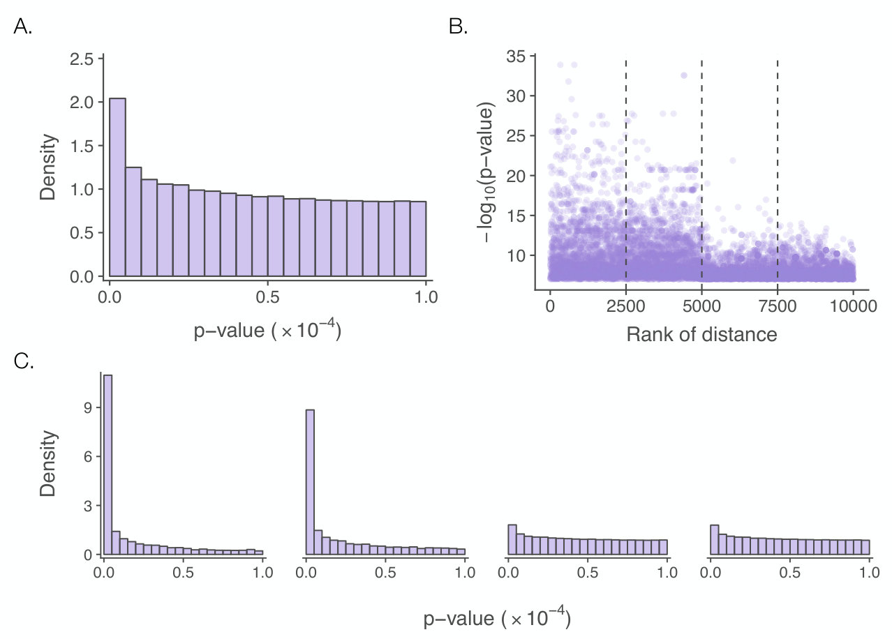 Figure 1
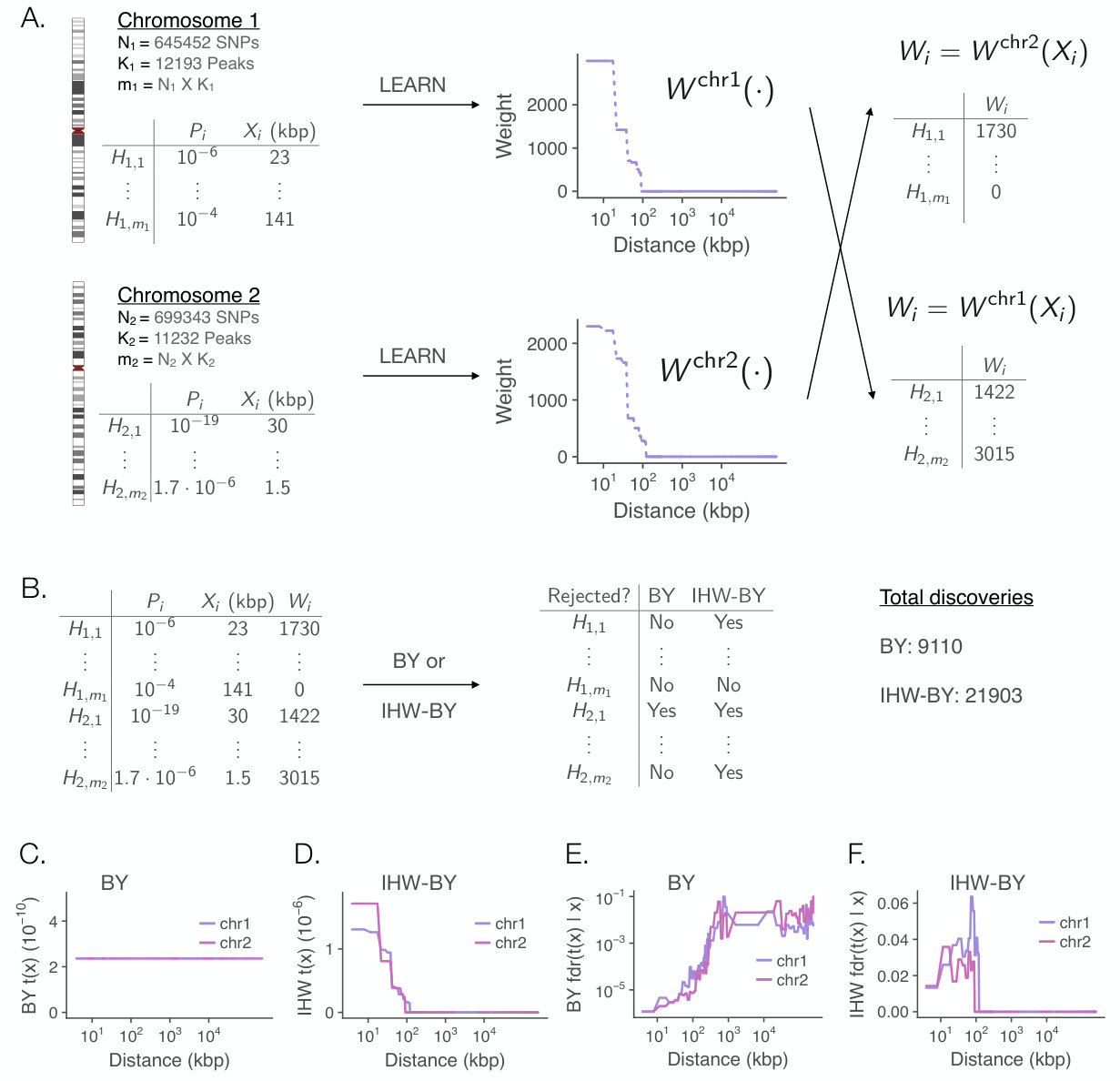 Figure 2
Peer Reviews
No public reviews on file for this paper yet. If you reviewed it on a platform where reviews are public (OpenReview, ICLR, NeurIPS, ICML), you can paste yours below so the community can read it here.
Code & Models
Videos
No videos yet. Explain this paper in a talk, walkthrough, or lecture? Add one.
Covariate powered cross-weighted multiple testing
Nikolaos Ignatiadis1
Wolfgang Huber2
1 Department of Statistics, Stanford University, USA
2 European Molecular Biology Laboratory, Heidelberg, Germany
Summary
A fundamental task in the analysis of datasets with many variables is screening for associations. This can be cast as a multiple testing task, where the objective is achieving high detection power while controlling type I error. We consider hypothesis tests represented by pairs of p-values and covariates , such that if is null. Here, we show how to use information potentially available in the covariates about heterogeneities among hypotheses to increase power compared to conventional procedures that only use the . To this end, we upgrade existing weighted multiple testing procedures through the Independent Hypothesis Weighting (IHW) framework to use data-driven weights that are calculated as a function of the covariates. Finite sample guarantees, e.g., false discovery rate (FDR) control, are derived from cross-weighting, a data-splitting approach that enables learning the weight-covariate function without overfitting as long as the hypotheses can be partitioned into independent folds, with arbitrary within-fold dependence. IHW has increased power compared to methods that do not use covariate information. A key implication of IHW is that hypothesis rejection in common multiple testing setups should not proceed according to the ranking of the p-values, but by an alternative ranking implied by the covariate-weighted p-values.
Keywords: Benjamini-Hochberg, Empirical Bayes, False Discovery Rate, Independent Hypothesis Weighting, Multiple Testing, p-value weighting
1 Introduction
Screening large datasets for interesting associations is a basic operation in statistical data analysis. A frequently taken approach is to enumerate all potential associations, set up a hypothesis test for each of them, summarize the results by the p-values , and select as discoveries all hypotheses with a small enough p-value; typically, this is a small fraction of all hypotheses. More formally, for some cutoff :
[TABLE]
The choice of the cutoff may be data-driven and is determined by a multiple testing procedure, such as those proposed by Bonferroni (1935) or Benjamini and Hochberg (1995), which compute a that provides a defined level of protection against spurious discoveries. Common objectives are control of the family-wise error rate (FWER) or the false discovery rate ().
These procedures operate solely on the list of p-values. Here, we consider situations in which beyond the p-value , side information represented by a covariate is available for each hypothesis. Such side-information reflects heterogeneity among the tests and may —more or less directly—carry information about their different power, or the different prior probabilities of their null hypothesis being true. Suitable covariates are often apparent to domain scientists or to statisticians. We will see that procedures that take into account such side information often have higher power, in the sense that they make more discoveries at the same level of type-I error.
To illustrate, we use a high-throughput genetics dataset by Grubert et al. (2015), who aimed to discover associations between genetic polymorphisms (SNPs) in the human genome and the activity of genomic regions (H3K27ac peaks). The main idea of the analysis of these data, which is presented in more detail in Section 6, is to carry out a hypothesis test for each pair of SNP and region on the same chromosome. On Chromosomes 1 and 2, and SNPs were recorded, and H3K27ac levels were measured in and regions, which amounts to nearly 16 billion () tests. Figure 1 illustrates how the p-value distributions differ as a function of the genomic distance between SNP and region. These differences are consistent with biological domain knowledge: associations across shorter distances are a-priori more plausible and empirically more frequent. Methods that are able to take into account this heterogeneity among the tests should be able to discover more associations at the same , compared to (1), which ignores such side information.
1.1 Independent Hypothesis Weighting
In this paper, we present Independent Hypothesis Weighting (IHW), a flexible framework that can leverage hypothesis heterogeneity to improve power, while retaining finite-sample type-I error control. To explain the method, consider testing hypotheses based on p-values in the situation where we also have access to covariates such that each is independent of the p-value if is a null hypothesis; the codomain of the can be any space (the same for all ). We propose to use a decision rule of the following form in place of (1):
[TABLE]
and is a partition of the hypotheses into disjoint folds, such that the pairs are independent across folds.
There are two salient features to this rule: first, the decision boundary of hypothesis does not only depend on its p-value and the overall cutoff , but also on the weight function of the covariate , where is the codomain of the , and there is one such function for each fold . Second, the notation is used to denote that each of these functions is learned from the data with the proviso that only p-values from the folds excluding are used. We call this proviso cross-weighting.
Conceptually, cross-weighting is related to cross-fitting (Schick, 1986), a method that has been successful in the fields of causal inference (Nie and Wager, 2020; Chernozhukov et al., 2017) and empirical Bayes (Ignatiadis and Wager, 2019) for estimation with high-dimensional nuisance parameters. Analogous to findings in the cross-fitting literature, we will show that naively using plug-in estimators to obtain the weight function tends to overfit, but cross-weighting salvages this at essentially no cost.
1.2 Related work
Previous work has shed light on optimal discovery thresholds in heterogeneous multiple testing. Similar to (2), these thresholds may take the form parametrized in terms of weights that are optimal for controlling the family-wise error rate (FWER) (Roeder and Wasserman, 2009; Peña et al., 2011; Dobriban et al., 2015) or the false discovery rate () (Roquain and Van De Wiel, 2009; Durand, 2019). Furthermore, in the case of control, optimal decision thresholds are known to take the form of contours of equal local false discovery rate (Cai and Sun, 2009; Cai et al., 2019; Efron, 2010; Ferkingstad et al., 2008; Ochoa et al., 2015; Ploner et al., 2006; Scott et al., 2015). Nevertheless, all of these optimal procedures are not implementable, as they depend on unknown properties of the data-generating mechanism. Instead, it has been proposed to apply a plug-in principle: the thresholds are estimated from the data at hand.
Such plug-in approaches however have no guarantees of type-I error control or only do so in an asymptotic limit, as the number of tested hypotheses goes to infinity (Cai and Sun, 2009; Cai et al., 2019; Durand, 2019; Ignatiadis et al., 2016). More importantly, with finite samples, these plug-in methods often exceed the claimed type-I error; we will demonstrate this in Sections 2.1 and 5. This has motivated the provision of case-by-case, ad-hoc modifications, which however still do not provide finite-sample guarantees. For example, Durand (2017) recommends conducting a global test first and only proceeding with multiple testing if the global null hypothesis can be rejected. Cai, Sun, and Wang (2019) use a conservative modification of the density estimator employed by their (asymptotically valid) plug-in approach and show that this controls in simulations with sparse signals. Furthermore, they suggest using the global screen of Durand (2017) first. Ignatiadis, Klaus, Zaugg, and Huber (2016) use cross-weighting (described above) as a heuristic to maintain control in finite samples.
Dispensing with heuristics, several authors have recently provided procedures that are formally justified under full independence of the hypotheses: Li and Barber (2019) propose SABHA, a data-driven, weighted procedure for control which directly confronts potential overfitting. The authors prove finite sample control at an elevated level compared to the nominal ; i.e., at for some . However, their guarantee only applies for their specific weighting scheme, which furthermore is suboptimal even under knowledge of the data-generating process (Lei and Fithian, 2018). Zhang, Xia, Zou, and Tse (2017) and Zhang, Xia, and Zou (2019) use a variant of hypothesis splitting to guarantee high-probability bounds on the false discovery proportion, however their proposals require a minimum number of rejections; otherwise an empty list of discoveries is declared. Closer to our approach is AdaPT (Lei and Fithian, 2018), which uses covariate information to learn covariate-modulated decision boundaries and provides finite sample guarantees. Its construction is based on a variant of the optimal stopping theorem developed by Barber and Candès (2015), which provides the analyst with considerable flexibility in learning these boundaries from the data, while masking information that could lead to overfitting. However, AdaPT has no theoretical guarantees outside of full p-value independence, is tied to control and suffers from a large variance of the false discovery proportion (Korthauer et al., 2019).
Here we propose a general and flexible framework that goes beyond these previous approaches. We formalize hypothesis weighting with weights as a function of covariates and demonstrate that such weights can be learned from the data without overfitting (i.e., losing type-I error control) if we use cross-weighting as in (2). Hence we build upon the hypothesis-splitting idea of Ignatiadis et al. (2016) and demonstrate that it can be used not merely as a heuristic, but instead as a theoretically grounded and principled way of conducting multiple testing with side-information that has far reaching applications. The Independent Hypothesis Weighting method provides finite sample guarantees for multiple type-I measures, such as the , the FWER and the -FWER, unlike previous proposals that are tied to the . IHW provides a clean way to deal with dependent settings, as it allows arbitrary dependence within folds. Finally, IHW provides the researcher with flexibility in choosing any weighting scheme that would be appropriate for the data at hand, but we also recommend a default scheme and provide a software implementation in the form of an R package.
1.3 Outline
In Section 2, we provide an overview of weighted multiple testing and explain our proposal in the context of control under full independence of hypothesis tests. Section 3 extends the results to dependence, and to control of the -FWER. Section 4 describes a framework for learning weighting rules. Section 5 provides simulation results, and Section 6 presents the high-throughput biology example from Figure 1. Section 7 discusses further relationships to previous work, and Section 8 concludes with a discussion.
2 Weighted and cross-weighted multiple testing
A multiple testing procedure operates on data for hypotheses and declares hypotheses as rejections (“discoveries”). Among these, will be nulls, i.e., the procedure will commit type I errors. The goal is to make as many discoveries as possible while retaining (stochastic) guarantees that is acceptable. Concretely, one possible objective is to control the family-wise error rate, defined as FWER , or the -FWER . In exploratory situations, a typically less stringent objective is to control the false discovery rate (), i.e., the expectation of the false discovery proportion (FDP), namely (Benjamini and Hochberg, 1995).
Typically the data for each hypothesis are summarized into a single number, the p-value , and a rule of form (1) is applied. However, in the presence of heterogeneity across tests, it might be suboptimal to use such a decision rule that treats all hypotheses exchangeably. Weighted multiple testing (Genovese, Roeder, and Wasserman, 2006) is a flexible way of encoding prior information and differentially prioritizing the hypotheses. Multiple testing weights are defined as non-negative numbers such that . Then, a weighted multiple testing decision rule takes the following form:
[TABLE]
Here is a fixed number, of which more below, and as in (1), the cutoff may be data-driven. A larger implies that it is easier to reject hypothesis . We first review two procedures for choosing .
Definition 1** (Weighted -Bonferroni).**
The -FWER can be controlled at level by applying the weighted -Bonferroni procedure (Romano and Wolf, 2010), which takes the form (3) with deterministic cutoff and . The case is the weighted Bonferroni procedure proposed by Genovese et al. (2006).
Definition 2** (-censored, weighted Benjamini-Hochberg).**
The can be controlled at level by applying the -censored, weighted Benjamini-Hochberg procedure, which takes the form (3) with fixed and data-driven cutoff specified as:
[TABLE]
The weighted Benjamini-Hochberg (BH) procedure of Genovese, Roeder, and Wasserman (2006) is the special case . The more general form was proposed by Li and Barber (2019) and will be employed for our theoretical guarantees in the following. The number of rejections of -censored BH is non-decreasing in , so that a procedure with smaller will never make more discoveries. However, for large , say , the discovery set will be equal to that with , as long as weighted BH with did not reject a p-value .
In decision rule (3), the weights are denoted by lower-case letters. This reflects the fact that existing results treat these weights as deterministic—as prior knowledge that a researcher has to specify before seeing the p-values (Genovese, Roeder, and Wasserman, 2006; Blanchard and Roquain, 2008; Habiger, 2017; Roquain and Van De Wiel, 2009; Ramdas, Barber, Wainwright, and Jordan, 2019). The main goal of this work is to let the weights depend on the data at hand—they are thus denoted as random variables —while providing finite-sample guarantees. Such data-dependent weighting has been recognized as an important open problem (Benjamini, 2008; Roquain and Van De Wiel, 2009) that is essential for dealing with large scale multiple testing. To the best of our knowledge, no solution has been provided so far. Existing proposals for data-driven weighting either explicitly account for overfitting by establishing control at an elevated level compared to nominal (Li and Barber, 2019) or only provide guarantees in the asymptotic limit (Hu, Zhao, and Zhou, 2010; Ignatiadis, Klaus, Zaugg, and Huber, 2016; Durand, 2019; Zhao and Zhang, 2014; Wang, 2018; Roeder, Devlin, and Wasserman, 2007).
2.1 Example: Group Benjamini-Hochberg with cross-weighting
We first provide a rudimentary version of our method that is applicable to situations with categorical (or suitably categorized) covariates . This setting is called multiple testing with groups; each group consists of hypotheses whose covariate takes on the same value. Our method builds upon the Group Benjamini-Hochberg (GBH) method proposed by Hu et al. (2010) to improve power compared to BH by using the group structure. GBH consists of first estimating the proportion of null hypotheses in each group by , weighting each hypothesis proportionally to and finally applying the weighted BH procedure. Algorithm 1 describes the method in detail111A simplification is that in Algorithm 1, the weights are specified so that . In contrast, in the original GBH paper (Hu et al., 2010), the weights are less conservative and satisfy . This inflation ensures that in the oracle case of known , the of GBH is exactly equal to . We return to the issue of null proportion adaptivity in Section 2.3 and Theorem 2; in the case of GBH it may be regained by employing the optional step in Algorithm 1, cf. Ramdas et al. (2019)., using the estimator of Storey et al. (2004) applied to the grouped setting, analogous to Sankaran and Holmes (2014).
Hu, Zhao, and Zhou (2010) provide the following guarantees for GBH: in the oracle situation where the are known, GBH controls the . In the asymptotic limit where the number of groups is fixed, the number of hypotheses in each group grows to infinity and for all , GBH controls the . Furthermore, sufficient conditions are given so that asymptotically GBH is at least as powerful as BH. The asymptotics, however, do not necessarily apply for finite , the number of hypotheses per group, as shown by simulations summarized in Figure 2. Intuitively, the reason is that some groups will randomly be enriched for smaller than expected p-values (and some for larger than expected ones), and the method further up-weights the former set of null p-values.
Our solution is to use cross-weighting. We assign each hypothesis to one of folds – randomly and independently of its p-value and covariate – and then calculate weights out-of-fold, as elaborated in Algorithm 2. With cross-weighting, a null p-value that is small by chance cannot lead to an upweighting of itself. control is restored, as shown in Figure 2. On the other hand, if the weights are determined not just by noise, but by true signal, then IHW-GBH, just as GBH, has increased power compared to BH, as we show in a more comprehensive simulation study in Section 5.1. If furthermore remains fixed as , then GBH and IHW-GBH are asymptotically equivalent (Corollary 2).
2.2 IHW: A family of multiple testing procedures
We now generalize the IHW-GBH procedure beyond categorical covariates, the GBH weighting scheme and the weighted BH procedure (Def. 2): we seek a general way of applying weighted multiple testing methods with data-driven weights when covariates —not necessarily categorical—are available. Our approach consists of two ingredients: first, we only consider weights that are functions of the covariates , i.e., . The second ingredient is cross-weighting: we partition our hypotheses into disjoint folds222Our baseline proposal is to construct the partition by splitting the set into (the default in the IHW software package is ) equally sized folds randomly. Alternatively, domain specific knowledge can be used to derive folds that minimize across-fold dependence, cf. the example in Section 6. . Then, in determining the weight for hypothesis , we set , where the weight function is learned from data outside fold and the weights are normalized, typically such that . This overall framework is summarized in Algorithm 3.
In Sections 2.3 and 3.2 we provide formal guarantees of finite-sample type-I error control for the IHW algorithm, under the condition that the weighted multiple testing procedure is weighted BH with -censoring or weighted -Bonferroni. We will discuss how to learn weight functions for general (non-categorical) covariates in Section 4.
2.3 Finite-sample FDR control with cross-weighting under independence
To derive formal guarantees for Algorithm 3, we set out with a sufficient distributional assumption that contains several independence relationships. In Section 3, we will consider more general dependence structures.
Assumption 1** (Distributional setting under independence).**
Let , be333We use the notation . (p-value, covariate) pairs and be the index set of null hypotheses. We assume that:
- (a1)
The null pairs are jointly independent. 2. (a2)
The null pairs are independent of the alternative pairs . 3. (b )
For , it holds that is independent of . 4. (c )
For , is super-uniform, i.e., for all .
To parse this assumption, let us first consider two important special cases: (i) marginalizing over the , so that we only have access to p-values, and (ii) deterministic . In both cases, Assumption 1 reduces to (a1’) are jointly independent, (a2’) independent of the alternative p-values and (c). Of these, (a1’) and (a2’), while admittedly strong, are a typical starting point for proving finite-sample results for multiple testing procedures, even in the absence of covariates: Liang and Nettleton (2012) call it the null independence assumption. In the setting with covariates, these are also assumptions made by Li and Barber (2019, Theorem 1) and Lei and Fithian (2018, Theorem 1). Cai et al. (2019) also assume full independence of hypotheses. The super-uniformity; also called conservativeness, of the null p-values (c) is also a standard assumption in multiple testing (Blanchard and Roquain, 2008). Li and Barber (2019) make a stronger assumption than (c).
The case of deterministic is important, since for example the genomic distance between SNPs and peaks in our motivating example in Figure 1 is a deterministic covariate. See Supplement S6.1 for additional examples. Nevertheless, we formulate results for the more general case to also handle situations in which the covariate is calculated from the same data that are used to calculate the p-value . For instance, Cai et al. (2019) consider simultaneous two-sample testing, and construct an ancillary that is independent of the -statistic (and thus also the p-value) under the null hypothesis; we revisit their construction in the simulation study of Section 5.3. Assumption 1(b) is crucial in ensuring that knowledge of does not influence the null distribution. Cai et al. (2019) call it a ”principle for information extraction”; cf. Bourgon et al. (2010); Boca and Leek (2018) for further elaborations on this assumption and Supplement S6.2 for more examples of random covariates.
Next, we state two specifications on the weighting mechanism used. Unlike Assumption 1, the applicability of which depends on the generally unknown data-generating mechanism, these are entirely under the control of the analyst.
Specification 1** (Honest weighting).**
Consider a partition of into folds , i.e., and are disjoint, and define . The partition is assigned independently of . Then, the data-driven weights are honest with respect to the partition if:
- (a)
is a function of only and for all and all . 2. (b)
The weights in fold average to , i.e., for all . 3. (c)
for all .
We call this specification “honest weighting”, borrowing terminology from the honest tree construction of Wager and Athey (2018), who call a regression tree honest if the set of observations used to determine its structure is disjoint from the set of observations used for prediction in the leaves. Specification 1 encapsulates our idea of cross-weighting. Informally, it says that the weight of hypothesis should not depend on its p-value . As already shown in Figure 2, without honesty it is easy to overfit the data. Part (b) of the definition encapsulates a fixed weighting budget (Genovese, Roeder, and Wasserman, 2006). Instead of merely requiring , the budget is restricted within each fold, to prevent information leakage across folds through the total magnitude of the weights.
Honesty suffices to guarantee type-I error control in some cases, for example for the weighted -Bonferroni procedure (Section 3.2 and Theorem 3). However, for the -censored, weighted BH procedure with data-driven weights, we require one further condition on the weights, which was proposed by Li and Barber (2019) and states that the magnitude of p-values less than or equal to must be concealed from the weighting algorithm.
Specification 2** (-censored weighting).**
The weights are called -censored for if they depend on the p-values only through .
We are ready to state the first result:
Theorem 1** (IHW-BH controls the under honesty and -censored weighting).**
Let satisfy Assumption 1. Furthermore assume that we construct data-driven weights that are honest (Specification 1) and -censored (Specification 2) for some . Then the -censored, weighted BH procedure (Definition 2) with p-values and weights controls the at the nominal level .
The intuition for this theorem is the following: in the weighted BH algorithm (Definition 2), the rejection threshold of a null p-value depends on its weight and the total number of rejections . Assumption 1 and honest weighting (Specification 1) ensure that a null p-value cannot influence its own weight. However, tests can coordinate adversarially by weighting each other in a way that increases and potentially leads to their own rejection. Supplement S1.3 provides an example of how such adversarial coordination can break -control guarantees, even though honesty holds. However, under -censoring, the only p-values that can coordinate through weight assignment are the ones . These p-values are also excluded from being rejected and so control is restored.
As a corollary, we get the following result:
Corollary 1** (IHW-GBH controls the ).**
Let satisfy Assumption 1, then the IHW-GBH procedure (without the null proportion adaptivity step) described in Algorithm 2 controls the at the nominal level .
Proof.
By construction, the weights of IHW-GBH are honest and -censored. ∎
A shortcoming of IHW-BH with weights that satisfy is that FDR is controlled at , where and IHW-BH can thus be needlessly conservative. Motivated by null-proportion adaptive methods for unweighted BH (Storey, Taylor, and Siegmund, 2004) and weighted BH with deterministic weights (Habiger, 2017; Ramdas, Barber, Wainwright, and Jordan, 2019), we estimate within fold by
[TABLE]
and use these estimates to inflate the weights . We have the following result:
Theorem 2** (IHW-Storey controls the under honesty and -censored weighting).**
Assume that all assumptions of Theorem 1 are satisfied. Next let be defined as in (5) and define null-proportion adaptive weights as for . Then the -censored, weighted BH procedure (Definition 2) with p-values and weights controls the at the nominal level .
A direct application of this theorem is that the statement of Corollary 1 also holds for the null-proportion adaptive version of IHW-GBH (cf. Algorithm 2). This provides power gains in situations where the null proportion is substantially smaller than 1 at least in some regions of the covariate space, since then it will be the case that , thus increasing the total weight budget.
2.4 FDR asymptotics with cross-weighting under independence
While the primary focus of this paper is on finite-sample guarantees and performance in simulations, in this section we provide asymptotic results for that serve three purposes: first, they demonstrate how cross-weighting enables a streamlined proof of asymptotic control under standard assumptions on while dispensing of requirements on the class of weight functions. Second, they show that in situations in which there is sufficient signal and the data-driven weight function has approached its asymptotic limit, no power is lost by using cross-weighting. Third, they show that in an asymptotic regime, IHW-BH controls the without a need for -censoring (Specification 2). On the other hand, our aim here is not to provide the sharpest asymptotics under the weakest conditions, but just to provide these conceptual insights.
We develop the asymptotics using the following Bayesian model (Ferkingstad et al., 2008; Lei and Fithian, 2018; Deb et al., 2021), which we call the conditional two-groups model and which extends the two-groups model of Storey (2003) and Efron, Tibshirani, Storey, and Tusher (2001):
[TABLE]
We also define : the distribution of given . The distribution can vary from test to test because of varying null probabilities and/or alternative distributions , depending on the value of its covariate .
Since is a changing parameter in the asymptotics, it is useful to formalize what “learning a weight function” entails and use more involved notation:
Specification 3** (Weighting scheme).**
A weighting scheme is a mechanism that, for any finite subset , uses samples to learn a weight function . We assume that the learned weight function does not excessively upweight individual hypotheses, i.e., there exists such that
[TABLE]
Given independent draws from (6) and a weighting scheme (Specification 7), we seek to apply learned weights in conjunction with weighted BH (Definition 2). We consider two possibilities:
Naive weighted BH: We use all data to learn and let for , such that the weights average to (i.e., ). Then we apply the weighted BH procedure with p-values and weights . 2. 2.
IHW-BH: We partition into disjoint folds , independently of . Then we apply Algorithm 3 in conjunction with weighted BH, i.e., for each fold , we apply the weighting scheme on and for set weight and such that the weights average to in that fold (i.e., ). Then we apply weighted BH with p-values and weights . We note that the data-driven weights are honest (Specification 1) by construction. However, for the asymptotics, we do not require -censoring (Specification 2), but instead require the mild technical condition (7).
Proposition 1**.**
Let be i.i.d. from the conditional two-groups model (6) satisfying regularity Assumption 3 (in Supplement S2). If the partition satisfies as for all , then555See Supplement S2 for the proof and formal statements.:
- (a)
There exists a weighting scheme satisfying Specification 7, such that the naive weighted BH procedure asymptotically does not control the . 2. (b)
For any weighting scheme satisfying Specification 7, the IHW-BH procedure asymptotically controls the . 3. (c)
Consider a weighting scheme that converges in probability to a deterministic limiting weight function ,
[TABLE]
Then, the naive weighted BH and IHW-BH procedures have the same power asymptotically.
Proof idea for (a) and (b):.
The proof of Storey et al. (2004) for asymptotic control of BH argues that by the Glivenko-Cantelli theorem, and similarly for the subset of null hypotheses. A consequence is that the BH estimator of the false discovery rate is asymptotically uniformly conservative over all thresholds , which in turn implies asymptotic control. Extending this argument to the weighted case requires uniform convergence: .
For data-driven weights, this can be achieved by learning the weight function from a suitably restricted class . Du and Zhang (2014); Ignatiadis et al. (2016); Durand (2019) all use such that the functions are -Glivenko-Cantelli (van der Vaart, 2000). Similarly, Li and Barber (2019) consider with low Rademacher complexity. On the other hand, if convergence is not uniform (e.g., if we are free to choose any weights satisfying Specification 7), then we can find regions of -space that are enriched for small p-values merely by chance, upweight them, and violate control (cf. Figure 2).
Instead, through cross-weighting, the richness of is irrelevant: upon conditioning on other folds, in fold are i.i.d., and thus the one-dimensional Glivenko-Cantelli result applies. ∎
In words, while data-driven weights can lead to overfitting (a), cross-weighting universally alleviates this (b). A further upshot of (b) is that it dispenses with the requirement for -censored weights (Specification 2). Finally, the objection may be raised to cross-weighting that it drops data and should thus be less powerful than a procedure that uses all the data. However, (c) shows that asymptotically one loses no power by using cross-weighting if the weighting procedure is well-behaved, i.e., the weights asymptotically converge to a limit.
As a corollary of Proposition 1, we have that:
Corollary 2** (IHW-GBH asymptotics).**
Under the assumptions of Proposition 1 with for fixed , the GBH and IHW-GBH procedures without null proportion adaptivity, described in Algorithms 1 and 2, have the same power asymptotically.
Proof.
In Supplement S2.4, we verify (7) and the condition from part (c) of Proposition 1. ∎
At this point, we note that Durand (2019), motivated by a preprint version of this work, derived the following related and elegant result: in the setting with a finite discrete space, Durand (2019, Theorem 7.1.) constructs a cross-weighted procedure that asymptotically controls the and simultaneously achieves the power of the optimal weighted procedure.
3 Extension to dependence
3.1 The key assumption: Independence across folds, dependence within
Assumption 1 made the strong assumption of joint independence of all null p-values and was sufficient for the results presented in Section 2. Real data commonly deviate from this assumption. The consequences of such deviations on the applicability of results derived using independence assumptions are typically difficult to reason about. It is therefore desirable to construct guarantees that can be derived from weaker assumptions that are closer to realistic patterns of dependence.
Assumption 2** (Distributional setting with dependence).**
Let , be (p-value, covariate) pairs, be folds of a partition of that is defined based on information independent of , and let the index set of null hypotheses. We assume that:
- (a)
The (p-value, covariate) pairs are independent across folds , but may be dependent within each fold. Formally, are jointly independent. 2. (b)
For , it holds that is independent of . 3. (c)
For , is super-uniform, i.e., for all .
Let us compare Assumption 2 to Assumption 1. Parts 2(b, c) are mild. Part 2(c) is identical to 1(c) and standard in multiple testing. Part 2(b) is analogous to 1(b), albeit stronger, since we are conditioning on the full vector of . Nevertheless, 2(b) is implied by 1(a,b). In the important case where the are deterministic, 1(b) trivially holds. But it also allows for situations where, for instance, the are random spatial locations. In this case, we may expect p-values with similar to be correlated. Assumption 2(b) then means that knowing the locations of all hypotheses provides no information about a single null p-value .
The critical assumption is 2(a). Without covariates, the assumption implies that is a partition of p-values into independent blocks. This is not an assumption typically encountered in the multiple testing literature, although it has appeared e.g., in Heesen and Janssen (2015); Guo and Sarkar (2019). It is fundamental to the cross-weighting approach, the core idea of which is to avoid any dependence between each individual null p-value and its data-driven weight . Cross-weighting ensures that is determined based on and p-values from the other folds, but not . This would no longer be true with dependence across folds. This observation is analogous to a similar phenomenon in cross-validation. In Chapter 7.1 of the Elements of Statistical Learning, Hastie, Tibshirani, and Friedman (2009) caution practitioners to split data into independent folds when evaluating a supervised learning method by cross-validation (CV): if the folds are not independent, the CV estimates of prediction error are not reliable.
From the application perspective, the assumption is practical: domain experts often have sufficient understanding of their data to find suitable partitions of the hypotheses into independent blocks. In the example from Figure 1, further detailed in Section 6, it is plausible to assume that the data for hypotheses located on different chromosomes are independent, or at least that any potential dependences are negligible. As another example, for covariates that correspond to spatial or temporal positions, hypotheses that are sufficiently far away from each other will be independent if the dependences are mediated by spatial or temporal proximity.
We note that all other existing methods for multiple testing with covariates that provide control assume either full independence (Lei and Fithian, 2018; Cai et al., 2019), weak dependence (Li and Barber, 2019) or the ability to consistently estimate the joint distribution of all hypotheses (Sun and Cai, 2009). Thus, Assumption 2 is a practical starting point towards dealing with common patterns of dependence encountered in real data.
Next, we describe two multiple testing methods with data-driven weights that have provable type-I error guarantees under dependence.
3.2 -FWER control with cross-weighting under dependence
-FWER control is achieved by applying cross-weighting in conjunction with the weighted -Bonferroni procedure of Definition 1. We are not aware of existing procedures with data-driven weights and finite-sample -FWER control. Existing proposals provide asymptotic guarantees (Wang, 2018).
The proof is direct and without technical complications. We provide it here in the main text, since it shows the key idea behind cross-weighting: each null p-value is independent of its weight , and this protects against overfitting.
Theorem 3**.**
Let satisfy Assumption 2 (or Assumption 1) with respect to the partition . Furthermore assume that we construct data-driven weights that are honest w.r.t. (Specification 1). Then the weighted -Bonferroni procedure (Definition 1) with p-values and weights controls the at the nominal level .
Proof.
We first show that is independent of () for any . Without loss of generality, . By honesty, is a function only of the p-values in the other folds, and all covariates . It thus suffices to argue that is independent of . This follows from Assumption 2 (resp. Assumption 1). We next bound the .
[TABLE]
Note that in , we used the fact that for it holds that is super-uniform and is independent of . In the last step we used that honesty ensures that . ∎
3.3 FDR control with cross-weighting under dependence
We recall the basic procedure for controlling with (deterministic) weights under arbitrary dependence:
Definition 3** (Weighted Benjamini-Yekutieli (wBY) (Benjamini and Yekutieli, 2001; Blanchard and Roquain, 2008)).**
Consider p-values with arbitrary dependence such that the null p-values are super-uniform. Furthermore consider deterministic weights such that . Then the is controlled at level by applying the weighted Benjamini-Yekutieli procedure at level , i.e., the weighted Benjamini-Hochberg procedure (Definition 2) with at level .
We now show that applying the weighted BY procedure with cross-weighting controls the under Assumption 2.
Theorem 4** (IHW-BY controls the under honesty and independent folds).**
Let satisfy Assumption 2 with respect to the partition . Furthermore assume that we construct data-driven weights that are honest w.r.t. (Specification 1). Then the weighted BY procedure (Definition 3) with p-values and weights controls the at the nominal level .
To demonstrate that honesty is essential for the result of Theorem 4, we next describe two plausible candidate methods for FDR control with covariates that do not control :
Example 1** (BY with arbitrary data-driven weights does not control under Assumption 2).**
Theorem 4 may appear as a consequence of Theorem 4.2. of Blanchard and Roquain (2008), who extended the results of Benjamini and Yekutieli (2001) and proved that the weighted BY procedure (Definition 3) controls the for any choice of weights and any p-value distribution. However, their result holds only for deterministic weights and not for data-driven weights, as we now demonstrate.
Proof.
We generate satisfying Assumption 2 and under the global null as follows: fix for . We consider deterministic covariates and the partition . We first draw a permutation from the uniform measure on the permutation group of . Next we independently draw: for and let . Finally we draw independent . Weights are chosen as follows: Let and then let . Then the of weighted BY at is equal to as long as , as we now show:
Since the smallest p-value in is uniformly distributed on , it follows that with probability , and hence . gets rejected and so almost surely. ∎
In contrast, control would be guaranteed, had we used weights derived through cross-weighting. BY with -censored weights (Specification 2) also does not control , cf. Supplement S1.6.
Example 2** (AdaPT with BY correction does not control under Assumption 2).**
Lei and Fithian (2018) prove control for AdaPT under full independence (cf. Assumption 1). Here we demonstrate that even with the Benjamini-Yekutieli correction, i.e., at level and -censoring (Specification 2), AdaPT does not control under Assumption 2.
Proof.
We generate satisfying Assumption 2 and under the global null as follows: we fix and consider the partition . We take constant covariates for all and draw . Finally we set and . We then run the AdaPT algorithm at level with the initialization specified in Lei and Fithian (2018). Then as long as , as we now show:
As specified in Section 4.4.1 of Lei and Fithian (2018), the AdaPT algorithm is initialized at threshold . Now call the event that . On the event , on the first step of the algorithm, AdaPT estimates the FDP (cf. (14)) as , which is equal to if and equal to otherwise. In both cases, the estimated FDP is less or equal than and thus less than under our assumption on . Thus AdaPT immediately terminates, rejecting all p-values in , and so . Similarly on the event and . Finally, note that the above procedure is -censored with . ∎
4 Learning powerful weighting rules
Sections 2 and 3 focused on sufficient conditions for type-I error control, but did not address power. These conditions leave considerable flexibility in the choice of the class of possible weight functions, and in the method of selecting (or “learning”) these functions, given the data. This flexibility gives the analyst the opportunity to use domain-specific as well as statistical knowledge to make choices that have desirable type-II error properties. Nevertheless, it is useful to provide a default algorithm that works well across a range of settings. To this end, here we describe two schemes for learning weight functions, one for weighted -Bonferroni and one for weighted BH. Both rely on positing the approximate applicability of model (6), estimating quantities appearing therein and solving a convex program to find a weight function that optimizes the expected number of discoveries.
4.1 Learning weights for IHW -Bonferroni
The weighted -Bonferroni procedure with weight function rejects hypotheses that satisfy . Under Model (6), a weight function maximizing the expected number of discoveries is one that maximizes . To derive honest weights (Specification 1) that approximately maximize this objective, we learn for each fold separately as follows: first we estimate from Model (6) by using only p-values and covariates outside of fold . Next, identifying with the function’s values evaluated at the , i.e. we solve the -dimensional problem with optimization variables :
[TABLE]
This setting allows for conditional distributions that are different for tests with different covariates . We consider estimators that are concave in for all . This has the advantage of turning (8) into a convex optimization program, which is often tractable. Concavity of the distribution of p-values is a reasonable assumption and often provides a good fit to multiple testing datasets (Strimmer, 2008b; Genovese, Roeder, and Wasserman, 2006). However, the procedure works even when the concavity assumption does not hold: given any (potentially non-concave) pilot estimator of the conditional distribution function , we can project it onto the set of concave distribution functions and solve the optimization problem with the projected distribution functions. We interpret the resulting procedure as a convex relaxation of (8) that makes computation tractable.
With this setup, we are ready to state a concrete weighting scheme, which proceeds in three steps: first, discretize the into a finite number of bins defined, e.g., by quantile slicing or as the leaves of a tree. Second, estimate by the Grenander estimator (Grenander, 1956), i.e., the least concave majorant of the empirical cumulative distribution function of the p-values with and . Third, solve (8) for each by linear programming. The reason that (8) may be expressed as a linear program is that the Grenander estimator is always concave in and piecewise linear. We provide the details of the estimation and optimization procedures in Supplement S4.1; the computational complexity scales as .
An alternative ansatz is to specify and in the conditional two-groups model (6) parametrically. For instance, we may consider for
[TABLE]
Such a Beta-Uniform mixture model has been considered in the setting without covariates, e.g., by Allison et al. (2002); Klaus and Strimmer (2011) and with covariates by Lei and Fithian (2018). In Supplement S4.2 we explain how to learn the parameters of the model using the expectation-maximization algorithm and how to optimize (8).
4.2 Learning weights for IHW Benjamini-Hochberg
Our starting point for deriving powerful weight functions for the weighted BH procedure (Definition 2) is again the conditional two-groups model (6). We seek a threshold function , such that the multiple testing procedure that rejects hypotheses with satisfies the following two properties: first, the marginal , defined as is bounded by , i.e., and second, the expected number of discoveries is large666Such a Bayesian, Neyman-Pearson type procedure is motivated by the asymptotic equivalence between the frequentist and the mFDR (Genovese and Wasserman, 2004; Sun and Cai, 2007; Cai and Sun, 2009; Cai et al., 2019).. Similarly to our Bonferroni construction, we learn the threshold function for each fold separately. To this end, we estimate and out of fold. Noting that is implied by , we propose solving:
[TABLE]
As our goal is to apply the weighted BH procedure, we convert these thresholds into weights through normalization: for , set , unless the denominator is [math], in which case . A few remarks are in order: similarly to optimization problem (8), (10) is also a convex program if is concave in for all , and may be expressed as a linear program if the Grenander estimator is used. We thus again suggest to discretize and estimate distributions with the Grenander estimator. If the weights will be applied in conjunction with the weighted BH algorithm, we suggest to simply set . This optimization and estimation scheme was proposed by Ignatiadis et al. (2016). Alternatively, may be estimated by applying Storey’s null proportion estimator (Storey et al., 2004) to all hypotheses outside fold that fall into the same bin as . Details of the estimation and optimization procedures are provided in Supplement S4.1.
The weights constructed above are honest (Specification 1). Yet, in view of Theorems 1 and 2, it might appear unsatisfying that do not satisfy the -censored weights condition (Specification 2). In our experience, the proposed procedure with the Grenander estimator does not overfit and controls the . This is corroborated by extensive simulations below and by the asymptotic guarantees of Proposition 1.
Our alternative proposal, which satisfies -censoring (Specification 2), is to fit the Beta-Uniform mixture model (LABEL:eq:betamix_simulation_model). The EM algorithm may be modified to accommodate for censored knowledge of ; cf. Markitsis and Lai (2010) in the setting without covariates. Furthermore, under model (LABEL:eq:betamix_simulation_model), the solution to problem (10) lies on a contour of equal conditional local fdr (cf. Theorem 2 in Lei and Fithian (2018)), and this fact facilitates the optimization. We describe the steps in more detail in Supplement S4.2.
Finally, we use the same framework to derive weights for the weighted Benjamini-Yekutieli procedure (Definition 3): we proceed as for weighted BH but solve (10) with replaced by . In this case, honesty suffices for control (Theorem 4).
5 Numerical experiments
Our goal in this section is to corroborate through simulations of three important settings—grouped multiple testing, multiple testing with continuous covariates and simultaneous two-sample tests—the following claims: first, some methods with asymptotic FDR control guarantees do not control FDR in finite samples. Second, IHW is a flexible framework for multiple testing, its main advantage over other methods being finite sample error control (due to cross-weighting), while remaining competitive in terms of power. Throughout this section, we define power as
[TABLE]
The expectation, just as the , is evaluated through averaging over Monte Carlo replicates.
5.1 Grouped multiple testing
We first consider the multiple testing problem with groups, i.e, with categorical covariates . In each simulation we generate , independently, as follows
[TABLE]
In words, there are 40 latent groups defined by , each with 500 hypotheses. A quarter of the groups has non-nulls, three quarters do not. The alternative signal strength and null proportion vary linearly across non-null groups. Parameters are chosen so that the overall proportion of nulls is . We then coarsen to , with varying across simulations; is non-latent, i.e., visible to the algorithm. For example, for , takes on only two levels (2 groups), while for , takes on all 40 levels. We also use the above configuration of covariates and simulate under the global null by drawing all p-values from the uniform distribution.
We compare the following seven methods:
The Benjamini-Hochberg (BH) method (Benjamini and Hochberg, 1995), which ignores the covariates . 2. 2.
The stratified BH procedure (SBH) (Sun et al., 2006; Efron, 2008), wherein the BH procedure is applied times separately to p-values corresponding to different levels of . 3. 3.
The Clfdr (conditional local fdr) procedure of Cai and Sun (2009), which applies an optimal decision rule that rejects hypotheses with a low value of the group-wise local fdr (cf. Algorithm 4 in Supplement S3). We apply a data-driven version of the oracle rule by estimating local fdrs within each group with the fdrtool CRAN Package (Strimmer, 2008a), which estimates marginal densities with the Grenander estimator. 4. 4.
The Group Benjamini-Hochberg (GBH) procedure of Hu et al. (2010) with null-proportion adaptivity, as described in Algorithm 1 (). 5. 5.
The IHW-GBH procedure with null-proportion adaptivity, as described in Algorithm 2 () with hypotheses randomly split into 5 folds. 6. 6.
The IHW-Storey-Grenander procedure: the IHW-Storey method (Theorem 2) with hypotheses randomly split into 5 folds and data-driven weights based on the Grenander estimator described in Section 4.2 and Supplement S4.1. 7. 7.
The Structure Adaptive Benjamini-Hochberg algorithm (SABHA) by Li and Barber (2019): SABHA first estimates for each group by solving a joint convex optimization problem. Then, the -censored, weighted BH procedure is applied with weights . We set the tuning parameters of group-wise SABHA to following Section 7.1 of Li and Barber (2019).
All of the above methods provably control asymptotically, as , the number of groups remains fixed and there is signal in the data, but only BH and IHW-GBH have provable finite-sample control at and SABHA at (Li and Barber, 2019, Lemma 2).
Results are shown in Figure 3. Under the global null (Fig. 3A), SBH strongly overfits, since under the global null the is equivalent to the FWER, so it would need to pay a Bonferroni correction to apply BH separately to each group. Clfdr has much below nominal for a small number of groups (the oracle local fdr procedure would not reject anything under the global null), but as the number of groups increases, it no longer controls . We further discuss this below. All other methods control in this setting. For GBH, however, recall Fig. 2 for a situation where it does display a pronounced loss of control.
For the simulations with signal (Fig. 3B, C) we make the following observations: as increases, the covariates become more informative, hence in principle power can be increased. Indeed this is precisely what we observe (Fig. 3C) for the grouped methods that do not directly estimate the distribution in each group (all methods except Clfdr and IHW-Storey-Grenander). The power of BH remains constant. After BH, the least powerful procedure appears to be SABHA; the suboptimality of its weighting scheme has been previously pointed out (Lei and Fithian, 2018). We also observe that IHW-GBH matches the power of GBH and has the added advantage of provable finite-sample control. Regarding the methods that estimate the distribution, when is small relative to , then the Grenander estimator can precisely estimate the distribution in each bin. This translates into the Clfdr procedure and IHW-Storey-Grenander outperforming the other methods at small ; indeed Clfdr is provably asymptotically the most powerful procedure in this setting. However, as increases and the amount of data in each group decreases, the distributions are not estimated as accurately. The consequence for Clfdr is loss of control, while IHW-Storey-Grenander retains control due to cross-weighting. In conclusion, in this set of simulations, IHW is the most powerful method of those that control .
5.2 Multiple testing with continuous covariates
In this section we explore a setting with a two-dimensional, continuous covariate . We seek to compare IHW, AdaPT and local fdr based methods with an emphasis on understanding behavior under model-misspecification (to be made precise momentarily). We simulate independent from the conditional two-groups model (6) with the following choices for and :
[TABLE]
is a parameter that varies across simulation settings. The two-dimensional covariates modulate both the null proportion and the signal in the alternative density. We compare six methods.
The Benjamini-Hochberg (BH) (Benjamini and Hochberg, 1995) method ignoring . 2. 2.
The oracle Clfdr procedure (Clfdr-oracle) that rejects hypotheses with a small conditional local , with a threshold chosen through Algorithm 4 in Supplement S3. This procedure achieves an optimal trade-off between the false nondiscovery rate and the false discovery rate, cf. Sun and Cai (2007); Cai and Sun (2009). Clfdr-oracle, however, would not be available to an analyst, as it assumes oracle knowledge of the components (LABEL:eq:adapt_simulation_model) in model (6). 3. 3.
The IHW-BH-Grenander procedure, similarly to the previous section, but without null-proportion adaptivity (i.e., with IHW-BH instead of IHW-Storey). The covariates are binned into equal volume bins.
Furthermore, we compare three methods that fit Model (LABEL:eq:betamix_simulation_model) as a misspecified working model for the true model (LABEL:eq:adapt_simulation_model) using the EM algorithm (details in Supplement S4.2).
Clfdr-EM: this is the same as Clfdr-oracle, but instead of true quantities we use the ones estimated by maximum likelihood on the misspecified model (LABEL:eq:betamix_simulation_model). We employ the EM algorithm since the status is unknown. 2. 5.
IHW-Storey-BetaMix: this is the IHW-Storey method with hypotheses split randomly into 5 folds and weights derived from optimization problem (10) based on the (out-of-fold) estimated working model (LABEL:eq:betamix_simulation_model). Here the EM algorithm deals with both unknown and unknown value of censored p-values with . 3. 6.
AdaPT, as implemented in the adaptMT CRAN package, wherein in each iteration the working model (LABEL:eq:betamix_simulation_model) is fitted. The EM algorithm deals with unknown and for a subset of hypotheses (“masked hypotheses”) the algorithm only has access to instead of .
The results are shown in Fig. 4. As expected from theory, Clfdr-oracle controls the and is most powerful. Clfdr-EM is also powerful, however because of misspecification in model (LABEL:eq:betamix_simulation_model), it does not control the . All other algorithms control the . Among these, AdaPT is most powerful, closely followed by IHW-Storey-BetaMix and then by IHW-BH-Grenander; all of these procedures improve substantially upon BH.
Breaking AdaPT:
Fig. 4 demonstrates that AdaPT is very powerful for multiple testing in model (LABEL:eq:adapt_simulation_model). However, under two conditions (more of which, below), AdaPT’s power (but not control guarantees) can be diminished, even under independence. To explain these two conditions, we first provide a summary of how AdaPT works. In iteration of AdaPT, a candidate rejection function is maintained and hypotheses that satisfy are in the provisional rejection set. The false discovery proportion at step is estimated by the Barber and Candès (2015) estimator (cf. Arias-Castro and Chen (2017)):
[TABLE]
If , the algorithm terminates and returns the current rejection set. Otherwise the rejection region is further shrunk to with for all . The iteration continues until either the stopping criterion is satisfied or the empty set is returned.
The first complication of (14) is that AdaPT must reject at least hypotheses or none at all. For example, for , if there are 19 very small p-values, AdaPT may not be able to reject them, even if BH could. Hence AdaPT has low power in situations with very sparse signals, where the best one could hope for is to detect a handful of hypotheses. This is apparent in Figure 4, in the lowest signal situation . There, AdaPT has substantially below the nominal and furthermore has lower power than IHW-Storey-BetaMix.
The second complication is that AdaPT can be conservative when the null p-value distribution is strictly super-uniform instead of uniform, because the numerator in (14) will overestimate the false discoveries. In applications, a strictly super-uniform distribution is typically caused by discrete p-values or when the researcher is testing for a one-sided alternative using a test calibrated to effect size zero, but many nulls have an effect in the opposite direction. To explore such enrichment of large p-values, we repeat the previous simulation with , varying and fixed . Our previous simulations correspond to , which yields the uniform null distribution. Fig. 5A shows the null density as varies, and panels B,C show the results of the simulation. We see that as increases, the of AdaPT quickly drops below the nominal and as a consequence, power deteriorates.
5.3 Simultaneous two-sample testing
In this section we provide an example of a covariate that is random and arises from statistical (rather than domain-specific) considerations. We study simultaneous two-sample testing for equality of means following Cai et al. (2019). For the -th hypothesis we observe
[TABLE]
(everything jointly independent). We are interested in testing , and assume the variances are known777The results extend to unequal sample sizes and to unknown variance. We refer the reader to Supplement S6.2.2 and Bourgon et al. (2010); Liu (2014); Cai et al. (2019).. The optimal test statistic (in single hypothesis testing (Lehmann and Romano, 2005)) for this situation is the two-sample -statistic , where and are the sample means in each group. The p-values can be calculated as , where is the Standard Normal CDF. A basic multiple testing approach consists of applying BH to the p-values .
In addition, denote by the pooled average and let . A direct covariance calculation reveals that , and so and are independent (note the joint normality). Hence we may apply the IHW framework with p-values and covariates .
In single hypothesis testing, there is nothing to be gained from and its usefulness only emerges in the multiple testing setup. is a test statistic for the null hypothesis . If we believe a-priori that for many of the hypotheses with , a sparsity condition holds, so that in fact , then large absolute values of this statistic are more likely to correspond to alternatives. Note that we did not actually re-specify our null hypothesis from to . We just assumed properties of the null hypotheses to motivate a choice of covariate, and are still testing for .
In the simulation, which is similar to simulations in Cai et al. (2019), we generate data from model (15) with , , for all . Furthermore, we vary , the number of alternatives and let
[TABLE]
That is, only the first hypotheses are alternatives. The next hypotheses are nulls with the last also being nulls with respect to the screening null . We compare five methods.
The Benjamini-Hochberg (BH) procedure applied to and ignoring . 2. 2.
The CARS procedure (covariate-assisted ranking and screening) (Cai et al., 2019): CARS is a multiple testing procedure designed specifically for simultaneous two-sample tests based on and . At a high level, CARS learns a function and a threshold and rejects all hypotheses such that . Asymptotically, CARS controls the and learns the optimal decision boundary. We use the default settings of the CARS function (option="regular") in the CARS R package. 3. 3.
CARS-sparse: a modification of CARS, also proposed by Cai et al. (2019), that is more conservative and empirically alleviates loss of control in situations with sparse signals (option="sparse" in the CARS package). 4. 4.
IHW-Storey-CARS: we use IHW-Storey (Theorem 2) in conjunction with a honest (but not -censored) weighting heuristic based on CARS. We partition hypotheses randomly into 5 folds . To choose weights for we proceed as follows: first, we run CARS on the remaining 4 folds and get and . Then, for , we let be the smallest threshold at which would get rejected,
[TABLE]
Then we let , and finally apply the IHW-Storey procedure from Theorem 2. 5. 5.
IHW-Storey-Grenander, as in the grouped multiple testing simulations of Section 5.1; we discretize the covariate into 10 groups with 1000 observations each.
The results are shown in Fig. 6. With sparse signal (small ), CARS fails to control the . This observation had also been made by Cai et al. (2019), who therefore proposed a modification, CARS-sparse, which indeed controls in our simulation, as do all other methods. On the other hand, IHW-Storey-CARS is easy to implement—using existing software for CARS—and turns out to have more power in the simulations than CARS-sparse. IHW-Storey-Grenander also has more power than CARS-sparse.
6 Application example: biological high-throughput data
Grubert et al. (2015) assayed cell lines derived from 75 human individuals for the status of their single nucleotide polymorphisms (SNPs, i.e., differences that exist between the genome sequences of individuals) and a biochemical modification of DNA-associated molecules called H3K27ac. We tested all within-chromosome associations by marginal regression of the quantitative readout from the ChiP-seq assay for H3K27ac on the polymorphisms, which are encoded as categorical variables with levels aa, ab, bb, using the software Matrix eQTL (Shabalin, 2012). Here we restrict ourselves to associations in Chromosomes 1 and 2, for which Grubert et al. reported the status of and SNPs and the H3K27ac levels at and genomic positions (“peaks”) on these chromosomes. This results in a total of approximately 16 billion hypotheses ()888We note that computing and storing 16 billion p-values puts notable demands on computing infrastructure. Therefore, a common choice made by implementations such as Matrix eQTL (Shabalin, 2012) to reduce storage requirements is to only report p-values below some threshold (e.g., in this case, below ). Benjamini-Hochberg/Yekutieli and IHW-BH/BY can deal with this seamlessly by operating as if the right-censored p-values were equal to . In contrast, AdaPT depends on the large p-values to estimate the , cf. (14).. Figure 1 shows the marginal histogram of the p-values and illustrates how these p-values are related to the genomic distance between SNP and H3K27ac peak. This covariate is motivated from biological domain knowledge: associations across shorter distances are a-priori more plausible and empirically more frequent.
We compare two different approaches of dealing with the multiplicity, while controlling the FDR:
The Benjamini-Yekutieli (BY) procedure on the p-values (at level ): such a conservative procedure is justified, since p-values for the same H3K27Ac peak and different, but genetically linked SNPs will be strongly dependent. 2. 2.
The IHW-BY-Grenander method (at level ) using as covariate the genomic distance between SNP and H3K27ac peak and weights based on the Grenander estimator after binning based on genomic distance; cf. Section 4.2 and Supplement S4.1 for a description of the algorithm and Supplement S5 for application-specific details. To satisfy Assumption 2 and hence have guaranteed control by Theorem 4, we partition p-values into two folds corresponding to the different chromosomes. The data for these are, to sufficient approximation, independent.
The results are shown in Figure 7. IHW more than doubles the discoveries compared to the unweighted procedure while maintaining all formal guarantees of FDR control. Panel A shows the learned weight functions for the two folds. Upon applying the weighted BY procedure, the weights translate into thresholds for rejection: hypothesis is rejected if for some common choice of and hypothesis-dependent (Panel D). In contrast, the BY procedure uses the same rejection threshold for all hypotheses (Panel C). As a consequence, the BY procedure had to be relatively stringent throughout, while IHW could be permissive at smaller and stringent only at higher distances.
There is another interpretation explaining why IHW increases power: it attempts to set thresholds in a way that balances the conditional local false discovery rate (), at least among the non-zero thresholds. This is shown in Panel F. Indeed, under certain assumptions, the optimal decision boundary is one of constant local , cf. Lei and Fithian (2018, Theorem 2). On the other hand, since BY thresholds only depend on the p-values, the local fdr varies widely and increases as a function of genomic distance, as seen in Panel E.
Finally, we note that the estimation method for the local fdr in Panels E and F is the same that was used to derive the weights. The local fdr estimates appear to be noisy; even inaccurate estimates of the local fdr can lead to powerful weights (increase in number of discoveries). Furthermore, the frequentist guarantees of type-I error control of IHW are independent of and unaffected by (in)accuracies of the local fdr estimate.
7 Further relations to previous work
Throughout this manuscript we have emphasized the relationship of the present research to previous work. In particular, in our numerical study in Section 5 we compared IHW to previously developed methods for grouped multiple testing, multiple testing with continuous covariates and simultaneous two-sample testing. In this section we provide some further connections of IHW to previous work.
7.1 Ignatiadis, Klaus, Zaugg, and
Huber (2016)
The idea of cross-weighting for control was introduced as one of three empirically promising heuristics by Ignatiadis, Klaus, Zaugg, and Huber (2016); the other two heuristics being convex relaxations and regularization of the weights towards unity and/or low total variation. The contribution of this paper relative to Ignatiadis et al. (2016) is to clarify essential versus circumstantial concepts (e.g., Ignatiadis et al. (2016) only considered one possibility for weighting hypotheses through the Grenander estimator) and to establish formal, finite-sample FDR control for IHW-BH. We also show how the fundamental idea of cross-weighting applies beyond independence and introduce cross-weighted variants of the -Bonferroni and BY procedures for -FWER and FDR control under dependence.
7.2 Sample splitting
One of the initial attempts at data-driven weights (Rubin et al., 2006) used another form of data-splitting: consider the setting where we start with a data-matrix from which we get our p-values by calculating the test statistic in a row-wise fashion, say by applying a -test for each row. Then one can calculate “prior” p-values based on columns and derive prior weights based on . The remaining columns are used to compute p-values . Finally, a weighted multiple testing procedure is applied with p-values and weights . However, the authors then show that in this case it is more powerful to simply use an unweighted procedure with p-values calculated based on the whole dataset, rather than a weighted procedure with sample-splitting. Habiger and Peña (2014) pursue a similar approach. For IHW, we instead split horizontally (on hypotheses) rather than vertically (on samples), and the p-values are unaltered.
7.3 The weighted False Discovery Rate
In this work, we have studied heterogeneous multiple testing with the aim of increasing power, while controlling the -FWER or the . However, in light of non-exchangeability, the cost of a false discovery to the researcher may not be uniform, but vary across hypotheses; e.g., it may be equal to for hypothesis . Then it is of scientific interest to control the weighted of Benjamini and Hochberg (1997) defined as
[TABLE]
Similarly, the utility (benefit) of a true discovery may vary across hypotheses. Then, instead of maximizing the expected number of discoveries (cf. Section 4), it may be more pertinent to maximize the expected total benefit. Basu et al. (2018) study optimal oracle procedures that achieve this optimization goal subject to control of , as well as data-driven procedures that achieve the same goal asymptotically. In future work it would be of interest to study whether cross-weighting may be applied to derive flexible and powerful procedures with finite-sample control of . We expect this to be tractable –for example by leveraging the results of Ramdas et al. (2019)– and useful if the utility is a function of the covariates, i.e., .
8 Discussion
Despite the ubiquitous uptake by the natural sciences of the concepts of multiple testing (and in particular the FDR), and despite ever growing volumes of data and possible hypothesis tests, surprisingly little attention has been paid to systematic approaches to account for hypothesis heterogeneity in order to increase detection power. While this may be justifiable in situations where power is large anyway, in many cases the costs of the underlying experiments or studies are substantial and increase with sample size, and the question of power decides over success or failure. In such cases, an approach that increases power compared to a baseline analysis, at no cost and by purely computational means, should be of interest.
Our approach is an instance of the value of large scale data (Efron, 2010): due to dataset size, modeling and inference opportunities open up that were previously irrelevant or impossible. In addition to the p-values , our approach uses two further inputs: the covariates and the fold assignment. These are different concepts and their construction is unrelated to each other. The are informative about power and/or prior probability of the tests, but independent of under the null hypothesis. Meanwhile, the folds are constructed as a device for the cross-weighting scheme, in order to achieve type-I error control: we want independence of folds so that the weights do not lead to overfitting. Their choice is unrelated to power. Random folds are an easy default, but to get independent folds, it is then necessary to require global independence (Assumption 1). When global independence cannot be assumed, the dependences are in many application scenarios—loosely speaking—“local” (under some suitable choice of metric on the set of hypotheses). This can be used to construct folds that are independent, at least to sufficient approximation. Making such loose speak more precise requires specification of individual application scenarios and the associated domain knowledge, as in the example of Section 6.
If, for a dataset at hand, independent folds cannot be achieved by any available fold-splitting scheme, it is possibly better not to try to address the dependences at the level of the multiple testing procedure, but upstream: strong, dataset-wide dependences often signal the need for a fundamental rethink of the analysis approach.
Sometimes, dataset-wide dependences are caused by so-called batch effects. They are undesirable, uninteresting with respect to the scientific question, and can be reduced or avoided by good experimental design (Leek et al., 2010). Once they are a matter of fact, it is sometimes possible to remove them by mapping the data to a new set of properly “normalized” and “batch-corrected” variables (Leek and Storey, 2008; Stegle et al., 2010; Wang et al., 2017).
If avoiding dependence by modifying the analysis upstream of the multiple testing treatment is not possible, the analyst should also consider whether multiple marginal hypothesis tests are indeed more appropriate than, say, dimension reduction, or a multivariate model with guarantees (Candès et al., 2018; Sesia et al., 2019; Ren and Candès, 2020).
Code availability and reproducibility
The study is made fully third-party reproducible, and we provide its code in Github under the link https://github.com/Huber-group-EMBL/covariate-powered-cross-weighted-multiple-testing. The Bioconductor package IHW (http://bioconductor.org/packages/IHW) provides a user-friendly implementation of IHW-BH/Storey based on the Grenander estimator.
Acknowledgments
We thank Judith Zaugg for making available data for the example in Section 6, and Edgar Dobriban, William Fithian, Susan Holmes, Lihua Lei, Michael Love, Gesthimani Roumpani, Stelios Serghiou, Michael Sklar, Youngtak Sohn, Oliver Stegle, Mark van de Wiel and Britta Velten for helpful discussions and critical comments on the manuscript. We thank Stefan Wager, an anonymous associate editor and two anonymous reviewers for feedback that motivated us to substantially improve the manuscript. Michael Sklar proposed the counterexample from Supplement S1.3. W.H. acknowledges support from the German Federal Ministry of Education and Research, Grant MOFA, under grant contract No. 031L0171A. N.I. acknowledges support from a Ric Weiland Graduate Fellowship.
Supplement S1: Finite-sample results for FDR control of IHW
Throughout Supplementary Section S1, the weights are considered random. Occasionally we explicitly condition on the weights; in which case we verify how the conditioning on (subsets of) weights influences conditional distributions.
S1.1 A preliminary lemma
They key property of IHW that enables finite-sample type-I error control is the following: cross-weighting makes the p-values and their weights independent of each other. This was already demonstrated in the beginning of the proof of Theorem 3 in Section 3.2. Here we formalize this result through the following Lemma:
Lemma 1**.**
Let be honest weights (Specification 1) w.r.t. the partition of .
If satisfy Assumption 2, then:
- (a)
For all and all , is independent of . In particular is independent of () for all .
The conclusion may be strengthened if instead satisfy Assumption 1:
- (a’)
For all , is independent of . 2. (b’)
For all , are jointly independent and super-uniform conditionally on .
Proof.
We prove (a); the other statements follow similarly. Fix and let . By definition of honesty (Specification 1), is a function only of and . It thus suffices to argue that is independent of . Writing the latter as we conclude as a consequence of parts (a) and (b) of Assumption 2. ∎
S1.2 The IHW-BH procedure under independence: Proof of Theorem 1
Proof.
Let be the weights and the number of discoveries after applying IHW-BH at level and with censoring level . Also write , and . Here is the indicator function that is when and [math] otherwise.
We first give a high level idea regarding the proof. To bound the we seek to bound expectations of , i.e., of where is null.999We use the notation , . If were independent of , then we could directly upper bound this expectation by from which control would follow by summing over all . Honesty (Specification 1) makes—in the way of Lemma 1— and its weight (for a single null ) independent. However, directly influences . This is true also for unweighted BH and weighted BH with deterministic weights, yet here also indirectly influences through the weights . Nevertheless, we will argue that the conclusion may still be salvaged: -censoring (Specification 2) ensures that on the event the exact value of cannot influence weights . Furthermore, it suffices to only consider the event (in turn for each null ), since will never get rejected when (by Definition 2).
We make the above intuition rigorous using a leave-one-out argument as in the proof idea of Li and Barber [2019]. Let us first pay attention to a single index . We denote by the number of discoveries of IHW-BH if gets replaced by . Note that because the weights are -censored (Specification 2) , the tuple of weights remains unchanged by replacing by [math] on the event . Furthermore, by definition of the -censored weighted BH procedure (Definition 2), the rejection of (by IHW-BH applied to ) implies that . In particular, the event holds. Furthermore, for any , counting the entries of , respectively , that are not greater than the corresponding entries of must yield the same number. We conclude that:
[TABLE]
Therefore,
[TABLE]
Note at this point that we can assume without loss of generality that for all . Otherwise, just set and all the steps below will go through essentially unchanged with replacing . For and conditioning on the event and on the random vectors , we get
[TABLE]
This follows because for it holds that is super-uniform, and is independent of and also because , , are functions of on the event . It then follows that
[TABLE]
Moreover, by marginalization over and (and noting again that when ),
[TABLE]
In total, we thus get
[TABLE]
At this point we diverge from the proof of Li and Barber [2019] and take advantage of honesty (Specification 1) through Lemma 1.
[TABLE]
Going from the second to the third line, we used that for , is independent of , which holds from Lemma 1(a’). In the last step, we used Part (b) of the Honesty specification.
∎
S1.3 Counterexample to demonstrate that honesty of weights does not suffice for FDR control (due to M. Sklar)
In this section, we provide a counterexample that the result of Theorem 1 no longer holds if we drop the assumption of -censored weighting. This is in contrast e.g., to the conclusion of Theorem 3 for -Bonferroni, wherein honesty of the weights suffices (along with distributional assumptions on ).
Our agenda is as follows: for , we construct under the global null such that Assumption 1 holds. Then we construct honest weights (Specification 1) and finally we apply the weighted BH procedure at level (Definition 2 with ) with p-values and weights . We will show this procedure does not control the at the nominal level.
We observe four independent and uniform (null) p-values . Our covariates take values . We partition the hypotheses into the folds and . The (adversarial) honest weighting scheme is as follows: If , assign . Otherwise assign . Similarly if , then assign and otherwise . These weights are honest; note that for all , .
To study the of this procedure we partition the sample space according to the four possibilities for the weight assignment. Also note that due to the weighting scheme in the end we will be applying unweighted Benjamini-Hochberg to two hypotheses at level . For notational convenience we will write for the event that BH applied to at level rejects at least one of these two p-values.
Case 1: Here we have and . Thus we are just doing unweighted Benjamini-Hochberg on the p-values and . Noting that occurence of this case depends only on , we get by independence:
[TABLE]
Case 2: Now consider and . In this case, we know that both and . These in turn imply that also holds (in fact BH rejects both hypotheses). Thus:
[TABLE]
Case 3: Now let and . Then:
[TABLE]
The latter is true since if , the only way BH will reject is if or . Hence the event on the RHS can be written as the disjoint union of and .
Case 4: By symmetry with Case 3, this contributes the same probability.
Summing up all 4 cases, we see that
[TABLE]
Hence is not controlled at the nominal level .
S1.4 The IHW-Storey procedure under independence: Proof of Theorem 2
Proof.
Take and define the leave-one-out null proportion estimator (compare to Equation (5)):
[TABLE]
Now note that on the event (since ) we have that:
[TABLE]
Next, define
[TABLE]
(16) implies that running the -censored, weighed BH procedure (Definition 2) with p-values and weights (i.e., the procedure whose control we seek to prove) will have identical rejections if we replace the weights by . Hence we turn to study the procedure with weights . Proceeding as in the leave-one-out argument of the proof of Theorem 1 we get
[TABLE]
In fact, since does not depend on (it depends on , all arguments of the proof of Theorem 1 go through unchanged with replacing . The only step we need to pay attention to is the last line: it no longer holds that
[TABLE]
Indeed we are hoping that this sum is greater than so that we can gain power by the null-proportion adaptivity. Instead, it suffices to argue that
[TABLE]
And hence it also suffices to prove that for each fold the following holds
[TABLE]
To prove this, we first recall from Lemma 1(a’) that
[TABLE]
For notational convenience we write for . Then:
[TABLE]
In the penultimate line we used the Inverse Binomial Lemma (Lemma 3 in Ramdas et al. [2019]), noting that conditionally on , the weights in folds may be treated as deterministic and by Lemma 1(b’) the p-values are jointly independent and super-uniform. We conclude our proof by iterated expectation and summing over . ∎
S1.5 The IHW-BY procedure under dependence: Proof of Theorem 4
Proof.
We will equivalently prove that applying the weighted Benjamini-Hochberg procedure (without censoring, i.e., ) at level controls the at level .
For a probability measure on , we define the reshaping function [Blanchard and Roquain, 2008, Ramdas et al., 2019]:
[TABLE]
Furthermore, let be the number of rejections of the IHW-BH procedure applied at level . Then for arbitrary , and on the event :
[TABLE]
The inequality follows from Lemma 3.2. (iii) in Blanchard and Roquain [2008] (also Lemma 1(c) in Ramdas et al. [2019]), which we reproduce in a slightly modified form here for the reader’s convenience:
Lemma 2**.**
Let a super-uniform random variable and another random variable, then for all fixed :
[TABLE]
We recover (17) by applying Lemma 2 conditionally on with , and . To do so, note that we may treat as a constant conditionally on and that is super-uniform, since by Lemma 1(a) and is unconditionally super-uniform.
Inequality (17) also holds true almost surely on the event , as the distribution of cannot have a point mass at [math], since this would contradict super-uniformity. Thus we also get unconditionally that
[TABLE]
Now, consider the special case in which we use the measure , where is the point mass at . Then the reshaping function takes the form for . Applying the above result with this and we get
[TABLE]
We conclude by using that as follows
[TABLE]
Note that the above proof extends to applying the weighted BH procedure with arbitrary reshaping function as in Blanchard and Roquain [2008], Ramdas et al. [2019].
∎
S1.6 Counterexample to demonstrate that BY with -censored data-driven weights does not control
For our counterexample, we consider the following -censored way of assigning data-driven weights: assign weight to all hypotheses with -value greater than and distribute the remaining weight equally across all hypotheses with p-value in any given fold. This weighting procedure satisfies -censoring (Specification 2) as it only uses whether a p-value is below or above ; however it does not satisfy honesty (Specification 1). Finally, we apply the weighted Benjamini-Yekutieli procedure with p-values and weights .
Proof.
The result for this counterexample depends on . We make the following simplifying assumptions on these: first, to avoid issues with rounding, we assume that and is such that . Furthermore, we assume that .101010 control is also violated when : just replace by in the following arguments.
Below, we will construct a joint distribution on such that Assumption 2 holds with one fold, i.e., and . We discuss the case of two independent folds at the end of the proof.
First, we draw and independent of the p-values . The joint distribution of the p-values is constructed (details below) so that exactly p-values are . This means that the hypotheses with p-value are assigned weights and so letting \alpha_{BY}=\alpha\big{/}\sum_{j=1}^{m}\frac{1}{j}, then weighted BY will reject at least hypotheses if:
[TABLE]
Next we define , . Then weighted BY will make at least rejections (for ) if:
[TABLE]
It remains to provide a distribution on p-values such that Assumption 2 is satisfied and such that (18) with occurs frequently enough so that control is violated. To this end, we generate the p-values hierarchically111111Our construction is a modification of an unpublished proof of the worst-case behavior of BH under dependence by Emmanuel Candès and Rina Foygel Barber. This proof has appeared in the STATS300C lecture notes of Emmanuel Candès, available at https://statweb.stanford.edu/~candes/teaching/stats300c/. as follows:
We draw a set of indices of cardinality uniformly at random from . 2. 2.
For , we draw . 3. 3.
For , we instead proceed as follows:
- (a)
We draw from the following distribution:
[TABLE] 2. (b)
We draw a set of indices of cardinality uniformly at random from . 3. (c)
For , we draw . 4. (d)
For , we draw .
Let us note that when , then and so there will be p-values in the interval , and so by (18) these p-values will be rejected leading to a equal to . The only situation in which we will make no rejections is on the event that and so . Thus:
[TABLE]
Note that for large enough this approaches and so indeed, for , is not controlled.
There remains one step to conclude the proof: we need to check that the p-values generated above indeed are all (marginally) uniform. Fix an arbitrary . Note that conditionally on , the distribution of the p-value is as follows:
[TABLE]
Let us compute the probabilities of the events above:
[TABLE]
[TABLE]
[TABLE]
This means that:
[TABLE]
This is precisely the uniform distribution, i.e., .
Let us finally conclude by discussing how to extend this construction to the case of two independent folds. Let for and assume that . Let us take the two folds to be and . We may apply the construction above independently to each fold. Now let , be the event that BY rejects at least one hypothesis in fold , even after setting the p-values in the other fold to . Then repeating the arguments leading up to (19), we find that , where . Since and the events and are independent, we find that . This is strictly larger than , for example when , is large and is small.
∎
Supplement S2: Proofs for IHW-BH asymptotics
For our asymptotics, we make the following regularity assumption:
Assumption 3** (Regularity of conditional two-groups model).**
The conditional two-groups model (6) satisfies:
- (a)
is -Lipschitz continuous in for all , i.e.,
[TABLE]
satisfies and furthermore for all . 2. (b)
is strictly concave in for all . 3. (c)
There exists such that for an and for all .
Part (a) is a technical assumption restricting the smoothness of ; it allows for the smoothness to vary as varies. Part (b) is a common assumption in multiple testing; see also the discussion and references in Section 4. The assumption (in the setting without covariates) appears for example in Lemma 1 and Theorem 2 of Genovese et al. [2006]. Part (c) is also an assumption made for asymptotics without covariates (e.g., it appears in Theorem 4 of Storey, Taylor, and Siegmund [2004]). It is, however, less innocuous than Parts (a,b); for example it excludes the global null and the case .
Some remarks on notation:
In this section we use a different typeface for the weight function, i.e., we write and for the weight function learned based on data . This ensures that the notation is unambiguous and not conflicting with the notation used in Supplement S1 for finite-sample results. We also use the notation for a deterministic sequence satisfying and for a sequence of random variables that converge to [math] in probability as .
S2.1 Proof of Proposition 1(a)
Proof.
We first make a few assumptions on the data-generating mechanism (while making sure that Assumption 3 still holds): We first assume that are such that are all unequal with probability ; this is true for example when is absolutely continuous w.r.t. the Lebesgue measure on . Next we assume that for it holds that for some ; i.e., there are not too many alternative hypotheses. Finally we assume that we run weighted BH at .
Our application of naive weighted BH is as follows: We let and the index set of hypotheses with smallest p-values. We will assign weight to these and all other hypotheses will receive weight [math]. This is equivalent to applying BH directly to the smallest p-values (while ignoring their selection).
Formally, in terms of Specification 7, the weighting function takes the form:
[TABLE]
This satisfies the conditions of Specification 7: almost surely for all and second, as soon as , which is stronger than the requirement on the growth of in (7) (this is a formal verification; condition (7) pertains to the out-of-sample behavior of the weighting function with respect to a fresh draw ).
Writing for the order statistics of , consider the events and .
On the event , weighted BH will reject all hypotheses in , since by definition of it holds that . On the other hand, on the event , there will be at least false rejections (i.e., all rejections minus an upper bound on the number of alternative hypotheses). Thus on and for large enough (we slightly enlarge to to account for rounding in the definition of ):
[TABLE]
We will next argue that as and thus:
[TABLE]
The latter will in general be for small enough , so that naive weighted BH does not control .
Let us prove the claims for and . For , the result follows by noting that , as well as an application of Chernoff’s bound. For , we note that by Assumption 3(b), it follows that is stochastically smaller than , defined as the -th smallest order statistic of a sample of i.i.d. uniform random variables . Note that is distributed as which has expectation . Hence:
[TABLE]
The last convergence follows from concentration of a Beta random variable (say, by an application of Chebyshev’s inequality.)
∎
S2.2 Proof of Proposition 1(b)
Proof.
We first give a sketch of the proof:
Analysis for a single fold and a deterministic weighting function: This serves as a warm-up. The analysis is very similar to asymptotics e.g., in Storey et al. [2004], adapted to the setting with covariates and a weighting function. 2. 2.
Analysis for a single fold with data-driven weighting function learned out-of-fold: Here we refine the analysis from Step 1 to account for the data-driven nature of the weighting function. The fundamental nature of the arguments however is the same as in Step 1. 3. 3.
Aggregating results across folds: We give an equivalent formulation of the IHW-BH rejection rule in terms of empirical processes. Then, by combining results shown in Step 2, we demonstrate FDR control.
Single fold, deterministic weighting function:
We first study a single fold, say (that grows with ), and a deterministic weighting function with the following properties:
[TABLE]
We introduce notation for processes indexed by a threshold , the weighting function and the set indexing the hypotheses in the single fold under study.
[TABLE]
The goal will be to relate the empirical processes to their population counterparts through uniform (in ) laws of large numbers. We require one more definition to account for normalization of weights so that
[TABLE]
Next pick a deterministic sequence such that ; such a sequence exists by the law of large numbers. Then for a term that is uniform in , it holds that:
[TABLE]
follows by monotonicity of in . follows from the Glivenko-Cantelli theorem applied to the i.i.d. 121212We set the above to if .. follows from Assumption 3(a), as follows: first note that must be Lipschitz in as it is a convex combination of a -Lipschitz function and a -Lipschitz function (the identity). Next
[TABLE]
Applying the same argument in the reverse direction we also get for the same (uniform in ) term:
[TABLE]
Combining the two results, noting that and by choice of we conclude that:
[TABLE]
We may analogously prove that:
[TABLE]
Also note that:
[TABLE]
It also deterministically holds that for all and so
[TABLE]
Single fold, data-driven weighting function:
Above we worked with a deterministic weighting function . However, for IHW we use the weighting function learned out-of-fold. It turns out that the conclusions hold verbatim, i.e.,
[TABLE]
To adapt the proof for deterministic to a proof for data-driven (where depends on data outside of fold , cf. Specification 7) we make the following observations:
We conduct the analysis conditionally on data in the other folds . For example, to show the first result in (LABEL:eq:r_glivenko_cantelli_loo) it suffices to show (see arguments below) that for a sequence :
[TABLE]
Such a conditional convergence statement also implies unconditional convergence (cf. Lemma 6.1. in Chernozhukov et al. [2017]), i.e.,
[TABLE]
The first result in (LABEL:eq:r_glivenko_cantelli_loo) then follows. 2. 2.
It can be assumed without loss of generality that for all ; otherwise we may redefine the weight function as . This is only a formal modification; the IHW-BH procedure applied remains the same, as the weights will subsequently be rescaled to sum to in fold (this is captured here by the multiplication with ). 3. 3.
To establish (28), the argument used for a deterministic weighting function (e.g., in (22)) applies as long as we pay attention to controlling the two probabilistically negligible terms. In particular, we need to check that for (deterministic sequences) that
[TABLE]
and
[TABLE]
In the deterministic case, the corresponding results were a consequence of the law of large numbers, respectively the Glivenko-Cantelli theorem. In the conditional case we may establish these results directly. For the first one we note that by Chebyshev’s inequality (conditionally on ) it holds almost surely for any that
[TABLE]
The conclusion follows. For the second result, we may replace the Glivenko-Cantelli theorem by an application of the Dvoretzky–Kiefer–Wolfowitz (DKW) inequality conditionally on .
Aggregating results across folds:
Let us introduce some additional notation.
[TABLE]
[TABLE]
This implies (the denominator of is right-continuous and piecewise constant in with jumps, while the numerator is continuous) that
[TABLE]
The quantities allow us to express IHW-BH from an empirical process viewpoint (cf. Storey et al. [2004])
[TABLE]
Henceforth we make the additional assumption that in Assumption 3(c) further satisfies ; this simplifies the step below but the proof goes through also for . With this simplification, we next argue that, for with defined in Assumption 3(c)
[TABLE]
Note that Assumption 3 implies that for all . Fixing a weighting function as in (20)
[TABLE]
In the penultimate step we used the Paley–Zygmund inequality. This lower bound holds uniformly over weighting functions satisfying (20). In the current setting, this implies that for a constant
[TABLE]
In conjunction with (LABEL:eq:r_glivenko_cantelli_loo) this yields (we need the preceding claim to make sure the denominators in the expression below do not vanish)
[TABLE]
Fixing again a as in (20), we find using Cauchy-Schwarz and Markov’s inequality, that
[TABLE]
Next, we find that:
[TABLE]
Step follows from (35), step follows by the definition of in Assumption 3(c) and from concavity of and the fact that on the stated event. Next, rearranging (36)
[TABLE]
Since this holds for an arbitrary weighting function (20), we also get that
[TABLE]
And so along with (34) we see that (33) holds:
[TABLE]
We are almost ready to prove control. By (32), we see that the rejections of IHW-BH are precisely equal to:
[TABLE]
The false rejections are equal to:
[TABLE]
So:
[TABLE]
In the last step we used (31). We carry along the constraint to emphasize that the denominator divided by will remain bounded from below with probability converging to . We conclude with the dominated convergence theorem ( and ) that
[TABLE]
∎
S2.3 Proof of Proposition 1(c)
Proof.
Let us introduce the asymptotic threshold of both procedures;
[TABLE]
Assumption 3 ensures the existences of unique for which in fact equality is attained, i.e., .
We use (11) as our definition for power; the results for other notions such as where FNR is the false nondiscovery rate are analogous. Our claim is that the power of both naive weighted BH and IHW-BH asymptotically is equal to
[TABLE]
We start by analyzing Naive weighted BH. First, we may use continuity and Glivenko Cantelli arguments leading to (23) and (25), along with the assumption on uniform convergence (in probability) of , to show that
[TABLE]
The empirical process interpretation of naive weighted BH (analogous to (32) for IHW-BH) is as follows. Define
[TABLE]
[TABLE]
Then the naive weighted BH procedure rejection rule takes the following form;
[TABLE]
Our next step is to show that . Fix any , then using Assumption 3 and (LABEL:eq:r_glivenko_cantelli_naive) we deduce that:
[TABLE]
Then, another application of (LABEL:eq:r_glivenko_cantelli_naive) and continuity properties of demonstrates that:
[TABLE]
By the law of large numbers: . By definition,
[TABLE]
and so by dominated convergence (note the term within the expectation above is in ):
[TABLE]
The same argument also applies for IHW-BH, leveraging results proved already in part (b) of the proposition. In particular it follows as for naive weighted BH that also by using (LABEL:eq:r_glivenko_cantelli_loo) and Lipschitz continuity of . We also note in passing that under the assumptions of part (c), we could have omitted the conditional analysis required in part (b) to prove (LABEL:eq:r_glivenko_cantelli_loo). Instead, a more direct argument (along the lines of (22)) could be given by noting that the i.i.d. structure and convergence of the weighting mechanism imply that
[TABLE]
Cross-weighting derives its flexibility from guarantees established in part (b), that hold even if the above convergence property of the learned weight function does not hold. ∎
S2.4 Proof of Corollary 2
Let for . We assume without loss of generality that for all ; otherwise it suffices to restrict the covariate space to .
In the setting with a categorical covariate, (7) is automatically satisfied for any weighting function . To see this, first note that . It also holds that
[TABLE]
Thus, (7) holds with \Gamma=G\;\big{/}\min_{x\in[G]}\left\{\nu(x)\right\}. It remains to check part (c) of Proposition 1. Recall from Algorithms 1, 2, that the weighting rules take the form, for :
[TABLE]
We need to exhibit the weighting function towards which the aforementioned weighting function converges under Assumption 3. To this end, let us note that:
[TABLE]
Next, define:
[TABLE]
Note that for , by assumptions, and F_{\text{alt}}(\tau\,\big{|}\,x)>\tau and so . To avoid dealing with the (unlikely in multiple testing applications) situation that we further assume that either (i.e., there are at least some null hypotheses) or F_{\text{alt}}(\tau\,\big{|}\,x)<1. Thus henceforth we assume that .
The asymptotic weight function is defined as
[TABLE]
Notice that indeed . By application of the law of large numbers and the continuous mapping theorem, we may deduce that:
[TABLE]
We may conclude by noting that is finite, and so for all implies that
[TABLE]
Supplement S3: Multiple testing with local false discovery rates
Consider the conditional two-groups model (6) and assume that has Lebesgue density for all . Then define the conditional local fdr:
[TABLE]
We make two observations: First, for any threshold function , one may show that
[TABLE]
Equation (44) implies that we can estimate the mFDR of a procedure with decision threshold (i.e., of the procedure that rejects hypotheses that satisfy ) by
[TABLE]
Second, optimality considerations for multiple testing under model (6) dictate that hypotheses should be ranked by [Sun and Cai, 2007, Cai and Sun, 2009]. Putting these two ideas together, we arrive at the oracle multiple testing procedure in Algorithm 4.
Such a procedure indeed controls the [Cai and Sun, 2009], if the conditional two-groups model (6) is true and the oracle has access to the true model. Data-driven approximations to this procedure can be developed by plugging in estimates of the conditional densities and [Cai and Sun, 2009]. Such a procedure can be shown to be asymptotically consistent, albeit no finite-sample results are available.
Supplement S4: Estimation and optimization of the conditional two-groups model
S4.1 The nonparametric Grenander estimator
Our application of the Grenander estimator [Grenander, 1956] to estimating the conditional two-groups model begins by binning the covariate ; for example through quantile-slicing or as the leaves of a tree. Henceforth we will assume is discrete and .
S4.1.1 Estimation
To estimate , we first form the ECDF (empirical cumulative distribution function) of the p-values with and . Then we compute the least concave majorant of the ECDF. The latter operation can be computed fast through weighted isotonic regression; as implemented for example in the gcmlcm function of the R package fdrtool [Strimmer, 2008a]. Furthermore, the computational complexity of fitting the Grenander estimator in one group is , , where , and so it is of order for all the groups.
The estimated is a piecewise-linear, concave function. In particular, for a finite index set131313We omit the out-of-fold specification from subsequent notation when it improves readability. and real numbers for it holds that
[TABLE]
For applications to control we also need to estimate . We set it to in all our experiments. An alternative would be to apply a estimator developed in the setting without groups (such as the estimator of Storey et al. [2004]) to the p-values with and . This would yield .
S4.1.2 Optimization through linear programming
Using the Grenander estimator simplifies subsequent optimization in two ways: first, the optimization variable is -dimensional –instead of -dimensional– as all with receive the same weight. Second, (46) enables us to cast the underlying convex optimization problems as linear programs by introducing additional variables ().
Optimization (8) for -Bonferroni:
Let . We then solve the following linear program (LP) with optimization variables :
[TABLE]
In our implementation, we solve this LP problem with the open-source SYMPHONY/Clp solver of the COIN-OR project [Lougee-Heimer, 2003] with the interface provided by the R/Bioconductor package lpsymphony [Kim, 2020]. Hypothesis in fold with covariate is then assigned weight , where () is the optimal weight vector of the above optimization problem.
Optimization (10) for BH:
The optimization here is similar with the difference that we optimize directly over the thresholds and we also enforce the plug-in FDR constraint. Concretely, we solve the linear program with optimization variables :
[TABLE]
Letting the optimal threshold vector, we then let
[TABLE]
unless all , in which case we set all . is the weight assigned to hypotheses with .
Convex constraints on the weights:
For both linear programs (47) and (48) it is possible to incorporate additional linear constraints (so that the problems remain linear programs) that enforce weight functions of lower complexity. A concrete example is to enforce low total variation of the weight vector i.e., to enforce , for . This may be directly incorporated into (47). We may also add this constraint to problem (48) in terms of as follows
[TABLE]
Throughout this work we set (i.e., we do not add the above total variation constraints), with the exception of the application described in Supplement S5.
S4.1.3 Direct optimization
Here we describe an alternative optimization scheme that does not require the use of a linear programming solver and has guarantees on its computational complexity. For our numerical examples, however, the linear programming approach is fast enough.
We describe our algorithm for solving the -Bonferroni objective (8); the steps for the BH objective (48) are similar.
Let (46) be the fitted Grenander estimator in group . Let the non-zero slopes in group be sorted as =0 and let be the points at which the slope changes, i.e., the slope is equal to in the interval . At the boundaries we define and . Further, consider the set:
[TABLE]
Algorithm 5 provides a computational routine for optimizing the objective (8) with computational complexity upper bounded by .
The following proof verifies the correctness of the algorithm above and the worst-case computational complexity.
Proof.
We need to first check that the algorithm terminates, i.e., that there exists a so that To this end, note that if we choose , then all and so . On the other hand, letting , then we can pick all , i.e., . It remains to observe that for adjacent in , it holds that
[TABLE]
and also that for all , . As the algorithm terminates, we may now check computational complexity. First, note that since the Grenander estimator can only jump at support points of the per-group empirical distribution function. Thus the initial sorting step of requires at most operations. The ‘while’ loop of the algorithm proceeds by bisection of , hence will comprise of at most iterations and the cost of each iteration step is at most . Computation after the while loop is negligible ( operations). Thus, the total complexity of this algorithm is at most.
Second, we need to check the Karush–Kuhn–Tucker (KKT) [Rockafellar, 1970] conditions for convex programming to verify the optimality of the weights returned by Algorithm 5. Let the dual variables corresponding to the non-negativity constraint and the dual variable corresponding to the weight-budget constraint. The Lagrangian takes the form
[TABLE]
We seek to specify dual and primal optimal variables. We set the dual and primal as described in the last steps of Algorithm 5. For the dual variables corresponding to the non-negativity constraints, we set if and if . Complementary slackness thus holds by construction. Furthermore, note that when , then Algorithm 5 ensures that and so . Hence for all , and so dual feasibility holds. Primal feasibility, i.e., and also hold by construction.
It remains to check that stationarity holds. Let us take take the superdifferential of the Lagrangian along the -th coordinate, where we keep fixed.
[TABLE]
We next distinguish two cases according to the value of .
Case 1, : In this case, b_{1}^{g}\in\partial\widehat{F}^{-\ell}\left(w_{g}^{*}\cdot k_{\alpha}\,\big{|}\,g\right) and is defined precisely so that .
Case 2, : First let us quickly study \partial\widehat{F}^{-\ell}(t\,\big{|}\,g) for . If for , then \partial\widehat{F}^{-\ell}(t\,\big{|}\,g)=[b_{j+1}^{g},b_{j}^{g}] and if , then \partial\widehat{F}^{-\ell}(t\,\big{|}\,g)=\left\{b_{j}^{g}\right\}. In both cases, it holds that \lambda^{*}\in\partial\widehat{F}^{-\ell}(t\,\big{|}\,g) and so, since , it again follows that . ∎
S4.2 Beta-uniform mixture GLM
In this section we consider the conditional two-groups model (6) with parametrization (LABEL:eq:betamix_simulation_model), where we assume throughout that and hold strictly. We first explain how to estimate the parameters of the conditional two-groups model given access to and censored p-values () and then we explain the optimization procedure for deriving optimal weights.
As a preliminary step, we introduce explicit notation for the CDF and pdf of the distribution
[TABLE]
S4.2.1 Estimation
In this section we let . Our goal is estimation based on the censored data outside fold , i.e., 141414The case corresponds to no censoring. Without cross-weighting we use the data corresponding to all indices .. We will proceed by maximum likelihood estimation and optimize the (non-convex) objective through the EM algorithm. The full-data (i.e., if we could observe ) log-likelihood decouples into the sum of the log-likelihood of two generalized linear models (GLMs); a binomial GLM and a Gamma GLM (cf. (16) in Lei and Fithian [2018])
[TABLE]
During the -th iteration of EM, we keep track of the imputed data (E-step; more below) , . Furthermore in principle we should keep track of the parameters . Instead, we keep track of and both evaluated at .
We now describe the details of the EM algorithm.
E-step:
For the -th E-step, we need to compute:
[TABLE]
This boils down to computing
[TABLE]
and plugging these into (51) in lieu of .
- –
update:
[TABLE]
- –
update:
[TABLE]
M-step:
As already alluded to, the M-step consists of fitting two GLMs, a (quasi)binomial GLM ( takes on fractional values) and a weighted Gamma GLM. In R pseudocode, the M-step is as follows:
- –
[TABLE]
- –
[TABLE]
In this step we also seek to ensure (so that strict concavity of the estimated p-value distribution holds conditionally on all ). To this end we introduce parameters and and clamp the estimates () to the above ranges. In our implementation we use and (we have not needed to lower bound in our experiments).
Initialization:
- –
: We initialize by if is not censored and by otherwise.
[TABLE]
- –
: The are initialized through the procedure of Boca and Leek [2018]. First, let ; in our simulations we use . Then we fit a logistic regression of onto , let the fitted probabilities and finally we set
[TABLE]
- –
: We first compute the adjusted p-values of the BH procedure applied to (i.e., in R pseudocode: p.adjust(pmax(Ps, tau), method="BH")) and then we set:
[TABLE]
Output:
Let the final iteration of the EM algorithm, we keep and . These fully specify the estimated conditional distribution
[TABLE]
When learning weights for IHW BH as in (10), we set the estimated conditional distribution as above, while keeping instead of using the output from the EM algorithm. An alternative, following Markitsis and Lai [2010], would be to set
[TABLE]
S4.2.2 Optimization
The estimated conditional distributions and densities take the form:
[TABLE]
[TABLE]
Optimization (8) for -Bonferroni:
We seek to maximize subject to , , where . This a convex optimization problem and furthermore strong duality is attained, e.g., by Slater’s condition (also note that the program is feasible; take ).
Assume momentarily that the optimizer satisfies for all . Let be the Lagrange multiplier corresponding to the constraint . Then, differentiating the Lagrangian with respect to , we see that it must hold that:
[TABLE]
So:
[TABLE]
Since and by our estimation procedure, we may solve the equation above analytically for . We call this solution . Then we use bisection over to find such that the equality constraint is satisfied, i.e., . Then the optimizing weights are .
We may derive the computational complexity of the optimization step as follows: We can minimize the Lagrangian analytically in operations. To find the optimal dual variable we need to use bisection. Thus, we need roughly operations, where is a parameter controlling tolerance (accuracy).
Optimization (10) for BH:
Here we seek to maximize over subject to . We may directly verify the conditions of Theorem 2 in Lei and Fithian [2018] (which ensures strong duality) and conclude that there exists such that at the optimal solution:
[TABLE]
Here is defined as in (43) with population quantities replaced by estimated ones. Rearranging, this implies that:
[TABLE]
As already described for -Bonferroni, for each fixed we may solve the above expression analytically for , say by . Then it only remains to use bisection to find such that
[TABLE]
Finally, hypothesis is assigned weight W_{i}=\left\lvert I_{\ell}\right\rvert\cdot t_{i}(\lambda^{*})\big{/}\sum_{j\in I_{\ell}}t_{j}(\lambda^{*}).
We note that here, just as for -Bonferroni, the computational complexity scales as operations, where is a parameter controlling tolerance (accuracy).
Supplement S5: More details on the data application of Section 6
For the hQTL example, we used the dataset described in Grubert et al. [2015] and looked for associations between SNPs and the histone modification mark (H3K27ac) on human Chromosomes 1 and 2. p-values for association were calculated using Matrix eQTL [Shabalin, 2012].
As a covariate we used the linear genomic distance between the SNP and the ChIP-seq signal, which we discretized using non-uniform binning: the bins corresponded to genomic segments of length kb (kilobase) bins up to kb (i.e., the categories were kb, kb, , kb), to segments of length kb up to Mb and finally to segments of length Mb for the rest of the hypotheses. The longest genomic distance between SNPs and H3K27ac was approximately equal to Mb.
For the application of IHW-BY (cf. Theorem 4), we split hypotheses into two folds corresponding to the two chromosomes. Honest weights are learned within each fold with the strategy described in Section 4.2 and Supplement S4.1 based on the Grenander estimator. Note that we set . Furthermore, we apply a mild constraint on the total variation of the learnd weights, i.e. by including the constraint (49) with in the linear programming problem (48).
Supplement S6: Choice and examples of informative covariates
Covariates that can take the role of in the conditional two-groups model (6) are available in many multiple testing applications of practical interest, and in this section we discuss a range of examples. We will group them into domain-specific and statistical covariates. Whereas the former derive from an understanding of the data-generating process, the latter reflect mathematical properties of the specific test procedure used to compute the p-values. Domain-specific covariates are often informative about prior probabilities (i.e., the function depends on ), statistical covariates about the power of the test and thus the shape of the alternative distribution function . The categorization is informal, loose and partially overlapping.
For a given application, there will often be more than one possible choice of covariate. In our formulation of the conditional two-groups model (6), we assume for simplicity of notation that is either one particular choice, or the combination of several original covariates into a single “effective” covariate, e.g., by taking the Cartesian product. The details of how to select or combine will depend on the application and the data and are beyond the scope of this paper.
S6.1 Domain-specific covariates
In many scientific applications, informative covariates are apparent to domain scientists due to mechanistic insight or prior experience. Examples include:
- •
Genomic distance between SNPs and peaks. This is the covariate in our motivating example in Figure 1 and Section 6. The p-values are from testing the association between SNPs and H3K27ac peak heights across different individuals from the human population. The choice of covariate is motivated by the expectation that many of the true instances where a DNA polymorphism affects a H3K27ac peak are short-range, so that for hypotheses with a short distance is smaller than for those where SNP and peak are far apart.
- •
Physical distance between pairs of firing neurons. It is now possible to simultaneously measure the activity of many neurons, and there is interest in determining whether two neurons are firing in synchrony [Scott et al., 2015]. We know that neurons in close proximity are a-priori more likely to be interacting, thus, the distance between neurons can be used as a covariate for association tests between pairs of neurons.
- •
Gene expression patterns in nearby genetic variants. Genome-wide association studies (GWAS) look for statistical associations between genetic variants in a population with prevalence of a disease. Once discovered, such an association can be the basis for a follow-up mechanistic study. Sample size and power tend to be limiting bottlenecks of many GWAS due to multiple testing and to the study’s expense. Power can be increased by considering (phenotype-unrelated) gene expression patterns around the loci of the genetic variants [Baillie et al., 2018].
- •
P-values from a distinct but related experiment. For example, Fortney et al. [2015] used data from previous, independent GWAS for related diseases to increase the power of a GWAS study of a longevity phenotype.
In a different context—multivariate regression rather than hypothesis testing—the widespread existence of such covariates was observed by van De Wiel et al. [2016], who used the term “co-data” for them and developed a weighted ridge regression procedure, with data-driven penalization weights.
S6.2 Statistical covariates
In single hypothesis testing, classical theory [Lehmann and Romano, 2005] dictates that the whole dataset should be reduced to a sufficient statistic, which in turn can be used to derive the best test statistic under optimality considerations. Everything else, can be discarded or should be conditioned on. This data compression comes without any loss of statistical power.
However, the resulting p-values for the individual tests are in general not able to capture how one should weigh the hypotheses relative to each other to arrive at an optimal multiple testing protocol [Storey, 2007]. The consequence is that information irrelevant for single hypothesis testing can be embedded in the conditional two-groups framework and can help increase the power of the resulting multiple testing procedure; sometimes dramatically so.
S6.2.1 Sample size
A generic covariate, likely to be useful whenever it differs across tests, is the sample size . Note that if the test statistic is continuous and the null hypothesis is simple, then the p-value under the null is uniformly distributed independently of . Often, there is no reason to expect that the prior probability of a hypothesis being true depends on . However, the alternative distribution will depend on : for higher sample size, we have more power.
A simple, but generic and instructive example is as follows: consider a series of one-sided -tests in which we observe independent , where if and otherwise. We can use as our statistic, where is the sample average of . Then the alternative distribution of the -th test is
[TABLE]
Now consider the case in which and , i.e., a common prior probability and a common effect size. In this case, Equation (52) leads to the conditional two-groups model with covariate and . Then, to maximize discoveries and thus power, hypotheses with large sample sizes should be prioritized. The methods described here are able to accomplish this automatically.
Remark 1**.**
At this point, readers might ask themselves whether this is desirable – since, in practice, different effect sizes may be present. Prioritizing hypotheses with large sample sizes will lead to a trade-off where some discoveries with smaller but higher are missed, for the benefit of making more discoveries with larger but smaller . Yet, the former might be more valuable to us. In a way, one can draw analogies to the streetlight effect: if we have lost our keys during a walk at night and have no idea where it happened, it makes sense to start searching under the streetlight, where it is easiest to see. However, if we do have guesses where we might have dropped them, it makes sense to combine these guesses with the ease of seeing in each place to arrive at an optimal search schedule.
Remark 2**.**
The optimal weights are not necessarily a monotonic function of the sample size. With IHW, it is possible that hypotheses with covariates associated with very large sample size (or effect size) are down-weighted relative to more intermediate hypotheses. This phenomenon is called size-investing [Roeder et al., 2007, Peña et al., 2011, Ignatiadis et al., 2016]. The intuition is that higher weights should be preferentially allocated where they make most difference – and little to hypotheses that are anyway exceedingly easy or hard to reject.
S6.2.2 Overall variance (independent of label) in ANOVA tests
In Section 5.3 we demonstrated a covariate that can be used to improve power in the simultaneous two-sample testing problem for equality of means in the case of known variances. Here we extend the discussion to the case of unknown variances; cf. Cai et al. [2019] for a comprehensive treatment of more general forms of this problem.
Our data is drawn from model (15). We are interested in testing and do not know . The optimal test statistic for this situation is the two-sample -statistic:
[TABLE]
where and are the sample means and and the sample variances. In addition, denote by and the sample mean and sample variance after pooling all observations () and forgetting their labels.
Now note that under the null hypothesis, and , i.i.d. Then, is a complete sufficient statistic for the experiment, while is ancillary for . Thus, by Basu’s theorem, is independent of and we can use it as a covariate.
Now consider in particular and note that under the null it is distributed as a scaled -distribution. On the other hand, under the alternative, we expect to take larger values with high probability, especially if is large. Therefore, if we are doing -tests, each with unknown variance and if we assume from a concentrated distribution , then hypotheses with high are more likely to be true alternatives (and also likely to be alternatives with high power). Thus, the overall variance (ignoring sample labels) is not only independent of the p-values under the null hypothesis, but also informative about the alternatives. Using it as a covariate can lead to a large power increase in simultaneous two-sample -tests [Bourgon et al., 2010, Ignatiadis et al., 2016]. The result extends to more complex ANOVA settings.
For a second example of the usefulness of in this setting, consider the screening statistic . This can be interpreted as a statistic for the null hypothesis . If we believe a-priori that for many of the hypotheses with a sparsity condition holds, so that in fact [Liu, 2014], then large values of this statistic are more likely to correspond to alternatives, cf. Section 5.3.
Remark 3**.**
In single hypothesis testing, there is nothing to be gained from . Its usefulness only emerges in the multiple testing setup.
S6.2.3 Ratio of number of observations in each group in two-sample tests
For yet another example, revisit the two-sample situation, but now assume that for the -th hypothesis, we have observations of the first population and observations from the second population, such that . Then is a statistic which is related to the alternative distribution, with values close to implying higher power [Roquain and Van De Wiel, 2009]. This statistic is also related to the Minor Allele Frequency (MAF) in genome-wide association studies [Boca and Leek, 2018].
S6.2.4 Sign of estimated effect size
As a final example of a statistical covariate, consider a two-sided test where the null distribution is symmetric and the test-statistic is the absolute value of a symmetric statistic . Then, the sign of is independent of the p-value under the null hypothesis. However, we might a-priori believe that among the alternatives, more have one or the other sign of effect size. Thus, the sign can be used as an informative covariate. Previous uses of stratification by sign to improve power include the SAM (significance analysis of microarrays) procedure [Tusher et al., 2001].
The reference list from the paper itself. Each links out to its DOI / PubMed record.
- 1Allison et al. [2002] David B Allison, Gary L Gadbury, Moonseong Heo, José R Fernández, Cheol-Koo Lee, Tomas A Prolla, and Richard Weindruch. A mixture model approach for the analysis of microarray gene expression data. Computational Statistics & Data Analysis , 39(1):1–20, 2002.
- 2Arias-Castro and Chen [2017] Ery Arias-Castro and Shiyun Chen. Distribution-free multiple testing. Electronic Journal of Statistics , 11(1):1983–2001, 2017.
- 3Baillie et al. [2018] J. Kenneth Baillie, Andrew Bretherick, Christopher S. Haley, Sara Clohisey, Alan Gray, Lucile P. A. Neyton, Jeffrey Barrett, Eli A. Stahl, Albert Tenesa, Robin Andersson, J. Ben Brown, Geoffrey J. Faulkner, Marina Lizio, Ulf Schaefer, Carsten Daub, Masayoshi Itoh, Naoto Kondo, Timo Lassmann, Jun Kawai, Damian Mole, Vladimir B. Bajic, Peter Heutink, Michael Rehli, Hideya Kawaji, Albin Sandelin, Harukazu Suzuki, Jack Satsangi, Christine A. Wells, Nir Hacohen, Thomas C. Fre
- 4Barber and Candès [2015] Rina Foygel Barber and Emmanuel J Candès. Controlling the false discovery rate via knockoffs. The Annals of Statistics , 43(5):2055–2085, 2015.
- 5Basu et al. [2018] Pallavi Basu, T Tony Cai, Kiranmoy Das, and Wenguang Sun. Weighted false discovery rate control in large-scale multiple testing. Journal of the American Statistical Association , 113(523):1172–1183, 2018.
- 6Benjamini [2008] Yoav Benjamini. Comment: Microarrays, empirical Bayes and the two-groups model. Statistical Science , 23(1):23–28, 2008.
- 7Benjamini and Hochberg [1995] Yoav Benjamini and Yosef Hochberg. Controlling the false discovery rate: a practical and powerful approach to multiple testing. Journal of the Royal Statistical Society. Series B (Statistical Methodology) , pages 289–300, 1995.
- 8Benjamini and Hochberg [1997] Yoav Benjamini and Yosef Hochberg. Multiple hypotheses testing with weights. Scandinavian Journal of Statistics , 24(3):407–418, 1997.
